
Computer Flow Simulation and Verification for Turbine Blade Channel Formed by the C-90-22 A Profile


Moscow Power Engineering Institute, National Research University, Krasnokazarmennaya 14, 111250 Moscow, Russia
*
Author to whom correspondence should be addressed.
Inventions 2022, 7(3), 68; https://doi.org/10.3390/inventions7030068
Submission received: 30 June 2022
/
Revised: 1 August 2022
/
Accepted: 2 August 2022
/
Published: 4 August 2022
(This article belongs to the Special Issue The Development and Optimization of Innovative Systems, Processes, and Materials for the Production, Conversion, and Storage of Energy)
Abstract
:Currently, software products for numerical simulation of fluid dynamics processes (Ansys, Star CCM+, Comsol) are widely used in the power engineering industry when designing new equipment. However, computer simulation methods embedded in proprietary software products make specialists choose grid settings, boundary conditions, and a solver providing the minimal deviation from experimental data with the maximal calculation speed. This paper analyzes the influence of the main grid settings and boundary conditions in the Ansys software package on the error in the computer simulation of flows in standard elements of power equipment and gives recommendations for their optimal choice. As standard elements were considered blade turbine channels formed by C-90-22 A profiles.
1. Introduction
The application of computer numerical simulation in the power engineering industry allows one to significantly speed up and reduce the cost of designing and calculating new equipment by reducing the number of full-scale tests [1]. Despite the significant development of tools and methods for computer simulation, the calculation results do not always provide the required accuracy. The task of using computer simulation tools is complicated by the uncertainty when choosing initial simulation parameters at each stage of a virtual experiment. The existing recommendations for choosing a computational grid and solver settings are stated in a general form and do not allow one to determine the quantitative values of numerous initial simulation parameters that provide a high calculation accuracy [2].
When using the existing approach, required experimental verification of the software product is used for the given class of problems in the given configuration in order to establish the calculated data adequacy, especially when simulating turbulent flows, combustion processes, and heat transfer. In addition, when using software packages for the computer simulation of fluid dynamics processes, it is important to choose optimal settings for the computational grid, the solver, and the boundary conditions since the calculation accuracy and speed can vary significantly depending on these parameters, which is especially relevant due to the limited computing capabilities [3].
Due to the above challenges, it is highly important to verify the mathematical simulation results for standard elements of power equipment, which will then allow one to create a matrix of optimal settings for a software product based on the data obtained, providing an acceptable accuracy in comparison with experimental data along with a high speed. The potential benefits of this approach lie in the advancing verification of fluid dynamics problems with a complex configuration made up of standard elements, each with a set of recommendations for choosing calculation parameters.
One of the key parameters when defining the grid settings is the height of the first near-wall layer due to the high flow velocity gradient near the wall under no-slip boundary conditions. Currently, it is recommended to determine the height of the first prismatic cell using the ratio derived from the “1/7 law” [4]:
where:
- is the dimensionless height;
- D is the characteristic size, m;
- Re is the Reynolds number.
The dimensionless height y+ by definition is calculated using the following formula:
where:
- y is a dimensional coordinate, m;
- is the shear velocity, m/s;
- is the kinematic viscosity, m2/s.
Depending on the problem to be solved and the selected turbulence model, the taken value of y+ can be set within different limits:
- for high-Reynolds models, which use near-wall functions (k − ε), it is recommended to take y+ exceeding 30 due to the need to place the first near-wall cell outside the viscous boundary layer.
The paper [7] presents an analysis of existing recommendations on the choice of settings and tools for the computer simulation of fluid dynamics processes for blade channels of turbomachines. Thus, it is noted that the most common solver settings are:
- the choice of low-Reynolds SST or k − ω turbulence models;
- the choice of low values of y+ not exceeding 1;
- the choice of a computational grid that provides the number of control volumes within the range of 500,000 to 1,500,000 elements.
In addition, the paper [7] presents computer calculation data in comparison with experimental data for a two-dimensional problem statement of the working medium flow through a blade channel. It is noted that the absolute error in terms of the friction losses coefficient ζ increases along with y+.
The paper [8] presents the results of a computer and experimental study of flows in the blade channels of a turbine nozzle array when using the k − ω turbulence model with the value of y+ not exceeding two, and Re equal to 22,000. The paper emphasizes the high accuracy of computer flow simulation in the considered configuration; the calculation error was less than 1% as compared to the experimental data.
The paper [9] presents results of computer and experimental studies of flows in blade channels using the SST turbulence model with the value of y+ = 1, and Re = 200,000. In this case, the computer simulation error in terms of the pressure coefficient as compared to the experiment data does not exceed 10%, averaging 1 to 5%.
The purpose of this study is to identify the influence of patterns when choosing turbulence models and grid settings, in particular, the heights of the first near-wall layer, on the accuracy of computer simulation of flows in nozzle channels formed by C-90-22 A blade profiles [10]; the data from experimental studies are being taken as a reference standard [8,11].
2. Research Object
The blade system is the most critical element of any axial turbomachine, which largely determines the efficiency and reliability of the entire turbine. It consists of a series of radially mounted profiled blades. Identical blades installed at the same distance from each other and at the same angle, make up the blade system. The fixed (nozzle) and rotating (working) arrays form a turbine stage.
The working medium expands in the narrowing channels formed by blades (Figure 1); that is, potential energy is converted into kinetic energy, which, in turn, is converted into mechanical energy of shaft rotation in the working arrays. The working medium flow in the channels of bladed machines is invariably accompanied by aerodynamic energy losses, which directly depend on the bladed channel shape [12,13]. They can be conventionally divided into two groups:
- (1)
- profiled ones:
- -
- friction losses: these are directly related to the formation of a boundary layer on the concave and convex parts of a profile and its interaction with the main flow [14];
- -
- edge losses: these are related to the convergence of flows with different velocities behind the trailing edge [15];
- -
- wave losses: these occur only in supersonic flows; when the Mach number is greater than the critical value, a supersonic region is formed on the blade surface ending with shock waves [16];
- (2)
Fluid dynamic processes occurring in blade channels, as well as in pipes, depend on both geometric and operating parameters. To carry out a computer simulation of the flow in turbine blades, the C-90-22 A profile (Figure 2) has been chosen due to the fact that it is used in high and medium pressure cylinders of the K-300-240/K-800-240 turbines, which are widely used in the domestic energy industry [10].
The main geometrical parameters of a blade channel are:
- -
- the profile chord length b: it is selected based on the blade strength conditions;
- -
- the ratio of profile chord length to blade height b/l; blades with a relatively large value of b/l are installed mainly in the first stages of turbines, and vice versa for the last stages;
- -
- the relative setting pitch : it has its own optimal value for each profile which is determined by the empirical formula by V.I. Dyshlevsky [11];
- -
- the profile installation angle αy: it depends on the value of the effective angle of the flow entry into the array and is determined by a semi-empirical formula.
The blade profile height was chosen as a variable geometric parameter. Table 1 presents the data on the geometric and mode-related parameters of the models under study.
Figure 2 shows the geometric characteristics of the profile under study and an example of a solid model of the flow volume in a blade channel. The symmetrical motion of the medium in each of the blade channels formed by two profiles makes it possible to carry out computer simulation in a periodic setting. This approach allows us to build a more detailed grid by reducing the dimensions of the models under study.
3. Research Method
3.1. Description of the Computational Grid Parameters
To carry out virtual experiments, computational grids were formed for the flow volume in blade channels. In the same way as when building a grid for a pipe, segmentation, for all models it was carried out using the iterative method according to the Delaunay criterion [19]. It is true for any triangle in a plane that there are no other points inside the circle circumscribed about it. A tetrahedral grid is neither structured nor inhomogeneous; prismatic cells were used to simulate the boundary layer near the walls. The global element size ranged from 0.4 to 2 mm. The dimensionless distance from the wall to the first cell in the flow y+ varied from 0.5 to 5; its values within the range of selected Re numbers corresponded to the values of the first cell in the prismatic layer which varied from 0.6 to 3.12 μm. The number of layers averaged 15; the total height of the prismatic layers did not exceed 1.2 mm. The total number of elements ranged from 0.14 to 4.78 million.
As stated above, one of the components of losses in a blade channel are the edge losses caused by flow separation from the blade trailing edge surface. Since the trailing edge is much thinner than the rest of the profile area, the global element size was reduced to 0.1 mm for a correct segmentation of the solid model of the flow volume in the channels under study in the trailing edge region of the profiles (Figure 3) [20].
The computational grid was constructed in such a way as to provide a smooth transition from the boundary layer region to the main flow: the growth factor parameters and the number of layers were selected based on the condition that the height of the last prismatic layer must be at least half the linear size of the global element.
In this study for numerical simulation was used Ansys CFX 2021 R2 (Ansys, Inc), for meshing was used Ansys ICEM CFD 14.0 (Ansys, Inc., Canonsburg, PA, USA). All numerical simulations were carried out in Moscow, Russia.
3.2. Description of the Solver Settings and Boundary Conditions
The flow in blades channels was simulated using the RANS method. To close the Reynolds-averaged Navier-Stokes equations, the Shear Stress Transport and k − ω turbulence models were used. The convergence criterion was the level of residual errors equal to 10−4, which is sufficient for engineering calculations. The governing equations for RANS method (3) and for the SST- k − ω [21] turbulence model are presented below.
where:
—density; u—velocity; p—pressure; —dynamic viscosity; —eddy viscosity.
where:
- is the term of production;
- —wall distance;
- —density;
- —dynamic viscosity;
- —eddy viscosity;
- —kinetic eddy energy;
- —specific dissipation rate.
In this study standard functions and values for closure coefficients of the SST-model are used, as presented in [21].
The equations for k − ω turbulence model are as follows [22]:
where:
- —density;
- —dynamic viscosity;
- —eddy viscosity;
- —kinetic eddy energy;
- —specific dissipation rate;
- u—velocity.
In this study standard functions and values for closure coefficients of the k − ω model are used, as presented in [22].
The boundary conditions were set in such a way that the conducted virtual experiment corresponded to the physical (real) one; the pressure downstream of the model was taken as equal to one atmosphere; the temperature of the working medium was taken as equal to 20 °C. The flow rate was determined using the continuity equation so as to provide the Mach number in the neck selected in accordance with the reference standard (Table 2).
4. Results and Discussion
As a control parameter for comparing the results of computer simulation with experimental data and determining the error, the friction energy loss coefficient ζ was chosen. The choice of this parameter as a control is due to the large amount of reference data obtained from the results of testing blade profiles in wind tunnels. When increasing the ratio b/l within a range of 0 to 2, the loss factor increases from 0.19–29 to 0.37–0.72. Increasing the theoretical Mach number in the blade channel neck is also accompanied by a decrease in the energy loss coefficient [11].
To calculate the pressure loss coefficient by results of numerical simulation, the Equation (6) is used [11]:
where:
- —mass flow averaged static pressure on outlet, Pa;
- —mass flow averaged total pressure at the entrance to blade channel, Pa;
- —mass flow averaged total pressure at the exit blade channel, Pa
- —specific heats ratio, 1.4 for air.
To calculate the percentage error of numerical simulation , the Equation (7) is used:
where:
- —experimental values of pressure loss coefficient [11];
- —value of pressure loss coefficient, obtained from numerical simulation.
Figure 4 shows a dependence graph of the error on the Reynolds number within a range from 300,000 to 800,000 in blade channel C-90-22 A with b/l = 2 for data obtained from simulation results using the SST turbulence model. To calculate the percentage error of numerical simulation in this case and in the other cases in this study the relation (7) is used. Within a range of y+ = 0.5 to 2.5, with an increase in the Re number from 300,000 to 500,000, the computer simulation error decreases, and with a further increase in Re up to 800,000, it starts increasing. At the same time, the dependence obtained with y+ = 5 has a linearly decreasing pattern in the entire range of Re numbers under study. With y+ = 0.5, the simulation error varies from −0.67 to 9.36%. With y+ = 1, the error of computer simulation is within a range of 0.33 to 7.01%; increasing y+ to 2.5 resulted in an error of 3.15 to 4.49%. In turn, with y+ = 5, the computer simulation error was minimal within a range of 2.75 to 4.51%. Therefore, the use of parameter y+ within a range of 0.5 to 5 will provide errors in calculating the energy loss coefficient less than 10% within a range of Re numbers of 300,000 to 800,000.
Based on the results of comparison with the reference standard was determined the functional dependence of the computer simulation error on the Re number for a blade channel of the C-90-22 A profile with b/l = 2 using the SST turbulence model with parameter y+ = 5 (Equation (8)).
Figure 5 shows the graph of the error dependence on the Reynolds number in a blade channel formed by nozzle profile C-90-22 A with b/l = 1 for data obtained from simulation results using the SST turbulence model. With an increase in the Reynolds number from 300,000 to 800,000, the computer simulation error decreases from 8.44 to −5.86% with y+ = 0.5; from 9.79 to −4.55% with y+ = 1; from 11.22 to −3.47% with y+ = 2.5; and from 9.59 to −4.90% with y+ = 5. The best match with the reference standard when the Re number = 300,000 is provided by the value of y+ = 0.5: the error is 8.4%, whereas when Re = 800,000 and y+ = 2.5, the error is −3.5%.
The functional dependence of the error in the computer simulation of the energy loss coefficient on the Re number within a range of 300,000 to 800,000 in a blade channel of profile C-90-22 A with b/l = 1 obtained using the SST turbulence model with y+ = 0.5 is presented below (Equation (9)).
It is clear that all dependences within a range of Reynolds numbers from 300,000 to 800,000 are decreasing and match well with the physical experiment results. The best match of the computer simulation results with experimental data within a Re range of 300,000 to 500,000 is provided when parameter y+ = 2.5.
The change in the computer flow simulation error when using the k − ω turbulence model in the same blade channel is shown in Figure 6. Within a range of Reynolds numbers from 300,000 to 500,000, the computer simulation error decreases from 12.43 to −3.91% with y+ = 0.5; from 13.03 to −2.47% with y+ = 1; from 12.67 to −1.05% with y+ = 2.5; and from 10.96 to −0.33% with y+ = 5. A further increase in the Reynolds number up to 800,000 results in an increase in the error up to −12.14% (y+ = 0,5), −12.12% (y+ = 1), −6.68% (y+ = 2.5), and −6.28% (y+ = 5). The least error in computer simulation when using the k − ω turbulence model within a range of Re numbers = 300,000 to 800,000 is provided with parameter y+ = 5.
Based on the computer simulation results using the interpolation method determined the functional dependence of the error on the Re number within a range of 300,000 to 800,000 with y+ = 5 (Equation (10)).
The change in the computer flow simulation error in the same blade channel depending on the Re number with different y+ is shown in Figure 7. Within a range of Re numbers from 300,000 to 500,000, the error in the computer simulation results increases from 4.77 to −21.45% with y+ = 0.5; from 5.56 to −20.97 with y+ = 1; from 6.29 to −21.45% with y+ = 2.5; and from 3.98 to −23.85% with y+ = 5. A further increase in the Re number up to 800,000 is accompanied by changes in the curve pattern: the error starts decreasing to −8.30% with y+ = 0.5; to −7.36% with y+ = 1; to −6.63% with y+ = 2.5; and to −8.75 with y+ = 5. When the Reynolds number is equal to 300,000 and 800,000, the best match of the computer simulation with the reference standard is provided with y+ = 5 and y+ = 2.5, respectively. Since the required simulation error (below 10%) in this blade channel is provided only with local Reynolds numbers, it is not advisable to use the k − ω turbulence model within a range of Re numbers = 300,000 to 800,000.
As shown above, the SST model is more advisable than the k − ω turbulence model in relation to the tasks under consideration, but for more reliable verification it is necessary to analyze dependence between the order of convergence and error of numerical simulation. Figure 8 shows the sensitivity analysis for Re, y+ and residuals order for various aspect ratios b/l. With the increase of residuals (decrease of convergence) the decrease of the pressure loss coefficient is observed, so the deviation of numerical simulation is also decreasing, wherein the sensitivity of residuals and error for changing y+ (line a) than for changing Re (line b).
5. Conclusions
As a result of a computer simulation of flows in turbomachine nozzle channels formed by C-90-22 A profiles and comparing the data obtained with experimental study results, it was established that:
- the application of the k − ω turbulence model provides an acceptable deviation from the experimental data within {−10%, +10%} only within a limited range of Re, which suggests that this model is not recommended for solving the problems of the considered class;
- the SST turbulence model provides an acceptable deviation from the experimental data within the entire considered range of Re (300,000 to 800,000); in this case, the error for various values of parameter y+ varies insignificantly; the deviation of the curves from each other does not exceed a few percent;
- there is no single type of dependence of the computer simulation errors on the Reynolds number for various geometric configurations; there is also no single type of relationship between different values of y+ within the recommended range of one to five and the computer solution error;
- nevertheless, according to research results, it is possible to track trends in changing the values of y+ corresponding the minimal error values for different Re: with an increase in Re, in general, the value corresponding to the minimum error increases.
- for considered blade channel with aspect ratio b/l = 2 the values of y+ with the best concurrence with experimental data is following: y+ = 0.5 for Re 300,000, y+ = 1 for Re 500,000 and y+ = 5 for Re 800,000.
- for considered blade channel with aspect ratio b/l = 1 the values of y+ with the best concurrence with experimental data is following: y+ = 0.5 for Re 300,000, y+ = 2.5 for Re 500,000 and y+ = 2.5 for Re 800,000.
Author Contributions
Conceptualization, S.O. and I.S.; methodology, I.S.; software, A.V.; validation, A.V.; formal analysis, A.V. and B.M.; investigation, B.M.; resources, P.B.; data curation, P.B.; writing—original draft preparation, P.B.; writing—review and editing, I.S.; visualization, B.M.; supervision, S.O.; project administration, S.O.; funding acquisition, S.O. All authors have read and agreed to the published version of the manuscript.
Funding
This study conducted by the Moscow Power Engineering Institute was financially supported by the Ministry of Science and Higher Education of the Russian Federation (project no. FSWF-2020-0020).
Institutional Review Board Statement
Not applicable.
Informed Consent Statement
Not applicable.
Data Availability Statement
Not applicable.
Conflicts of Interest
The authors declare no conflict of interest.
References
- Chorin, J. Computer solution of the Navier-Stokes equations. Math. Comput. 1968, 22, 745–762. [Google Scholar] [CrossRef]
- Argyropoulos, D.; Markatos, N.C. Recent advances on the computer modelling of turbulent flows. Appl. Math. Model. 2015, 39, 693–732. [Google Scholar] [CrossRef]
- Yang, L.; Zhang, G. Analysis of Influence of Different Parameters on Computer Simulation of NACA0012 Incompressible External Flow Field under High Reynolds Numbers. Appl. Sci. 2022, 12, 416. [Google Scholar] [CrossRef]
- Nagib, H.M.; Chauhan, K.A.; Monkewitz, P.A. Approach to an asymptotic state for zero pressure gradient turbulent boundary layers. Philos. Trans. R. Soc. Math. Phys. Eng. Sci. 2007, 365, 755–770. [Google Scholar] [CrossRef] [PubMed]
- Kindra, V.O.; Rogalev, A.N.; Osipov, S.K.; Zlyvko, O.V.; Vegera, A.N. Computer study of flow and heat transfer in a rectangular channel with pin fin arrays and back ribs. In Proceedings of the European Conference on Turbomachinery Fluid Dynamics and Thermodynamics, Gdansk, Poland, 12–16 April 2021. [Google Scholar]
- Jiménez, J. Coherent structures in wall-bounded turbulence. J. Fluid Mech. 2018, 842, 1. [Google Scholar] [CrossRef]
- Popov, G.; Matveev, V.; Baturin, O.; Novikova, Y.; Volkov, A. Selection of Parameters for Blade-to-blade Finite-volume Mesh for CFD Simulation of Axial Turbines. MATEC Web Conf. 2018, 30, 3. [Google Scholar] [CrossRef]
- Zaryankin, A.; Rogalev, A.; Kindra, V.; Khudyakova, V.; Bychkov, N. Reduction methods of secondary flow losses in stator blades: Computer and experimental study. In Proceedings of the European Conference on Turbomachinery Fluid Dynamics and thermodynamics, Stockholm, Sweden, 3–7 April 2017. [Google Scholar]
- Sun, S.; Wu, X.; Huang, Z.; Hu, X.; Zhang, P.; Kong, Q. Experimental and computer investigation of periodic downstream potential flow on the behavior of boundary layer of high-lift low-pressure turbine blade. Aerosp. Sci. Technol. 2022, 123, 1. [Google Scholar] [CrossRef]
- Deych, M.E.; Filippov, G.A.; Lazarev, L.Y. Atlas Profiley Reshetok Osevykh Turbin; Mashinostroenie: Moscow, Russia, 1965. [Google Scholar]
- Loytsyanskiy, L.G. Mehanika Zhidkostey i Gazov; Nauka: Moscow, Russia, 1987. [Google Scholar]
- Zhao, W.; Hu, J.; Wang, K. Influence of Channel-Diffuser Blades on Energy Performance of a Three-Stage Centrifugal Pump. Symmetry 2021, 13, 277. [Google Scholar] [CrossRef]
- Giovannini, M.; Rubechini, F.; Marconcini, M.; Arnone, A.; Bertini, F. Reducing Secondary Flow Losses in Low-Pressure Turbines: The “Snaked” Blade. Int. J. Turbomach. Propuls. Power 2019, 4, 28. [Google Scholar] [CrossRef]
- Rao, Y.; Zhang, P. Experimental Study of Heat Transfer and Pressure Loss in Channels with Miniature V Rib-Dimple Hybrid Structure. Heat Transf. Eng. 2020, 41, 1431–1441. [Google Scholar] [CrossRef]
- Sieverding, C.; Manna, M. A Review on Turbine Trailing Edge Flow. Int. J. Turbomach. Propuls. Power 2020, 5, 10. [Google Scholar] [CrossRef]
- Wei, Z.; Ren, G.; Gan, X.; Ni, M.; Chen, W. Influence of Shock Wave on Loss and Breakdown of Tip-Leakage Vortex in Turbine Rotor with Varying Backpressure. Appl. Sci. 2021, 11, 4991. [Google Scholar] [CrossRef]
- Zaryankin, A.; Rogalev, A.; Komarov, I.; Kindra, V.; Osipov, S. The boundary layer separation from streamlined surfaces and new ways of its prevention in diffusers. In Proceedings of the European Conference on Turbomachinery Fluid Dynamics and Thermodynamics, Stockholm, Sweden, 3–7 April 2017. [Google Scholar]
- Ligrani, P.; Potts, G.; Fatemi, A. Endwall aerodynamic losses from turbine components within gas turbine engines. Propuls. Power Res. 2017, 6, 1–14. [Google Scholar] [CrossRef]
- Weatherill, N.P. Delaunay triangulation in computational fluid dynamics. Comput. Math. Appl. 1992, 24, 129–150. [Google Scholar] [CrossRef]
- Vassberg, J.C.; Jameson, A. In Pursuit of Grid Convergence for Two-Dimensional Euler Solutions. J. Aircr. 2010, 47, 1152–1166. [Google Scholar] [CrossRef]
- Menter, F.R.; Kuntz, M.; Langtry, R.B. Ten Years of Industrial Experience with the SST Turbulence Model. Turbul. Heat Mass Transfer. 2003, 4, 625–632. [Google Scholar]
- Wilcox, D.C. Formulation of the k–ω Turbulence Model Revisited. AIAA J. 2008, 46, 2823–2838. [Google Scholar] [CrossRef]
Figure 1.
Blade channel of a nozzle array.
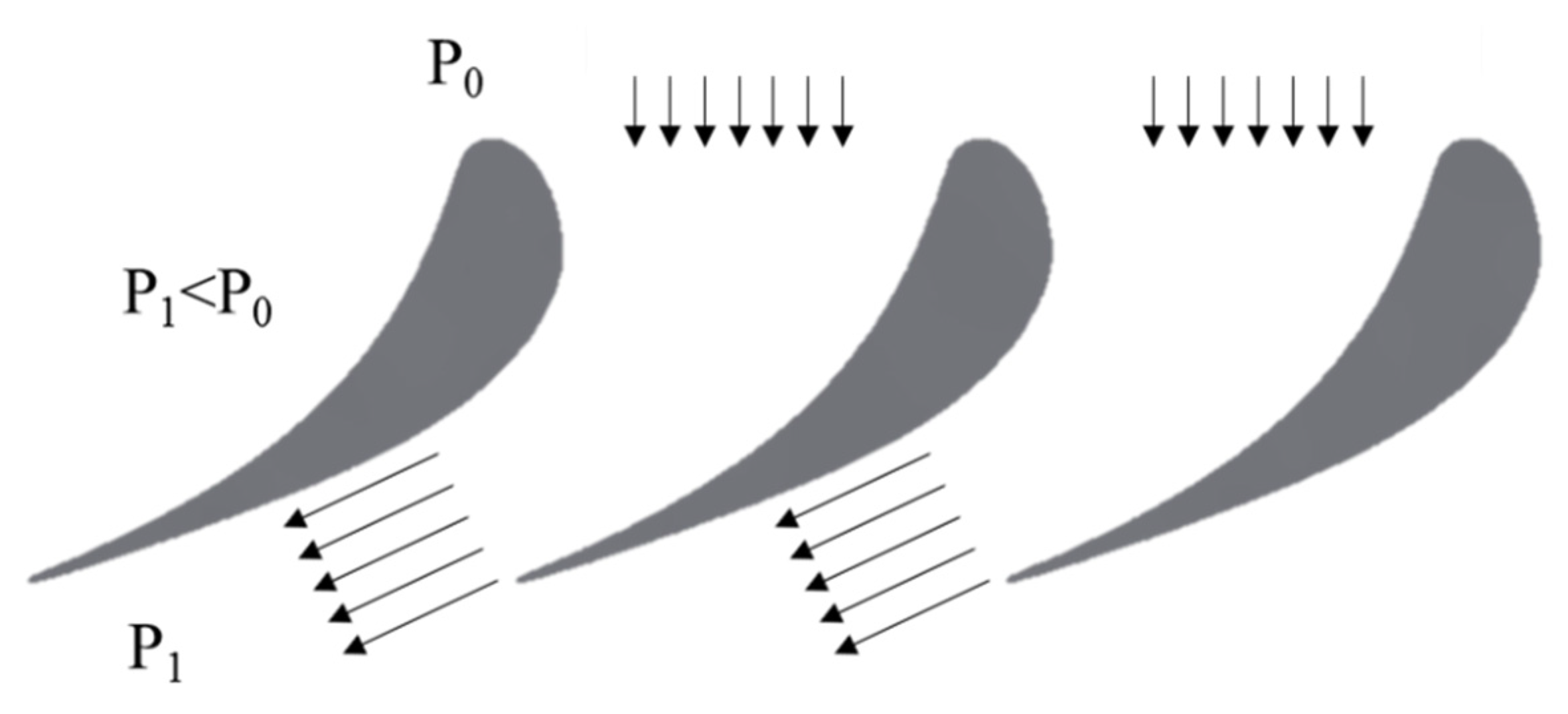
Figure 2.
(a) Geometric characteristics of the turbine blade profiles under study; (b) boundary conditions in preprocessor of the model of the flow volume in a blade channel.
Figure 2.
(a) Geometric characteristics of the turbine blade profiles under study; (b) boundary conditions in preprocessor of the model of the flow volume in a blade channel.
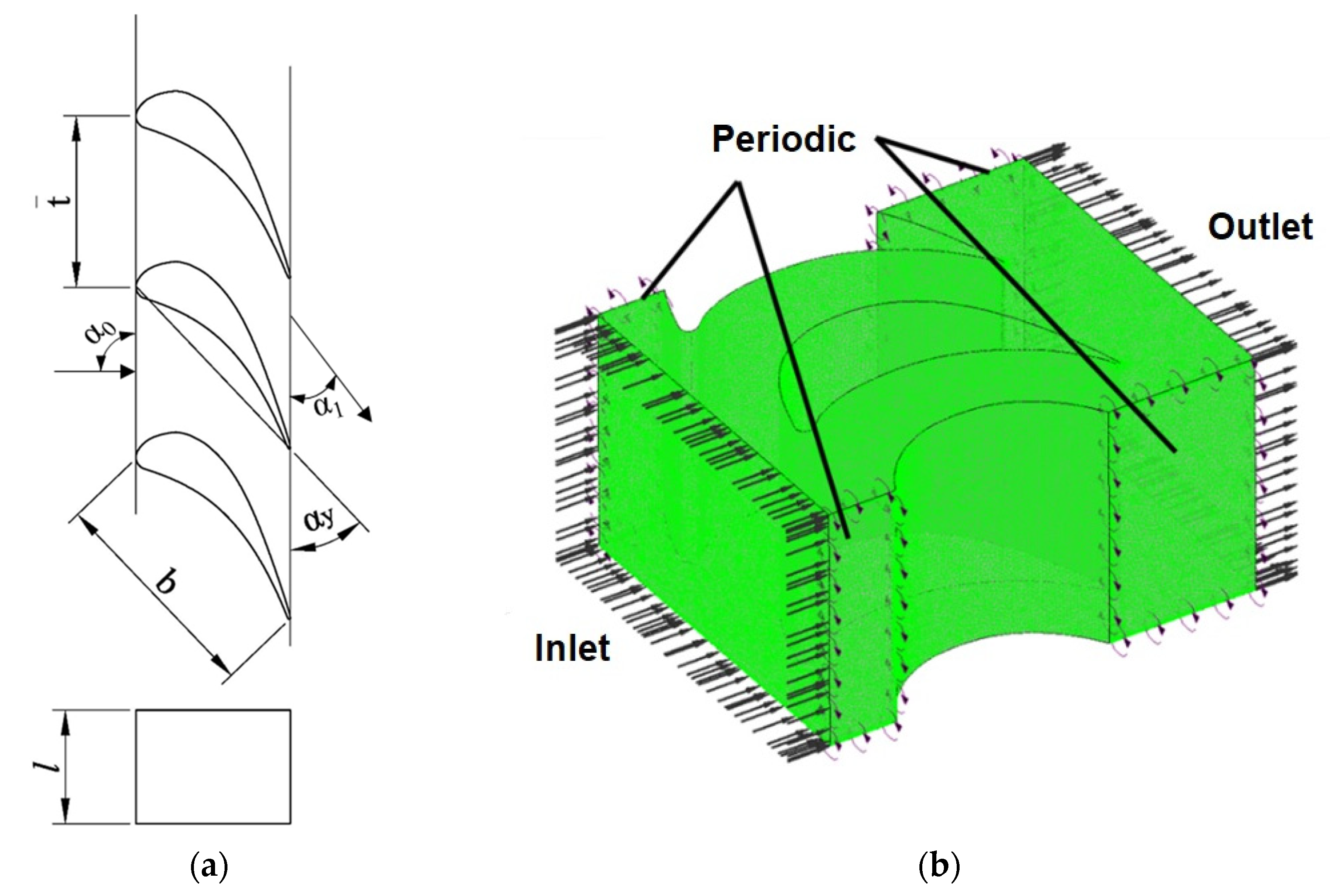
Figure 3.
Computational grid of the flow volume in a blade channel.

Figure 4.
Graph of the error dependence on the Reynolds numbers in a blade channel formed by the C-90-22 A nozzle profile with b/l = 2 obtained using the SST turbulence model.
Figure 4.
Graph of the error dependence on the Reynolds numbers in a blade channel formed by the C-90-22 A nozzle profile with b/l = 2 obtained using the SST turbulence model.
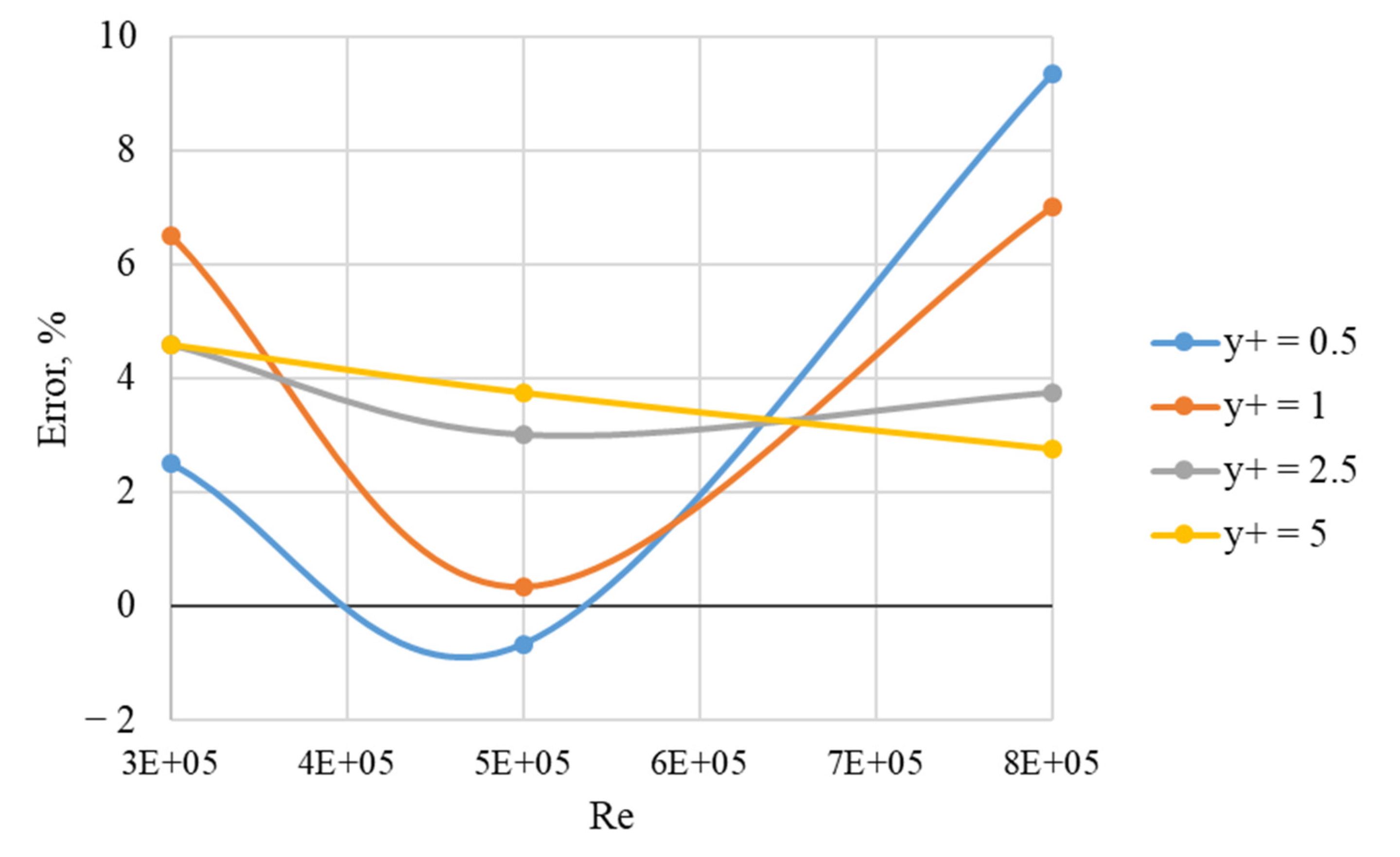
Figure 5.
Graph of the error dependence on the Reynolds numbers in a blade channel formed by nozzle profile C-90-22 A with b/l = 1 obtained using the SST turbulence model.
Figure 5.
Graph of the error dependence on the Reynolds numbers in a blade channel formed by nozzle profile C-90-22 A with b/l = 1 obtained using the SST turbulence model.

Figure 6.
Graph of the error dependence on the Reynolds number in a blade channel formed by nozzle profile C-90-22 A with b/l = 2 obtained using the k − ω turbulence model.
Figure 6.
Graph of the error dependence on the Reynolds number in a blade channel formed by nozzle profile C-90-22 A with b/l = 2 obtained using the k − ω turbulence model.

Figure 7.
Graph of the error dependence on Reynolds numbers in a blade channel formed by nozzle profile C-90-22 A with b/l = 1 obtained using the k − ω turbulence model.
Figure 7.
Graph of the error dependence on Reynolds numbers in a blade channel formed by nozzle profile C-90-22 A with b/l = 1 obtained using the k − ω turbulence model.

Figure 8.
Graph of the error dependence on convergence order: (a) when changing of y+ with constant Re, b/l = 2; (b) when changing Re with constant y+, b/l = 1.
Figure 8.
Graph of the error dependence on convergence order: (a) when changing of y+ with constant Re, b/l = 2; (b) when changing Re with constant y+, b/l = 1.


Table 1.
Geometrical and mode-related parameters of the models under study.
| Parameter | Value |
|---|---|
| b, mm | 45.00 |
| l, mm | 45.00 to 90.00 |
| α0, ° | 90 |
| α1, ° | 22 |
| β1, ° | – |
| β2, ° | – |
| b/l | 1 to 2 |
| 0.75 | |
| αy, ° | 45.7 |
| M | 0.3 to 0.8 |
| Re | 300,000 to 800,000 |
| Maximum linear size of a global element (cell), mm | 1 to 2 |
| Height of the first cell of the prismatic layer, µm | 1.25 to 3.12 |
| Number of prismatic layers | 15 |
| Growth factor of prismatic layers | 1.33 to 1.41 |
| Total height of prismatic layers, mm | 1.0 to 1.1 |
| y+ | 1 to 5 |
| Grid refinement area | trailing edge |
| Maximum linear size of a global element (cell) in the grid refinement area, mm | 0.1 |
| Total number of elements in the computational grid, million | 2.13 to 4.14 |
Table 2.
Boundary conditions for simulating fluid dynamics processes occurring in blade channel.
| Parameter | Value |
|---|---|
| Working fluid | Air IG |
| Working medium flow rate, g/s | 68 to 716 |
| Flow angle upstream of the model, ° | 90 |
| Working medium temperature upstream of the model, °C | 20 |
| Static pressure downstream of the model under study, atm | 1 |
Publisher’s Note: MDPI stays neutral with regard to jurisdictional claims in published maps and institutional affiliations. |
© 2022 by the authors. Licensee MDPI, Basel, Switzerland. This article is an open access article distributed under the terms and conditions of the Creative Commons Attribution (CC BY) license (https://creativecommons.org/licenses/by/4.0/).
Share and Cite
MDPI and ACS Style
Osipov, S.; Shcherbatov, I.; Vegera, A.; Bryzgunov, P.; Makhmutov, B. Computer Flow Simulation and Verification for Turbine Blade Channel Formed by the C-90-22 A Profile. Inventions 2022, 7, 68. https://doi.org/10.3390/inventions7030068
AMA Style
Osipov S, Shcherbatov I, Vegera A, Bryzgunov P, Makhmutov B. Computer Flow Simulation and Verification for Turbine Blade Channel Formed by the C-90-22 A Profile. Inventions. 2022; 7(3):68. https://doi.org/10.3390/inventions7030068
Chicago/Turabian StyleOsipov, Sergey, Ivan Shcherbatov, Andrey Vegera, Pavel Bryzgunov, and Bulat Makhmutov. 2022. "Computer Flow Simulation and Verification for Turbine Blade Channel Formed by the C-90-22 A Profile" Inventions 7, no. 3: 68. https://doi.org/10.3390/inventions7030068