
Extruder Machine Gear Fault Detection Using Autoencoder LSTM via Sensor Fusion Approach


Department of Mechanical Engineering (Department of Aeronautics, Mechanical and Electronic Convergence Engineering), Kumoh National Institute of Technology, 61 Daehak-ro, Gumi-si 39177, Gyeonsang-buk-do, Republic of Korea
*
Author to whom correspondence should be addressed.
Inventions 2023, 8(6), 140; https://doi.org/10.3390/inventions8060140
Submission received: 29 September 2023
/
Revised: 29 October 2023
/
Accepted: 31 October 2023
/
Published: 2 November 2023
(This article belongs to the Special Issue From Sensing Technology towards Digital Twin in Applications)
Abstract
:In industrial settings, gears play a crucial role by assisting various machinery functions such as speed control, torque manipulation, and altering motion direction. The malfunction or failure of these gear components can have serious repercussions, resulting in production halts and financial losses. To address this need, research efforts have focused on early defect detection in gears in order to reduce the impact of possible failures. This study focused on analyzing vibration and thermal datasets from two extruder machine gearboxes using an autoencoder Long Short-Term Memory (AE-LSTM) model, to ensure that all important characteristics of the system are utilized. Fast independent component analysis (FastICA) is employed to fuse the data signals from both sensors while retaining their characteristics. The major goal is to implement an outlier detection approach to detect and classify defects. The results of this study highlighted the extraordinary performance of the AE-LSTM model, which achieved an impressive accuracy rate of 94.42% in recognizing malfunctioning gearboxes within the extruder machine system. The study used robust global metric evaluation techniques, such as accuracy, F1-score, and confusion metrics, to thoroughly evaluate the model’s dependability and efficiency. LSTM was additionally employed for anomaly detection to further emphasize the adaptability and interoperability of the methodology. This modification yielded a remarkable accuracy of 89.67%, offering additional validation of the model’s reliability and competence.
1. Introduction
The recent industrial revolution has had a significant impact on the production and manufacturing sectors, with more advancements on the way. Many industry revolutions have come and gone in the world of research and academia with the aim of increasing and modifying the relationship between man and machine, which is accomplished through the intelligent integration of the Internet of Things (IoT) and cyber–physical systems [1,2,3]. The current phase of the industrial revolution, Industry 4.0, has made technology available in a way that allows for seamless and smart decision making, which has generally improved efficiency and revenue in these sectors. One of the most important aspects of Industry 4.0 is its application in the prognostics and health management (PHM) of equipment, which entails detecting anomalies as well as predicting when these systems may fail, thereby providing a healthy and conducive environment for production. Most of the time, this is accomplished through the use of various types of sensors to collect rich data from these machines in collaboration with a machine learning algorithm that sequentially trains to understand the nature of the data and then aids in the detection and early prediction of any future fault occurrences using advanced technology [4,5]. Most of the means associated with useful data collection from machines for adequate health monitoring include, but not limited to, vibration sensors, acoustic emission sensors, thermal sensors, current sensors, and so on. The selection of the appropriate sensor to be used on equipment is solely dependent on the nature of the machine, the type of environment, and the researcher’s expertise. The next industrial revolution, Industry 5.0, is intended and projected to be more sophisticated and advanced in the sense that machines not only assist humans but also collaborate with humans in solving technical problems [6].
The plastic/fabric extruder machine is a critical piece of equipment in the plastic manufacturing industry. Its working principle entails collecting plastic raw materials through its hopper, which is then directed to the extruder screw, whose pressure and rotation are provided by the gear and an electric motor combined with the machine’s heater pad to melt the plastic raw materials as well as transport them to the chamber where the molten plastic would be used to achieve whatever purpose it has been assigned in terms of shape. Nonetheless, the machine’s effectiveness is dependent on the flawless performance of its components. Among these, the extruder screw stands out as a critical component of the plastic extruder machine. As a result, ensuring the continuing functionality of this specific component becomes critical. The reason for this monitoring is that any fault in the extruder screw could have serious consequences for the manufacturing process. The induction motor provides the required rotary power and torque, while the gear as shown in Figure 1 reduces the rotational speeds of the extruder screw, resulting in more torque for crushing and transporting raw materials. There has been a lot of research on fault diagnostics and prediction in induction motors [7,8,9], but the focus of this research is on the gearbox, whose failure would be catastrophic in the sense that the operational movement and rotation of the extruder screw, which has been designed to provide the required amount of torque and pressure for the manufacturing process, would be greatly affected. In our study, the gear component of the plastic extruder gearbox is made up of helical gears, which are known for their high contact ratio and thus provide high torque [10].
While vibrations are frequently anticipated to come from the running gears, vibration sensors are among the most popular sensors for condition-based gearbox monitoring. Unfortunately, unlike spur gears, helical gears are known to produce less noisy and non-stationary vibration signals due to their contact ratio difference; however, noise and non-stationary signal generation are common with gears, which are regarded as challenges for most signal processing methods [11,12]. Nonetheless, scientists have devised solutions to this problem, such as fusing vibration data with other sensor data like sound and thermal data, or denoising and decomposing vibration data signals to extract the important spectral properties of the signal [13,14]. Most known classes of helical gear failures often cause unusual friction between the meshing and/or mating gear components, which generates heat, making thermal data useful for fault analysis in helical gearbox fault detection and isolation (FDI) [15].
Generally, time-frequency signal transformations are preferred, especially in helical gearbox vibration signals because they present the signal in such a way that useful information can be easily extracted or detected in a signal, which aids in fault diagnosis. Nonetheless, the AE-LSTM is well recognized for its capacity to identify faults or function in multivariate time-domain signals. As a result, the AE-LSTM is an excellent tool for processing and training a fusion of thermal and vibration datasets for proper FDI [16,17]. Machine learning (ML) algorithms have long been used by scientists owing to their efficiency and adaptability to small datasets, as well as their high diagnostic and prognostic accuracy, low computational cost, and ease of implementation. However, due to some of its well-known issues, including their propensity for over-fitting, poor performance with complex datasets, and high parameter dependence, Artificial Neural Network (ANN)-based algorithms, such as Feed-forward neural networks (FNNNs), Long Short-Term Memories (LSTMs), Deep neural networks (DNNs), Deep belief networks (DBNs), Recurrent neural networks (RNNs), Convolutional neural networks (CNNs), etc., have presented the ideal sophisticated diagnostic and prognostic tool, despite their unique challenges such as high computational cost and interpretability issues; however, their uniqueness and robustness in PHM is no match for traditional ML algorithms. Furthermore, the ANNs mentioned which are often referred to as the second generation of ANNs, are recognized for their high computational costs, stemming from their layered architecture which includes hidden layers. Despite this, their efficiency has endured and remains prevalent in recent academic research. Nevertheless, there has been a notable shift in academia toward the adoption of the third generation of ANNs, known as Spiking Neural Networks (SNNs), which offer potential alternatives. SNNs are regarded as the third generation of ANNs, which are known to perform better and also display a lesser computational cost than the second generation ANNs [18,19]. The authors of [19] presented a comparative analysis between artificial and spiking neural networks in machine fault detection tasks using reservoir computing (RC) technology. RC, which acts as an optimizer, employs untrained internal layers (the reservoir), influenced by input and the environment, while optimizing connection weights solely at the output layer. This immutability streamlines learning, a significant advantage that has been shown in various academic journals [18,19,20]. In their research, ball bearing fault detection using an induction motor phase current signal show that second-generation ANN reservoir architecture is significantly inferior both in accuracy and computation cost. Nonetheless, our study utilized second-generation ANNs within the scope of our expertise, as the efficient implementation of SNNs demands a higher level of skill acquisition.
Gearboxes play a critical role in industrial domains, particularly in contexts involving torque transfer, speed reduction, and motion dynamics modification, among other activities. As a result, the consequences of gearbox failure resonate far and wide. Any failure, regardless of the underlying reason, has the potential to produce unneeded downtime. The resulting operational stop reduces productivity by hindering industrial processes. Furthermore, the resulting output shortage directly leads to a revenue loss. The interdependence of gearbox functionality and industrial processes emphasizes the importance of preventive maintenance and constant monitoring to avoid potential failures. Mitigating the danger of gearbox failure by such methods not only ensures operational continuity but also protects against the tangible economic ramifications of stopped output and financial losses. As a result, grasping the basic properties of faults is a fundamental prerequisite in the pursuit of effective fault mitigation within mechanical systems. This includes determining their frequency, patterns of occurrence, and severity. This early understanding serves as the foundation for developing meticulous tactics for correcting these flaws as effectively as possible. A significant insight comes when considering the gearbox in a plastic extruder machine, where the prevalent failures are directly linked with gear-related concerns. While helical gears are more resistant to failure than spur gears, failure is an unavoidable possibility.
Numerous failures have been extensively researched and documented in the academic world. These include broken teeth, fissures, the occurrence of pitting corrosion, uniform wear, axis alignment inconsistencies, fatigue-induced difficulties, instances of impact induced fractures, and the likes. Surprisingly, amid this spectrum of failures, those linked to fatigue phenomena have emerged as the most common [21,22,23,24]. Notably, the prevalence of fatigue-related failures broadens its impact, serving as a critical precursor for additional severe and catastrophic defects within the system [24]. Tooth bending fatigue and surface contact fatigue are the two main types of fatigue failure, which are typically linked to issues with gear assembly, misalignment, unintentional stress concentration, and unsuitable material choice or heat treatment [24,25]. Gear tooth wear is a similarly common form of failure to fatigue in terms of prominence. This failure mechanism involves the loss of gear material and frequently results from many triggers that include mechanical, electrical, and chemical effects [25]. Fundamentally speaking, abrasive and adhesive wear are distinguished modes of tooth wear failures. Adhesive wear is characterized by material transfer between teeth, which leads to propensities for ripping and welding, as opposed to abrasive wear, which includes material removal as a result of inter-tooth contact [25,26]. Scuffing is a key failure mode that is frequently ignored in gear analysis. This occurrence results from sliding motions interacting with lubricated contacts, which generate high temperatures. These elevated temperatures can consequently cause the surface film that coats the gears to deteriorate, leading to deformations and eventually the melting of the relatively softer gear components [25,26,27].
The accuracy of relying exclusively on vibration signals for precise defect identification may be compromised by the elevated levels of noise and temperature that frequently accompany malfunctioning gear conditions. As a result, many researchers have implemented techniques to improve diagnostic precision. These methods often entail either applying denoising techniques to separate important signals from the noise-contaminated vibration data originating from gear components or combining vibration signals with other sensor outputs to create comprehensive diagnostic models. The incorporation of vibration and acoustic sensor data helped the development of a thorough diagnostic model, as demonstrated by the researchers in [28]. Their method involved the independent extraction of statistical features from each sensor. Relevant attributes were identified using a cutting-edge feature selection method. In the end, a comprehensive diagnostic model specifically designed to solve chipped gear defects was developed by synergistically combining the chosen features from both sensors. In a different study [29], the author skillfully combined current and vibration sensors operating over a range of frequencies to create a condition-based monitoring framework for spotting gear wear issues. The study’s conclusions emphasized not only the attainment of desired results but also a calculated approach for reducing the computing demands generally connected with data fusion. This was accomplished by carefully assessing the dataset to only include the most pertinent qualities, and then strategically incorporating statistical and heuristic feature engineering techniques.
Additionally, Zhang Y. and Baxter K. proposed a cross-domain fault diagnostic framework by synergistically combining vibration and torque information from a gearbox in a different exploration [30]. Their ground-breaking approach addressed a common issue that arises when utilizing different statistics from diverse sensors. To counteract this, they used a fusion strategy in which the various sensor datasets were combined into a single 1-D sample array. Then, as a crucial element of their cross-domain fault diagnostic approach, a CNN-based classifier was used. This innovative method made it possible to integrate several sensor outputs, improving the system’s capacity for diagnostics. Several researchers have made considerable advances in refining sensor fusion approaches, as demonstrated by the approach used in this study [31]. To build a diagnostic model, the author used a trio of sensors—a vibration accelerometer, a microphone, and sound emission sensors—across a variety of operational circumstances. Their process entailed extracting wavelet features from each sensor’s data stream, followed by identifying relevant features. This technique resulted in a powerful model that validated their intended aim. A similar three-sensor fusion technique was discovered in another study involving the prediction of the remaining usable life (RUL) of a hydraulic gear pump in the presence of variable pollution levels [32]. The researchers used a Kalman filter-based linear model to smoothly fuse fault features from three distinct sensor data streams—vibration, flow rate, and pressure signals—in this case. These fused properties were then used as an input for a Bidirectional Long Short-Term Memory (BI-LSTM) network, resulting in the creation of a strong RUL architecture.
Due to the inherent characteristics and different origins of sensor data commonly used in sensor fusion, these datasets often contain intrusive background noise, lack stable patterns across time, and depart from a normal Gaussian distribution. As described in this specific research study [33,34], these variables collectively restrict the extraction of important information from the data. Consequently, it is necessary to use supplementary signal processing techniques to present these datasets in a way that allows for effective information extraction. In the context of our investigation, the vibration datasets acquired from machinery necessitate undergoing a denoising process. This procedure is critical for extracting relevant information from vibration data. The effectiveness of this process is dependent on the robustness of the signal-processing algorithms used and the expertise of the analyst. Numerous methods for denoising and decomposing signals have been introduced, including discrete wavelet transform (DWT), Bayesian filter-based methods, and empirical mode decomposition, the latter of which is based on the Hilbert Huang transform (HHT) [35,36]. Among these techniques, discrete wavelet transform and Bayesian-filter-based algorithms are well-known for their effectiveness and robustness. However, when it comes to performance, empirical evidence has shown that discrete wavelet transform is a better option for both signal denoising and decomposition tasks [36]. This insight acted as a catalyst for its preferential use in our ongoing inquiry.
One of the primary goals of this research is to properly combine vibration sensor data with thermal sensor data to build a reliable PHM scheme. To achieve this integration, appropriate fusion techniques must be used to develop strong health indicators (HIs) for an efficient diagnostic model [37,38,39]. It is critical to note that, while the requirement for a fusion algorithm is undeniable, the technique to be used is significantly dependent on the specific challenge at hand. Local Linear Embedding (LLE), for example, can be sensitive to the choice of nearest neighbors, whereas Principal Component Analysis (PCA) may encounter difficulties when dealing with datasets having a normal distribution. Independent Component Analysis (ICA), on the other hand, is dependable when dealing with non-Gaussian input distributions, particularly when these inputs display statistical independence, as demonstrated in previous studies [40,41]. In a related study [40], the authors conducted a thorough comparison of Independent Component Analysis (ICA) and Autoencoder (AE) approaches. The goal of this study was to synchronize data collection from numerous IJTAG-compatible Embedded Instruments (EIs) and build a machine learning-based system-level model for forecasting the end of life (EOL) in safety-critical systems that use multiple on-chip embedded instruments. According to the findings of the study, the ICA and EI fusion strategy excelled in capturing latent variables for model training, hence improving the EOL prognostic power. In addition, J. Weidong introduced the FastICA compound neural network, an original ICA-based network that makes use of feature extraction from multi-channel vibration measurements [42]. This method shows how ICA has the potential to be used as a strong feature extraction tool for challenging sensor data fusion problems.
As a result, the techniques outlined across the spectrum of reviewed research highlight a common theme: the inherent limits of relying simply on vibration signals for diagnosing gear-related difficulties. This collaborative knowledge acts as a catalyst, propelling us to incorporate a unique methodology into our model. Our method combines vibration and thermal sensor data from a plastic extruder machine’s gearbox. While it has been recognized that malfunctioning gearboxes frequently generate heat due to irregular gear meshing, little study has been conducted to harness thermal signals for comprehensive defect investigation which most recorded studies often focus on thermal imagining rather than thermal data signals. This undertaking is a unique step, resulting from the inspiration obtained from the combination of earlier study findings. Therefore, with all these findings in view, the contributions of this sensor fusion plastic extruder gearbox outlier detection fault-based model are highlighted as follows:
- A DWT for enhanced vibration signal analysis in plastic extruder gearbox fault diagnosis: By incorporating a DWT strategy, the aim is to extract invaluable insights from the vibration signals entrenched in noise. This technique seeks to bolster the efficacy of diagnosing faults within the plastic extruder gearboxes.
- An effective statistical time-frequency domain feature extraction and correlation filter-based selection technique: A method for feature extraction is presented in our investigation, which is particularly effective in the time-frequency domain. Furthermore, a feature selection process based on correlation filters, a technique commonly utilized in feature engineering, is incorporated. This process aims to enhance significant and crucial characteristics, thereby improving the overall performance of the model.
- A multi-sensor fusion using the FastICA technique: Our strategy includes a multi-sensor fusion paradigm aided by the (FastICA) technique. The proposed technique harmoniously blends selected information from multiple separate sensor datasets. This fusion not only condenses data to a single-dimensional array but also preserves the unique characteristics of each source.
- An AE-LSTM outlier detection using a fused multi-sensor dataset approach: We achieved an outlier detection by leveraging an AE-LSTM, which is enabled by a fusion of multi-sensor data techniques. This comprehensive methodology results in a strong framework ready for defect detection in the context of a plastic extruder gearbox.
- A proposed framework validation and proposed global evaluation metrics: A set of global evaluation indicators are provided to validate our suggested approach. These evaluations highlight the framework’s efficiency and efficacy, demonstrating its ability to manage the complexities of defect detection within plastic extruder gears.
2. Materials and Methods
The choice of materials and methodologies adopted in the event of a study goes a long way in determining the robustness and efficiency of the output. This section explains the necessary materials and the essential principles underlying the key elements that constitute the foundation of our research. These include DWT for denoising and signal decomposition; FastICA for feature dimension reduction; an overview of AE-LSTM; and the proposed outlier detection model which constitutes the materials, processes, sequences, and the application of the process model for fault detection.
2.1. DWT for Denoising/Decomposition Overview
The wavelet transform is a signal analysis mathematical tool. Through a succession of wavelets, it decomposes signals into multiple frequency components at different scales, capturing both time and frequency information. This enables localized signal feature analysis, which is important for tasks like denoising, compression, and feature extraction. These series are produced by orthogonal functions and indicate a square-integrable function, whether real or complex-valued [33,34]. Just like DFT and STFT which are often used in situations where the fast Fourier transform (FFT) falls short in performance, the wavelet transform as highlighted earlier is a time-frequency signal process tool that is a unique and efficient tool that can present a signal in an orthogonal or non-orthogonal format using basic a function known as a wavelet [34,43]. Generally, the essential difference is in the decomposition approach: the Fourier transform (FT) divides a signal into its sinusoidal components, whereas the wavelet transform employs localized functions (wavelets) that exist in both real and fourier space. Because of this localization in both domains, the wavelet transform can provide more intuitive and interpretable information about a signal. Wavelet transform, as opposed to FT which focuses on the frequency of a signal in most cases, incorporates both time and frequency characteristics, allowing for a more dense study of signals with localized features.
As a mathematical tool, the general equation of a wavelet transform is presented thus in Equation (1):
a and represent the scale parameter and the normalization factor for energy conservation, which regulates the dilation of the wavelet function of the transform, b represents the translation parameter across the time axis, represents the mother wavelet, and represents the complex conjugate of the presented mother wavelet.
In academia, the two most prevalent wavelet transforms are discrete wavelet transform and continuous wavelet transform (CWT). Their main distinction is the function used in their computation. For example, in the creation of a DWT, an orthogonal wavelet is frequently used, whereas CWT adapts a non-orthogonal wavelet. Because of the nature of the signal retrieved from the extruder gearbox, which is embedded with noise; hence, the study focused on DWT. DWT is well known for its usage in signal denoising and decomposition into distinct levels. The Discrete Wavelet Transform (DWT) transforms a signal into approximation and detail coefficients at different scales. The approximation coefficients indicate the low-frequency content of the signal, whereas the detail coefficients represent high-frequency features. This iterative technique gives a multiscale examination of the signal, allowing for efficient representation, compression, and signal processing. The coefficients can be used for signal reconstruction and additional analysis.
The general equation for obtaining the wavelet transform is shown in Equation (2).
k represents the scale or level of decomposition, m represents the translation or position in each decomposed level, is the discrete-time signal being transformed, [n] represents the discrete wavelet function.
The performance of a wavelet is solely based on the wavelet function (mother wavelet). Therefore, it is important to note that the wavelet function’s specific form differs depending on the wavelet family (e.g., Haar, Daubechies, Morlet, etc.). The aforementioned formulas represent the wavelet transform’s conceptual structure, while the actual computation includes evaluating the integral or sum over the proper ranges.
2.2. FastICA for Dimension Reduction
Primarily, ICA was created to solve the problem of blind source separation in image and audio processing. Its major goal was to extract from observed signals a set of statistically independent components. FastICA was created in response to the potential of ICA for dimensionality reduction, specifically for feature fusion [40]. In many circumstances, the mutual information among numerous aspects is buried by high-order statistical characteristics, and FastICA is successful at minimizing high-order correlations while maintaining mutual independence among these features. FastICA is thus a useful tool for reducing dimensionality by merging characteristics while keeping their independence [40,41,44].
FastICA is a signal decomposition algorithm that divides observed signals into statistically independent components. It assumes the signals are a mixture of unknown sources and attempts to estimate the original sources by maximizing their independence. The procedure begins by centering the signals and then whitening them to remove correlations and equalize variances. To quantify the divergence from gaussianity in the altered signals, a measure of non-gaussianity, such as negentropy, is used [43,44]. FastICA maximizes this metric iteratively by updating the weights of linear combinations of the observed signals. After obtaining the independent components, dimensionality reduction can be accomplished by picking a selection of components that capture the most relevant information or contribute the most to the original signals. The dimensionality of the data is efficiently decreased by removing less relevant components. The reconstructed signals can then be obtained by projecting the independent components back. For our study, FastICA is presented due to its prowess in fault detection scenarios the more discriminant the data the better it is for the training model to easily adapt and classify and/or detect the presence of abnormality in a set of data.
2.3. Correlation Coefficients
Correlation coefficients are statistical measurements that assess the degree and direction of a relationship between two variables. The Pearson correlation coefficient, Spearman rank-order correlation coefficient, and Kendall rank correlation coefficient are three regularly used correlation measurements. The Pearson correlation coefficient evaluates the linear relationship between variables. It is calculated by dividing the covariance of the variables by the product of their standard deviations. Pearson correlation coefficients vary from −1 to 1. A value of −1 indicates a strong negative linear association, 0 shows no linear relationship, and 1 suggests a strong positive linear relationship. It is commonly symbolized by the symbol (rho). The Spearman rank-order correlation coefficient, on the other hand, is a non-parametric statistic that assesses the strength of a monotonic relationship between variables. It is based on the data ranks rather than the actual data values. Its range, like the Pearson correlation coefficient, is from −1 to 1, with −1 indicating a strong negative monotonic association, 0 suggesting no monotonic link, and 1 indicating a strong positive monotonic relationship. The Kendall rank correlation coefficient is another non-parametric statistic that assesses the strength of the monotonic association between variables. It takes into account the number of concordant and discordant pairs in the data.
Thus, in our study and the majority of studies involving linear variables, the Pearson correlation coefficient is frequently selected above alternative correlation coefficients. The other two types, however, operate more effectively than the Pearson correlation in situations involving non-linear variables. The general mathematical expression for Pearson correlation, Spearman correlation, and Kendall rank correlation are represented in Equations (3)–(5). The correlation coefficient has generally been used successfully in academia for feature reduction, selection, diagnostics, prognosis, and other tasks. The Pearson coefficient was used in this study to extract meaningful and discriminant features, which is essential for effective problem diagnosis and fault detection [7,8,43,45].
represents the Pearson correlation coefficient, n represents the number of data points, x and y represents the variables being compared, represents the Spearman correlation coefficient, d represents the difference between the ranks of corresponding data points of the two variables, represents the Kendall rank correlation coefficient, P and Q represent a concordant pair (pairs of data points for which the ranks of both variables follow the same order) and discordant pairs (pairs of data points for which the ranks of the two variables follow opposite orders), respectively, and and represent the variables being compared.
2.4. Autoencoder
AEs are a form of artificial neural network that is used to learn input data representations. They are made up of three basic parts: an encoder, a bottleneck layer, and a decoder. In the bottleneck layer, the encoder maps the input data to a compressed representation. The bottleneck layer acts as a bottleneck for information flow, lowering the input’s dimensionality. The latent space representation is the learned representation in the bottleneck layer. The decoder attempts to recover the original input data using the latent space representation. The AE’s purpose is to reduce the reconstruction error, which is the difference between the input data and the reconstructed output.
By defining the problem as a supervised learning task, AEs can be trained with the aid of unlabeled data. The goal is to produce an output that closely resembles the original input. This is accomplished by reducing the reconstruction error, for instance (x,), where x is the initial input sequence and is the resultant reconstruction sequence. The AE learns to extract relevant features from input data and build a compressed representation in the latent space by iteratively modifying the network’s parameters. As a result, AEs can be used for tasks like dimensionality reduction, data denoising, and anomaly detection [3,46,47,48].
2.5. Long Short-Term Memory (LSTM)
LSTM networks were created to get around regular RNNs’ limitations when processing lengthy sequences. To capture and hold long-term dependencies in sequential data, they contain memory cells and gating mechanisms. A memory cell used by LSTMs serves as a conveyor belt for information as it moves through the sequence. Long-term memories are stored in the cell state, and what should be discarded is decided by the forget gate. The output gate regulates the output depending on the cell state, whereas the input gate controls fresh information that is added to the cell state. Because they have the capacity to learn and spread pertinent information over lengthy sequences, LSTMs excel at jobs involving sequential data.
The mathematical expression for the LSTM architectural structure is defined with the following Equations (6)–(12):
i, f, O represents the input, forget, and output gates, describes the current input to the LSTM architectural structure, , , , represents the cell state, previous cell state, the hidden cell state, and the previous hidden cell state, respectively, and , W, b represents the sigmoid function, weight and bias of each gate [49,50,51,52].
For a more insightful explanation of the structure of the LSTM; LSTMs employ gates that permit selective information memory retaining and forgetting, allowing them to update the cell state based on the current input and past state. The input gate applies an activation function to the input and previous hidden state (such as sigmoid, ReLU, or softmax), yielding values between 0 and 1. These values are then multiplied element by element-wise with the input, with their importance scaled accordingly. The forget gate generates values between 0 and 1 by applying a sigmoid function to the input and prior concealed state. These values are then multiplied element by element with the prior cell state, with the previous values scaled according to their importance. Values between 0 and 1 are produced by the output gate after applying a sigmoid function to the input and prior concealed state. The output of applying a hyperbolic tangent function to the current cell state is then multiplied element-wise by these values to produce the LSTM’s final output. A vector of values that is updated at each time step makes up the cell state of LSTMs. Utilizing the current input, the prior cell state, and the prior concealed state, the cell state is updated. Following that, the hidden state, which is utilized to make predictions, is updated using the revised cell state [53,54,55].
2.6. The Proposed Outlier Detection Model
In the study, an AE-LSTM deep learning approach is employed to create an anomaly detection model. Anomaly detection entails recognizing patterns that differ clearly from the usual pattern in a given dataset. Anormality detection seeks to distinguish uncommon datasets, known as anomaly datasets, from normal datasets. Many strategies have been developed in academia to detect anomalies [3,8,45,56,57], such as statistical methods, machine learning algorithms and data visualization approaches; supervised, semi-supervised, and unsupervised learning approaches; outlier detection; the clustering technique; and so on, are some of the commonly used techniques employed for anomaly detection, where presented models learn the normal patterns or structures from the data without explicitly labeled anomalies. Once trained, the models can detect outliers from learned usual behavior and highlight them as potential abnormalities.
Figure 2 displays the anomaly detection model employed in our study. We employed an outlier detection methodology with the aid of an AE-LSTM deep learning approach. The model consists of five major steps which are summarized below.
- Data acquisition: Both vibration and thermal data were collected in order to construct an appropriate model for monitoring extruder gear performance. The incorporation of several data sources is prompted by the fact that vibration signals obtained from gearboxes are prone to noise contamination, making it difficult to extract valuable insights on their own. A more comprehensive and useful picture can be built by adding additional data, such as temperature measurements. Vibration data are critical for detecting anomalies or inconsistencies in the operation of the gear. However, because of the existence of noise, it is frequently impossible to distinguish important patterns or trends purely from vibration signals. This is when the extra thermal data come into play. By combining vibration and thermal data, it is possible to identify hidden links and correlations between the performance of the gear and the accompanying temperature fluctuations. The use of both vibration and thermal data seeks to improve the accuracy and usability of the model built to monitor the extruder gear. This method allows for a more comprehensive study, allowing for the detection of potential problems such as high friction, overheating, or abnormal operating circumstances. Finally, by combining multiple data sources, a more robust and efficient model may be constructed, providing useful insights for optimizing extruder gear performance, maintenance, and dependability.
- Signal processing and feature extraction: The second key aspect of the model revolves around signal processing, with the aim of extracting valuable information from gearbox vibration data while minimizing the inherent noise. The DWT was used as a method for deconstructing, filtering, and pre-processing the vibration signals to achieve this. The DWT extracted time-frequency statistical information from both the original signal and each vibration signal decomposition level. A full analysis of the vibration data was performed by performing decomposition at various levels, collecting variances across different scales and frequencies. Thermal data, on the other hand, as a time-varying signal, did not go through decomposition. Instead, from the raw temperature data, time statistical features were extracted. The goal of this method was to capture the temporal patterns and trends revealed by temperature readings. The study aims to improve the quality and usability of the information gained by applying the DWT to vibration signal processing and extracting time statistical features from temperature data. This methodology allowed us to identify key trends, correlations, and anomalies in the vibration and temperature data, allowing us to gain a more comprehensive understanding of the extruder gear’s behavior and performance.
- Feature selection: To obtain an effective diagnosis in the setting of anomaly detection, discriminant traits are required. A correlation filter technique was used to guarantee that the features extracted had enough discriminative power. This technique ensures that only features with a correlation percentage of 70% or above are deemed closely connected. By removing characteristics that do not match this correlation threshold, the resulting feature set is tailored to include informative and discriminating features, improving the accuracy and effectiveness of the diagnosis process.
- Signal fusion: The integration of data from numerous sources while keeping their different characteristics is a critical step in our suggested model’s signal data fusion. FastICA was used as the signal-processing method in our study for this reason. FastICA aided us in the merging of data from several sources, allowing us to mix and extract important information while preserving the distinctive qualities of each data source. We accomplished effective signal integration using FastICA, allowing for a thorough analysis that captures the synergistic effects and correlations across the various data sources in our investigation.
- Diagnosis/outlier detection: The entire model’s procedures are built with the goal of detecting faults, specifically through outlier detection. The model’s structure is deliberately constructed to accomplish this aim. As for the AI tool of choice in our investigation, an AE-LSTM was employed. Details concerning the implementation and operation of the AE-LSTM have been discussed earlier in this section. The overarching goal is to use this AI tool to discover issues by finding anomalies in data, allowing for prompt diagnosis and intervention.
2.6.1. Model Hyper-Parameter Function
In the hidden layers of neural networks, activation functions are used to introduce nonlinearity, which is critical for representing complex input. For instance, linear regression models are insufficient for most data representations because they lack nonlinear activation functions. Sigmoid, tanh, and ReLU (Rectified Linear Unit) are examples of common activation functions that are often employed in deep-layer neural networks. In binary classification tasks, the sigmoid function transfers inputs to a range of 0 to 1. However, given big input values, it can saturate, inhibiting learning. The tanh function is similar to the sigmoid function; however, it maps inputs to a range of −1 to 1.
On the other hand, ReLU has grown in popularity as a result of its capacity to improve training efficiency and effectiveness. Positive inputs are kept while negative inputs are set to 0. ReLU can experience the “dying ReLU” problem when neurons stuck in the negative area become inactive, despite its simplicity and computational efficiency. Loss functions, also known as cost functions, estimate how much the actual ground truth departs from the outputs that were projected. Various task kinds are catered for by various loss functions. Cross-entropy loss is appropriate for classification jobs while mean squared error loss is frequently utilized for regression activities. When developing deep learning models, the loss function is minimized by changing the model’s weights and biases. Iterative optimization is used to improve the model’s performance and accuracy. The mathematical equations for some of the regularly employed activation functions , , and are presented in Equations (13)–(15), respectively.
, , represent sigmoid, relu and softmax functions, respectively, x represents the input class which can be any real number.
The success of a model is often determined by the architecture chosen, a decision that is often reliant on the researcher’s knowledge and experience. Table 1 details the Architecture Parameters of the model used in our analysis.
2.6.2. Model Global Performance Evaluation Metrics Overview
It is critical to thoroughly examine the diagnostic skills of various deep learning while taking into account variables like model complexity, computational needs, and parameterization in order to accurately estimate their capabilities. This makes the use of defined criteria for assessing performance and discriminating necessary. These parameters include F1-score, accuracy, sensitivity, precision, and false alarm rate. By using these measurements, we can compare and objectively assess the performance of various models, allowing us to make well-informed decisions based on their individual advantages and disadvantages. Some of the known global evaluation metrics employed in studies are presented thus in Equations (16)–(20).
where and , respectively, are the numbers of accurately classified groups, numbers of inaccurately classified groups, numbers of inaccurately labeled samples that belong to a group that was accurately classified, and the number of inaccurately labeled samples belonging to a group that was inaccurately classified. It is essential to evaluate categorization models in order to judge their effectiveness and dependability. Although metrics like true positives (TP), false positives (FP), true negatives (TN), and false negatives (FN) give a general picture of classification accuracy, it is frequently required to assess the performance of each specific class to get a more complete picture. Take the case of a classifier that completes a five-class issue with an overall accuracy of 95%. This apparently great accuracy may really be the consequence of the model’s ability to categorize three or four of the five classes accurately while misclassifying the other one or two classes. However, in the case of an outlier detection model as in the case of our model, determining these metrics helps assess the model’s performance in accurately identifying outliers while minimizing false positives and false negatives, ensuring effective outlier detection not just for the instance but also when employed in other instances.
This discrepancy underlines the necessity for the confusion matrix, which enables us to assess the diagnostic efficacy of each class in a model. The confusion matrix gives a thorough examination of the predictions made by the classifier/outlier, dividing them into true positives, false positives, true negatives, and false negatives for each class. a model’s performance may be evaluated more carefully by understanding where it performs best or worse by examining its confusion matrix.
In conclusion, while global metrics offer an overall evaluation of classification accuracy, assessing class-specific performance using the confusion matrix is essential to spot any inconsistencies or biases and to make defensible choices about the validity of a classification model.
2.7. Data Collection and Pre-Processing
This section discusses the data acquisition process, sensor placement, signal processing, feature extraction, feature selection, and signal fusion. The data employed in the study were acquired from two independent plastic extruder machines (healthy and faulty machines) in SPONTECH.
SPONTECH is a subsidiary of Toray Inc. (Tokyo, Japan); Toray Co. is Japan’s premier chemical and textile conglomerate, with an unrivaled No. 1 position in carbon fiber, as well as Japan’s leading material giant, producing engineering plastics, IT materials, and chemical fibers in addition to carbon fibers.
Figure 3 depicts the setup of individual sensors on the plastic extruder machine. These sensors are deliberately critically placed to collect crucial information that will be used to generate a dataset with useful characteristics when examined. As previously stated, two plastic extruder machines were used in this study. The first machine as seen in Figure 4a had been running for less than four months, and its data is designated as the healthy dataset.
The second machine, represented in Figure 4b, had been in service for more than two years and had a chipped gear tooth. This machine (with the chipped gear tooth) was used to create the faulty dataset. In the study, evaluation and analysis of the variations between the healthy and faulty situations are achieved by incorporating data from these two machines in order to get insights into the performance and potential concerns of the plastic extruder machines.
Figure 5a,b depicts a visualization of time-domain data gathered from the vibration and thermal sensors respectively in order to have a better understanding of the data collected from both machines. In our investigation, a shear Piezotronics accelerometer model 353B33 with a vibration sensitivity of 99.2 mv/g was employed for our research. To acquire thermal data signals, an RTD PT100 thermal sensor was used to collect gearbox-generated heat temperature variation. This visualization provides a comprehensive perspective of the data collected from various sensors, allowing us to assess and comprehend the nature of the data signals gathered from the plastic extruder machines used in our research.
From observation in Figure 5a, a little distinction can be seen between the vibration data generated from the healthy and faulty gearbox conditions. The healthy data displayed a uniform periodic pattern throughout the whole range of the dataset, occasionally modulated at various intervals. On the other hand, the faulty data visualization shows a non-consistent behavior across the whole data range; the early part displayed a non-constituent data display while the remaining part of the dataset displayed to an extent a uniform visualization of the dataset. However, it is important to note that this visual representation alone might not necessarily indicate the needed discriminative information for ensuring the effectiveness of an anomaly detection model.
Additionally, Figure 5b shows a comparable data visualization of temperature signals for both the healthy and faulty gearbox. On the other hand, it is noticeable that the temperature measurements in the healthy dataset are a little lower than those in the faulty dataset. The difference is normal given that a damaged gearbox will probably produce higher temperatures than a healthy one. These temperature changes can help spot abnormalities in gearbox performance and offer useful insights into possible variances between the two circumstances.
The substantial quantity of noise contained in the vibration signals produced by gearboxes must be addressed in order to efficiently extract or enhance vital information. As a result, a DWT is used to de-noise the signals for both healthy and malfunctioning gearboxes. The visual representation of the decomposition and denoising of the vibration signal received from the gearboxes is shown in Figure 6. By separating the wanted signal components from the noise using this method, the study was able to emphasize and extract the essential data required for additional analysis and diagnostics.
The Discrete Wavelet Transform (DWT) was applied to both the healthy and faulty gearbox signals, as shown in Figure 6a,b, resulting in a four-level decomposition. This decomposition efficiently decreases the effects of noise in the signals, revealing the time-frequency domain properties of the processed signals. As discussed earlier in the previous chapter, the DWT decomposition generates the approximate and detailed coefficients that represent the signal’s low and high frequencies, respectively. In our investigation, our concentration was primarily on approximate coefficient because it offers more detailed information on the gearbox signal’s significant frequencies and features.
2.7.1. Feature Extraction
DWT are signal processing tools that uniquely transform a signal to its time-frequency domain; thus, time-frequency domain features are frequently used to ensure that useful information is successfully extracted from these signal-presenting features that are rich and contain all of the useful details of a given signal. In our investigation, a multi-sensor approach is employed with only the vibration signal being subjected to a DWT; on the other hand, only time-domain statistical features were extracted from the thermal sensor dataset, which is a time-variant data.
In this study, we used sixteen statistical features in the time domain to evaluate temperature data. In addition, we all employed sixteen time-frequency domain features in analyzing the DWT decomposition of the vibration signal as well as the original signal; the sixteen statistical time-frequency features included twelve time-domain features and four frequency-domain features as summarized in Table 2. Our goal was to extract useful information from the signals in order to improve the model’s efficiency.
It is vital to highlight that no precise criteria were adhered to while selecting statistical features. Instead, our choice was based on the popularity of specific characteristics in the area and the authors’ experience.
2.7.2. Feature Selection and Sensor Fusion
To evaluate the adequacy of the extracted features for our model, we conducted a discriminant test using a Pearson correlation-filter-based approach. This method involved assessing the correlation between features and dropping the features with a correlation of 70% or more leaving behind features below the 70% similarity threshold. Figure 7 and Figure 8 show the correlation plot for both the thermal and vibration extracted features in our study, respectively.
Furthermore, the correlation filter-based model selected five features from the thermal data (shown in Figure 9a) and seven features from the vibration data (shown in Figure 9b). This feature selection process efficiently reduced the dataset, retaining only the relevant and most discriminant features necessary for optimal model performance.
To integrate the multi-sensor data in our study, FastICA (fast independent component analysis) was used to combine multi-sensor data in our investigation. This method was used to keep the distinguishing characteristics of each sensor’s separate qualities while blending them together. The FastICA ensures that the fused data keep the distinct properties of each sensor, allowing us to gather and exploit the essential information from all sensors in a cohesive manner.
3. Results and Discussion
3.1. Proposed System Training and Validation
An AE is a neural network that learns to reconstruct input data from a compressed representation known as encoding. On the other hand, LSTM, a recurrent neural network, is frequently employed in language processing and captures long-term dependencies. To take input data, learn a concise representation, and reconstruct the original input, an LSTM can be incorporated into an AE architecture. The reconstruction loss is used to train the AE. Although the number of features has no direct impact on performance, large amounts of input data could make it harder to learn a decent representation. Performance is influenced by the size, reliability, and selection of the hyperparameters.
AE-LSTMs, like other neural networks, can be trained using common approaches such as stochastic gradient descent and back-propagation. The reconstruction loss, which measures the discrepancy between the input and output sequences, is often used to evaluate network performance. The AE-LSTM can learn to decrease this reconstruction loss and provide accurate reconstructions of the input data by refining the model’s parameters using gradient-based optimization approaches. To create a model that could efficiently determine anomaly in a plastic extruder gearbox, an AE-LSTM architecture was employed in our study; where the LSTM captured the long-term dependency of a given data which in this case a fusion of the machine’s vibration and thermal sensor data, while the AE helps in dimension and also for feature learning. The mean squared error (MSE) is a popular loss function used in the training of an AE-LSTM. The MSE quantifies the average squared difference between the expected and true outputs, indicating the goal of accurately reconstructing the input data. The model is trained on labeled training data and its performance is evaluated on a separate validation set during the training phase. The validation loss is computed on the validation set, while the training loss is computed on the training set. It is critical to monitor the trend of these losses, as a considerable difference between them can suggest over-fitting. Over-fitting happens when the model fits the training data too closely, resulting in poor performance on unknown data. In academia lots of methodologies have been presented in mitigating over-fitting in AE-LSTM, these techniques include dropout, early stop, regularization, data augmentation, earlier data fusion, and reducing model complexity [58]. Some of these techniques are consciously implemented in our model setup to enable an efficient model performance that is void of over-fitting. Figure 10 the training and validation loss for the AE-LSTM model employed in our study.
Figure 10 depicts our model’s effective training, adaption, and validation. It clearly shows the discernible difference between validation and training loss. Notably, throughout the early stages of model training, the difference between the training and validation losses shrank significantly, reaching a point of negligible importance around the 22nd epoch. Because of this convergence, model training was halted at that epoch.
3.2. Model’s Outlier Detection Evaluation
The key objective of our model is to create a framework capable of quickly identifying instances of anomalies within a plastic extruder gearbox. As a result, it is critical to evaluate the model’s performance by subjecting it to our faulty collected data. This technique seeks to assess the model’s competency and precision in finding faults using an outlier fault detection methodology included in the model’s architecture. Also, other evaluation metrics are presented to authenticate our model such as precision, F1-score, accuracy, and accuracy to achieve this goal. These metrics prove valuable when an individual possesses the actual labels of input data and seeks to group the signal. The AE-LSTM’s architecture is composed of 7 layers and encompasses 247,937 parameters; the seven layers include an input layer, four encoder LSTM layers, a repeated vector layer, and a time-distributed layer. A comprehensive depiction of the AE-LSTM model is available in Table 1, showcasing the architecture of our model such as a dropout rate set at 0.001, a total of 100 epochs, a batch size of 32, 7 layers, and 2 classes. To further elaborate on the parameters used in the study—batch size refers to the number of training samples at an iterative training instance for each forward and backward iteration. Batch size ranges from 8 to 32, and 64 to 256 or even more for large datasets. In our case, we employed batch size 32 as our datasets underwent lots of pre-processing, feature extraction, and selection which had an effect on the data size. The rest of our parameters were selected based on expertise and performance. After successfully training our model, an outlier detection technique is utilized in predicting the presence of an abnormality in our faulty dataset. Figure 11 depicts the reconstruction error and the threshold, which demonstrate the principle of the outlier detection technique used in our model; reconstruction error is the difference or discrepancy between the input data and the output data of a model, which occurs frequently when the input data is fed through an encoding and decoding process. In the case of anomaly detection, as used in our model, reconstruction error is frequently used to highlight the dissimilarity between input and output data, perhaps indicating if the data is anomalous or faulty. In our situation, the dataset gathered from the healthy extruder gearbox was used as the training dataset for our model, and the dataset collected from the faulty extruder gearbox as the output dataset.
3.3. Model’s Evaluation Metrics Validation
Global metrics are critical in measuring the performance and efficacy of models across entire datasets or any particular problem the model is intended to address in the realms of data analysis, machine learning, and assessment. When looking for a full understanding of how a model performs across numerous classes, categories, or instances, using global evaluation metrics becomes very important. This method allows for a comprehensive assessment of a model’s strengths and shortcomings across all groups and categories.
To evaluate the model performance in our study, global evaluation metrics such as accuracy, F1-Score, Recall, and Precision were used. These metrics provide a comprehensive picture of how well the model performs in various settings. Our findings are summarized in Table 3, which summarizes the conclusions of our inquiry.
To emphasize the importance of model validation, the confusion matrix technique is introduced. This tool was used to determine whether the presented accuracy corresponds to the predicted labels’ class classifications. Figure 12 presents an overview of the confusion matrix technique on our model. The derived confusion matrix shows that the model’s predictions are proportionally consistent with the accuracy metric, reinforcing the model’s reliability.
Model Validation with LSTM
LSTM emerges as a potent strategy for learning long-term dependencies and efficiently representing the relationship between current events and previous events. The LSTM cell was created to address the vanishing-gradient problem that happens with traditional RNNs and results in the inability to learn long-term dependencies. On the other hand, LSTMs are not as efficient as AE-LSTMs in anomaly identification, which might be attributed to the ability of AE-LSTMs train to minimize reconstruction loss. To evaluate the effectiveness and robustness of our model, we used the sample datasets to execute an anomaly detection with LSTM utilizing our model’s systemic approach. Table 4 represents the parameters employed in building the LSTM architecture for training.
The LSTM model, like our proposed model, was trained and validated using healthy datasets from the plastic extruder machine, as shown in Figure 13. We used an early stop mechanism for training the LSTM in anomaly detection, as evidenced by the training epochs, stopping at the sixth epoch out of the twenty initially selected epochs. We observed a considerable reduction in the training error difference from the second epoch while visualizing the data, demonstrating the model’s potential for further application in anomaly detection. The anomaly detection plot for the LSTM model is depicted in Figure 14. The plot displays fault data, predictions, embedded anomalies within the fault dataset, and the fault detection threshold.
When it comes to operational performance preferences, the AE-LSTM and LSTM models differ in their preference for reconstruction error over anomaly prediction error. AE-LSTM models often prefer reconstruction error, whereas LSTM models favor anomaly prediction error, which quantifies the difference between predicted and actual values. When the prediction error exceeds a predetermined threshold, anomalies are detected. In practice, the best appropriate technique is determined by criteria such as data characteristics, the unique situation at hand, and the available expertise. This choice represents a careful analysis of each model’s capabilities and fits with the specific requirements of the given task, providing flexibility in dealing with a variety of scenarios. Table 5 shows the summary of the performance evaluation metrics for the LSTM model.
As demonstrated, when combined with our proposed strategies, LSTM performed commendably. Just as we used a global assessment metric to validate the model, it is critical to subject it to additional validation using the same or a comparable dataset. This stage reinforces the model’s resilience, adaptability, efficiency, and dependability. The validation method not only confirms the model’s competence but also ensures its adaptation to different settings, highlighting its dependability in numerous applications.
4. Discussion
The primary focus of this research was the integration of two independent data signals, namely vibration and heat data. The method used, which combined the Discrete Wavelet Transform (DWT) for signal processing and denoising with Fast Independent Component Analysis (FastICA) for data fusion, has demonstrated notable efficiency. This is evident in the outstanding performances, with the AE-LSTM and LSTM models achieving accuracy rates of 94.42% and 89.67%, respectively, in their respective outlier fault detection tasks. These findings underscore the effectiveness of the proposed methodology. Nonetheless, a pivotal hurdle encountered in the study revolved around data acquisition, which had a substantial impact on the data collection procedure. This highlighted the need to use appropriate data extraction strategies to achieve the goals of our study.
Future studies might include comprehensive assessments of our model’s accuracy and performance against competing models that use alternative feature extraction and selection strategies. Furthermore, there is the possibility for exploration into the introduction of more complex deep learning algorithms to assess the potential for enhanced efficiency while retaining reasonable computational time frames. For example, while our research primarily concentrated on second-generation Artificial Neural Networks (ANNs), there is a chance to delve into the area of third-generation ANNs, particularly Spiking Neural Networks (SNNs). SNNs are well-known for their ability to attain high accuracy while requiring fewer computational costs, making them an intriguing area for further research. These prospective investigations intend to broaden the scope of anomaly detection by pushing past the boundaries of accuracy, efficiency, and computation feasibility. Notably, despite our model’s 94.42% accuracy, there is still room for significantly better performance results. These efforts would contribute to a thorough understanding of fault detection models, helping the improvement and optimization of our proposed system.
5. Conclusions
Machinery breakdowns can have serious consequences, including downtime and financial losses. Our research focused on the gearbox of a plastic extruder machine, which is primarily made up of helical gears. helical gears, despite their lower susceptibility to failure, are not immune to breakdowns, necessitating the implementation of Condition-Based Monitoring (CBM). Our analysis used a multi-sensor approach, including vibration and thermal sensors. Traditional vibration measurement can be hampered due to the tendency of defective gearboxes to generate excessive noise. Our research resulted in a solid framework that included various methodologies such as the Discrete Wavelet Transform (DWT) for vibration signal decomposition, time-frequency statistical feature extraction, correlation filter-based feature selection, the Fast Independent Component Analysis (FastICA) sensor fusion technique, and an outlier fault detection approach.
One of our study’s main goals was to create a model capable of seamlessly merging different sensors while retaining their inherent properties, which aligned with the study’s overall goal. 16 time-domain features were extracted from the temperature data signals and 16 time-frequency features were extracted from vibration signals to achieve our goal. Following that, an efficient procedure is introduced to select five and seven most important features from the thermal and vibration datasets, respectively. Using the Fast Independent Component Analysis (FastICA) approach, these selected features were harmoniously blended into a single-dimensional representation. Pleasantly, our innovative implementation of the AE-LSTM outlier fault detection technique achieved a remarkable prediction performance accuracy of 94.42%, setting an impressive milestone in our research path. In a commitment to ensuring the integrity of our model, we thoroughly scrutinized our outcomes using a variety of global evaluation metrics. Furthermore, we validated our model technique using LSTM, which produced an accuracy of 89.67%, to confirm its compatibility with other AI learning tools. This additional validation demonstrates the effectiveness and dependability of our model and guarantees its flexibility and resilience when combined with other AI learning techniques. This extensive study served to validate and highlight the robustness and dependability of our proposed system. Overall, our study’s multidimensional approach not only addressed sensor fusion but also demonstrated the potential of our model for effective anomaly detection and classification in the context of plastic extruder gearbox systems.
Author Contributions
Conceptualization, J.-H.L. and C.N.O.; methodology, C.N.O.; software, J.-H.L. and C.N.O.; formal analysis, C.N.O.; investigation, J.-H.L. and C.N.O.; resources, J.-H.L., C.N.O. and J.-W.H.; data curation, J.-H.L.; writing—original draft, J.-H.L. and C.N.O.; writing—review and editing, C.N.O.; visualization, J.-H.L. and C.N.O.; supervision, J.-W.H.; project administration, J.-W.H.; funding acquisition, J.-W.H. All authors have read and agreed to the published version of the manuscript.
Funding
This research was supported by the MSIT (Ministry of Science and ICT), Korea, under the Innovative Human Resource Development for Local Intellectualization support program (IITP-2023-2020-0-01612) supervised by the IITP (Institute for Information and communications Technology Planning and Evaluation).
Institutional Review Board Statement
Not applicable.
Informed Consent Statement
Not applicable.
Data Availability Statement
The data presented in this study are available upon request from the corresponding author. The data are not publicly available due to laboratory regulations.
Conflicts of Interest
The authors declare no conflict of interest.
Abbreviations
The following abbreviations are used in this manuscript:
| RUL | Remaining Useful Life |
| FN | False Negative |
| TN | True Negative |
| TP | True Positive |
| FDI | False Detection and Isolation |
| IoT | Internet of Things |
| PHM | Prognostics and Health Management |
| LSTM | Long Short-Term Memory |
| ANN | Artificial Neural Network |
| ML | Machine Learning |
| DL | Deep Learning |
| FNNN | Feed-forward neural networks |
| DNN | Deep neural networks |
| CNN | Convolutional neural networks |
| DBN | Deep belief networks |
| DWT | Discrete Wavelet Transform |
| LLE | Local Linear Embedding |
| PCA | Principal Component Analysis |
| ICA | Independent Component Analysis |
| AE | Autoencoder |
| AI | Artificial Intelligence |
| FastICA | Fast Independent Component Analysis |
| MSE | Mean Square Error |
| CBM | Condition Based Monitoring |
References
- Kumar, S.; Tiwari, P.; Zymbler, M. Internet of Things is a revolutionary approach for future technology enhancement: A review. J. Big Data 2019, 6, 111. [Google Scholar] [CrossRef]
- Zhou, I.; Makhdoom, I.; Shariati, N.; Raza, M.A.; Keshavarz, R.; Lipman, J.; Abolhasan, M.; Jamalipour, A. Internet of Things 2.0: Concepts, Applications, and Future Directions. IEEE Access 2021, 9, 70961–71012. [Google Scholar] [CrossRef]
- Do, J.S.; Kareem, A.B.; Hur, J.-W. LSTM-Autoencoder for Vibration Anomaly Detection in Vertical Carousel Storage and Retrieval System (VCSRS). Sensors 2023, 23, 1009. [Google Scholar] [CrossRef]
- Wu, G.; Yan, T.; Yang, G.; Chai, H.; Cao, C. A Review on Rolling Bearing Fault Signal Detection Methods Based on Different Sensors. Sensors 2022, 22, 8330. [Google Scholar] [CrossRef]
- Singh, V.; Mathur, J.; Bhatia, A. A comprehensive review: Fault detection, diagnostics, prognostics, and fault modeling in HVAC systems. Int. J. Refrig. 2022, 144, 283–295. [Google Scholar] [CrossRef]
- Ghobakhloo, M.; Iranmanesh, M.; Tseng, M.-L.; Grybauskas, A.; Stefanini, A.; Amran, A. Behind the definition of Industry 5.0: A systematic review of technologies, principles, components, and values. J. Ind. Prod. Eng. 2023, 40, 432–447. [Google Scholar] [CrossRef]
- Okwuosa, C.N.; Akpudo, U.E.; Hur, J.-W. A Cost-Efficient MCSA-Based Fault Diagnostic Framework for SCIM at Low-Load Conditions. Algorithms 2022, 15, 212. [Google Scholar] [CrossRef]
- Okwuosa, C.N.; Hur, J.-W. A Filter-Based Feature-Engineering-Assisted SVC Fault Classification for SCIM at Minor-Load Conditions. Energies 2022, 15, 7597. [Google Scholar] [CrossRef]
- Gundewar, S.K.; Kane, P.V. Condition Monitoring and Fault Diagnosis of Induction Motor. J. Vib. Eng. Technol. 2021, 9, 643–674. [Google Scholar] [CrossRef]
- Wang, H.; Zhou, C.; Hu, B.; Liu, Z. Tooth wear prediction of crowned helical gears in point contact. Proc. Inst. Mech. Eng. Part J J. Eng. Tribol. 2020, 6, 947–963. [Google Scholar] [CrossRef]
- Zhou, J.; Sun, W.; Wang, Z. Vibration and noise characteristics of a gear reducer under different operation conditions. J. Low Freq. Noise Vib. Act. Control 2019, 2, 574–591. [Google Scholar] [CrossRef]
- Amarnath, M.; Krishna, I.R.P. Local fault detection in helical gears via vibration and acoustic signals using EMD based statistical parameter analysis. Measurement 2014, 58, 154–164. [Google Scholar] [CrossRef]
- Karabacak, Y.E.; Özmen, N.G.; Gümüşel, L. Intelligent worm gearbox fault diagnosis under various working conditions using vibration, sound and thermal features. Appl. Acoust. 2022, 58, 108463. [Google Scholar] [CrossRef]
- Tang, X.; Xu, Y.; Sun, X.; Liu, Y.; Jia, Y.; Gu, F.; Ball, A.D. Intelligent fault diagnosis of helical gearboxes with compressive sensing based non-contact measurements. Appl. ISA Trans. 2023, 133, 559–574. [Google Scholar] [CrossRef]
- Roda-Casanova, V.; Gonzalez-Perez, I. Investigation of the effect of contact pattern design on the mechanical and thermal behaviors of plastic-steel helical gear drives. Mech. Mach. Theory 2021, 164, 104401. [Google Scholar] [CrossRef]
- Homayouni, H.; Ghosh, S.; Ray, I.; Gondalia, S.; Duggan, J.; Kahn, M.G. An Autocorrelation-based LSTM-Autoencoder for Anomaly Detection on Time-Series Data. In Proceedings of the 2020 IEEE International Conference on Big Data (Big Data), Atlanta, GA, USA, 10–13 December 2020; p. 5077. [Google Scholar] [CrossRef]
- Mallak, A.; Fathi, M. Sensor and Component Fault Detection and Diagnosis for Hydraulic Machinery Integrating LSTM Autoencoder Detector and Diagnostic Classifiers. Sensors 2021, 21, 433. [Google Scholar] [CrossRef] [PubMed]
- Anwani, N.; Rajendran, B. Training Multi-layer Spiking Neural Networks using NormAD based Spatio-Temporal Error Backpropagation. Neurocomputing 2020, 380, 67–77. [Google Scholar] [CrossRef]
- Kholkin, V.; Druzhina, O.; Vatnik, V.; Kulagin, M.; Karimov, T.; Butusov, D. Comparing Reservoir Artificial and Spiking Neural Networks in Machine Fault Detection Tasks. Big Data Cogn. Comput. 2023, 7, 110. [Google Scholar] [CrossRef]
- Morando, S.; Pera, M.C.; Yousfi Steiner, N.; Jemei, S.; Hissel, D.; Larger, L. Reservoir Computing Optimisation for PEM Fuel Cell Fault Diagnostic. In Proceedings of the 2017 IEEE Vehicle Power and Propulsion Conference (VPPC), Belfort, France, 11–14 December 2017; pp. 1–7. [Google Scholar] [CrossRef]
- Kishore, K.; Sharma, A.; Mukhopadhyay, G. Failure Analysis of a Gearbox of a Conveyor Belt. J. Fail. Anal. Preven 2020, 20, 1237–1243. [Google Scholar] [CrossRef]
- Chen, Y.; Li, J.; Zang, L.; Liu, Y.; Bi, W.; Yang, X. Dynamic Simulation and Experimental Identification for Fatigue Pitting Helical Gear Fault. J. Mech. Eng. 2021, 57, 61–70. [Google Scholar] [CrossRef]
- Nejad, A.R.; Gao, Z.; Moan, T. Fatigue Reliability-based Inspection and Maintenance Planning of Gearbox Components in Wind Turbine Drivetrains. Energy Procedia 2014, 53, 248–257. [Google Scholar] [CrossRef]
- Asi, O. Fatigue failure of a helical gear in a gearbox. Eng. Fail. Anal. 2006, 13, 1116–1125. [Google Scholar] [CrossRef]
- Kale, A.S. Bending Fatigue Failure in Gear Tooth. IJERT 2013, 2, 2278-0181. [Google Scholar]
- Zhang, S.; Zhou, J.; Wang, E.; Zhang, H.; Gu, M.; Pirttikangas, S. State of the art on vibration signal processing towards data-driven gear fault diagnosis. Inst. Eng. Technol. 2022, 4, 249–266. [Google Scholar] [CrossRef]
- Poletto, J.C.; Fernandes, C.M.C.G.; Barros, L.Y.; Neis, P.D.; Pondicherry, K.; Fauconnier, D.; Seabra, J.H.O.; De Baets, P.; Ferreira, N.F. Identification of gear wear damage using topography analysis. Wear 2023, 522, 204837. [Google Scholar] [CrossRef]
- Vanraj; Dhami, S.S.; Pabla, B.S. Gear fault classification using Vibration and Acoustic Sensor Fusion: A Case Study. In Proceedings of the 2018 Condition Monitoring and Diagnosis (CMD), Perth, WA, Australia, 23–26 September 2018; pp. 1–6. [Google Scholar] [CrossRef]
- Jaen-Cuellar, A.Y.; Trejo-Hernández, M.; Osornio-Rios, R.A.; Antonino-Daviu, J.A. Gear Wear Detection Based on Statistic Features and Heuristic Scheme by Using Data Fusion of Current and Vibration Signals. Energies 2023, 16, 948. [Google Scholar] [CrossRef]
- Zhang, Y.; Baxter, K. Deep Transfer Multi-sensor Fusion for Gearbox Diagnostics. Int. Res. J. Mod. Eng. Technol. Sci. 2020, 2, 15. [Google Scholar]
- Kumar, T.P.; Saimurugan, M.; Haran, R.B.H.; Siddharth, S.; Ramachandran, K.I. A multi-sensor information fusion for fault diagnosis of gearbox utilizing discrete wavelet features. Meas. Sci. Technol. 2019, 30, 085101. [Google Scholar] [CrossRef]
- Lee, M.-S.; Shifat, T.A.; Hur, J.-W. Kalman Filter Assisted Deep Feature Learning for RUL Prediction of Hydraulic Gear Pump. IEEE Sens. J. 2022, 22, 11088–11097. [Google Scholar] [CrossRef]
- Yuan, W. Study on Noise Elimination of Mechanical Vibration Signal Based on Improved Wavelet. In Proceedings of the 12th International Conference on Measuring Technology and Mechatronics Automation (ICMTMA), Phuket, Thailand, 28–29 February 2020; pp. 141–143. [Google Scholar] [CrossRef]
- Chen, X.; Yang, Y.; Cui, Z.; Shen, J. Wavelet Denoising for the Vibration Signals of Wind Turbines Based on Variational Mode Decomposition and Multiscale Permutation Entropy. IEEE Access 2020, 8, 40347–40356. [Google Scholar] [CrossRef]
- Chen, G.; Xie, W.; Zhao, Y. Wavelet-based denoising: A brief review. In Proceedings of the 2013 Fourth International Conference on Intelligent Control and Information Processing (ICICIP), Beijing, China, 9–11 June 2013; pp. 570–574. [Google Scholar] [CrossRef]
- Chatterjee, S.; Thakur, R.S.; Yadav, R.N.; Gupta, L.; Raghuvanshi, D.K. Review of noise removal techniques in ECG signals. IET Signal Process 2020, 9, 569–590. [Google Scholar] [CrossRef]
- Sun, C.; He, Z.; Cao, H.; Zhang, Z.; Chen, X.; Jian, M.Z. A non probabilistic metric derived from condition information for operational reliability assessment of aero-engines. IEEE Trans. Rel. 2015, 64, 167–181. [Google Scholar] [CrossRef]
- Roemer, M.J.; Kacprzynski, G.J.; Schoeller, M.H. Improved diagnostic and prognostic assessments using health management information fusion. In Proceedings of the 2001 IEEE Autotestcon Proceedings. IEEE Systems Readiness Technology Conference. (Cat. No.01CH37237), Valley Forge, PA, USA, 20–23 August 2001; pp. 365–377. [Google Scholar] [CrossRef]
- Duan, L.; Zhao, F.; Wang, J.; Wang, N.; Zhang, J. An integrated cumulative transformation and feature fusion approach for bearing degradation prognostics. Shock Vib. 2018, 2018, 9067184. [Google Scholar] [CrossRef]
- Bagheriye, L.; Ali, G.; Kerkhoff, H.G. Life-time prognostics of dependable VLSI-SoCs using machine-learning. In Proceedings of the 2020 IEEE 26th International Symposium on On-Line Testing and Robust System Design (IOLTS), Napoli, Italy, 13–15 July 2020; pp. 1–4. [Google Scholar] [CrossRef]
- Lee, T.-W.; Girolami, M.; Sejnowski, T.J. Independent component analysis using an extended infomax algorithm for mixed subgaussian and supergaussian sources. Neural Comput. 1999, 11, 417–441. [Google Scholar] [PubMed]
- Weidong, J. Fault diagnosis of gearbox by FastICA and residual mutual information based feature extraction. Proc. Int. Conf. Inf. Autom. 2009, 13, 928–932. [Google Scholar] [CrossRef]
- Akpudo, U.E.; Hur, J.-W. An Automated Sensor Fusion Approach for the RUL Prediction of Electromagnetic Pumps. IEEE Sens. J. 2021, 9, 38920–38933. [Google Scholar] [CrossRef]
- Hyvärinen, A.; Oja, E. Independent component analysis: Algorithms and applications. Neural Netw. 2000, 13, 411–430. [Google Scholar] [CrossRef]
- Okwuosa, C.N.; Hur, J.-w. An Intelligent Hybrid Feature Selection Approach for SCIM Inter-Turn Fault Classification at Minor Load Conditions Using Supervised Learning. IEEE Access 2023, 11, 89907–89920. [Google Scholar] [CrossRef]
- Kang, J.; Kim, C.-S.; Kang, J.W.; Gwak, J. Anomaly Detection of the Brake Operating Unit on Metro Vehicles Using a One-Class LSTM Autoencoder. Appl. Sci. 2021, 11, 9290. [Google Scholar] [CrossRef]
- Nicholaus, I.T.; Park, J.R.; Jung, K.; Lee, J.S.; Kang, D.-K. Anomaly Detection of Water Level Using Deep Autoencoder. Sensors 2021, 21, 6679. [Google Scholar] [CrossRef]
- Givnan, S.; Chalmers, C.; Fergus, P.; Ortega-Martorell, S.; Whalley, T. Anomaly Detection Using Autoencoder Reconstruction upon Industrial Motors. Sensors 2022, 22, 3166. [Google Scholar] [CrossRef] [PubMed]
- Jin, J.; Chung, Y.; Park, J. Development of a Flowmeter Using Vibration Interaction between Gauge Plate and External Flow Analyzed by LSTM. Sensors 2020, 20, 5922. [Google Scholar] [CrossRef] [PubMed]
- Lee, J.-H.; Hong, J.-K. Comparative Performance Analysis of Vibration Prediction Using RNN Techniques. Electronics 2022, 11, 3619. [Google Scholar] [CrossRef]
- Huang, J.; Mo, J.; Zhang, J.; Ma, X. A Fiber Vibration Signal Recognition Method Based on CNN-CBAM-LSTM. Appl. Sci. 2022, 12, 8478. [Google Scholar] [CrossRef]
- Gu, K.; Zhang, Y.; Liu, X.; Li, H.; Ren, M. DWT-LSTM-Based Fault Diagnosis of Rolling Bearings with Multi-Sensors. Electronics 2021, 10, 1009. [Google Scholar] [CrossRef]
- Kwon, J.E.; Shifat, T.A.; Kareem, A.B.; Hur, J.-W. RUL Prediction of Switched Mode Power Supply Using a Kalman Filter Assisted Deep Neural Network. Processes 2022, 10, 55. [Google Scholar] [CrossRef]
- Curreri, F.; Patanè, L.; Xibilia, M.G. RNN- and LSTM-Based Soft Sensors Transferability for an Industrial Process. Sensors 2021, 21, 823. [Google Scholar] [CrossRef]
- Wang, X.; Huang, T.; Zhu, K.; Zhao, X. LSTM-Based Broad Learning System for Remaining Useful Life Prediction. Mathematics 2022, 10, 2066. [Google Scholar] [CrossRef]
- Zaman, S.M.K.; Liang, X. An Effective Induction Motor Fault Diagnosis Approach Using Graph-Based Semi-Supervised Learning. IEEE Access 2021, 9, 7471–7482. [Google Scholar] [CrossRef]
- Amruthnath, N.; Gupta, T. A research study on unsupervised machine learning algorithms for early fault detection in predictive maintenance. In Proceedings of the 2018 5th International Conference on Industrial Engineering and Applications (ICIEA), Singapore, 26–28 April 2018; pp. 355–361. [Google Scholar] [CrossRef]
- Jabbar, H.K.; Khan, R.Z. Methods to Avoid Over-Fitting and Under-Fitting in Supervised Machine Learning (Comparative Study). Comput. Sci. Commun. Instrum. Devices 2014. [Google Scholar] [CrossRef]
Figure 1.
Top view of the extrude gearbox.

Figure 2.
Proposed AE-LSTM Anomaly Detection Model.

Figure 3.
Sensor placement for data acquisition.

Figure 4.
Pictorial View of two extruder gearbox: (a) healthy plastic extruder gearbox overview, (b) faulty plastic extruder gearbox overview.
Figure 4.
Pictorial View of two extruder gearbox: (a) healthy plastic extruder gearbox overview, (b) faulty plastic extruder gearbox overview.

Figure 5.
Raw motor time-domain signal from both extruder gearboxes: (a) vibration signals, (b) thermal signals.
Figure 5.
Raw motor time-domain signal from both extruder gearboxes: (a) vibration signals, (b) thermal signals.

Figure 6.
Discrete wavelet transform for: (a) healthy plastic extruder gearbox decomposition, (b) faulty plastic extruder gearbox decomposition.
Figure 6.
Discrete wavelet transform for: (a) healthy plastic extruder gearbox decomposition, (b) faulty plastic extruder gearbox decomposition.

Figure 7.
Correlation plot of all temperature extracted features.

Figure 8.
Correlation plot of all vibration extracted features.

Figure 9.
Correlation plot for: (a) filter-based correlation selected temperature features, (b) filter-based correlation selected vibration features.
Figure 9.
Correlation plot for: (a) filter-based correlation selected temperature features, (b) filter-based correlation selected vibration features.

Figure 10.
Training and validation loss plot for our AE-LSTM model.

Figure 11.
Visualization plot for the set threshold with reconstruction error for the proposed model’s outlier detection.
Figure 11.
Visualization plot for the set threshold with reconstruction error for the proposed model’s outlier detection.

Figure 12.
Confusion matrix for faulty class anomaly outlier detection for the proposed model.

Figure 13.
Training and validation loss plot for the LSTM model.

Figure 14.
Visualization plot for anomaly detection with LSTM.


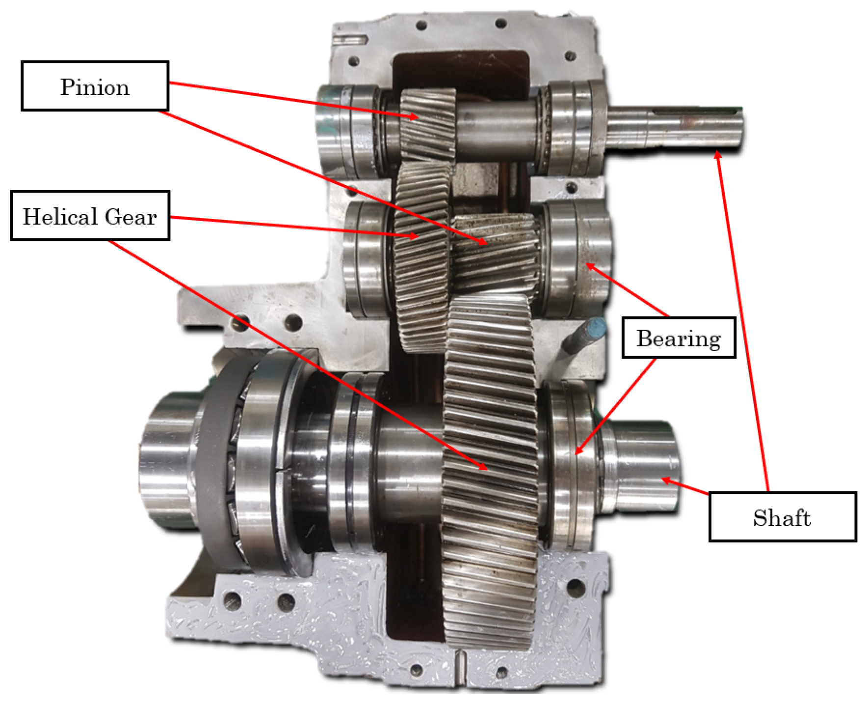
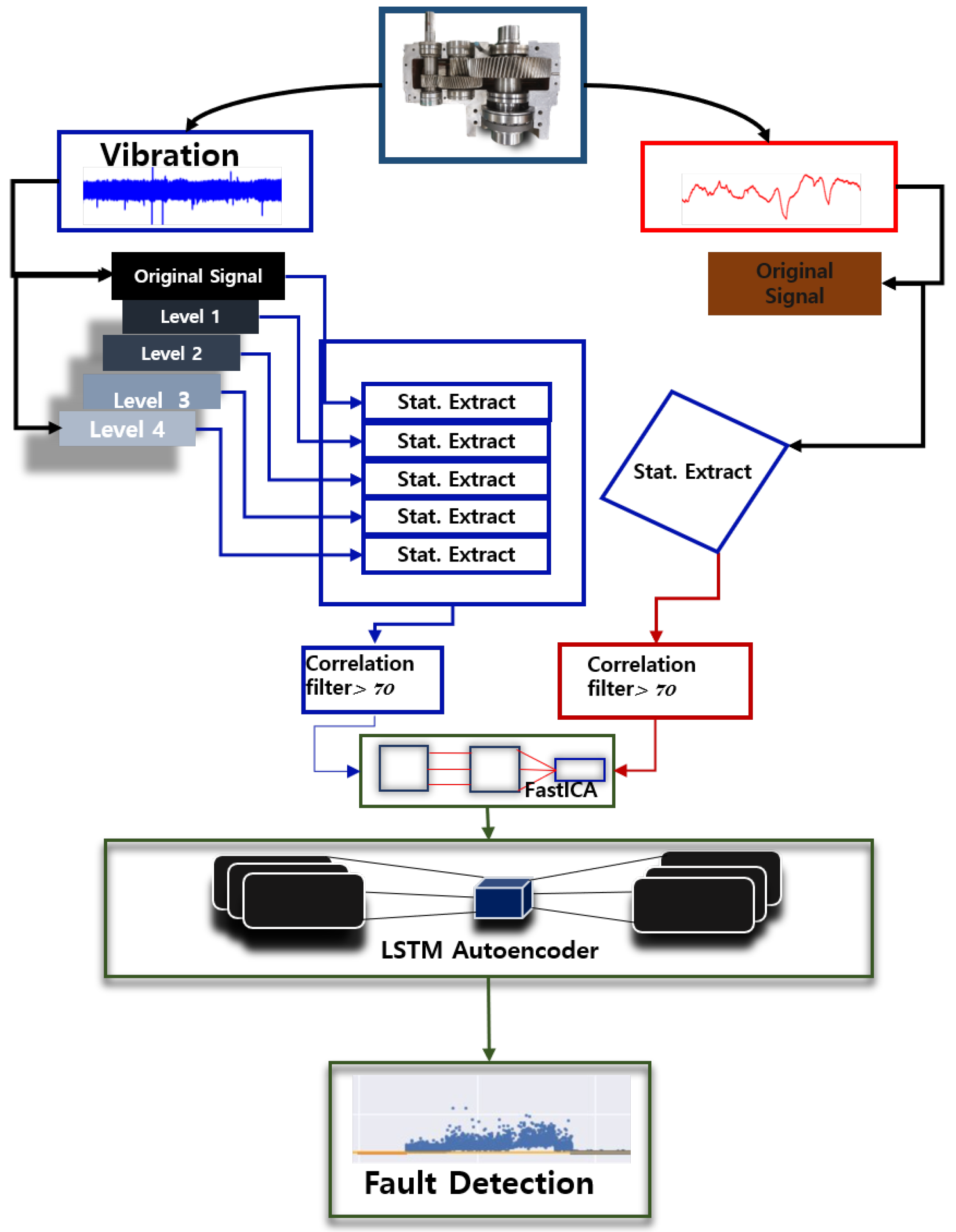
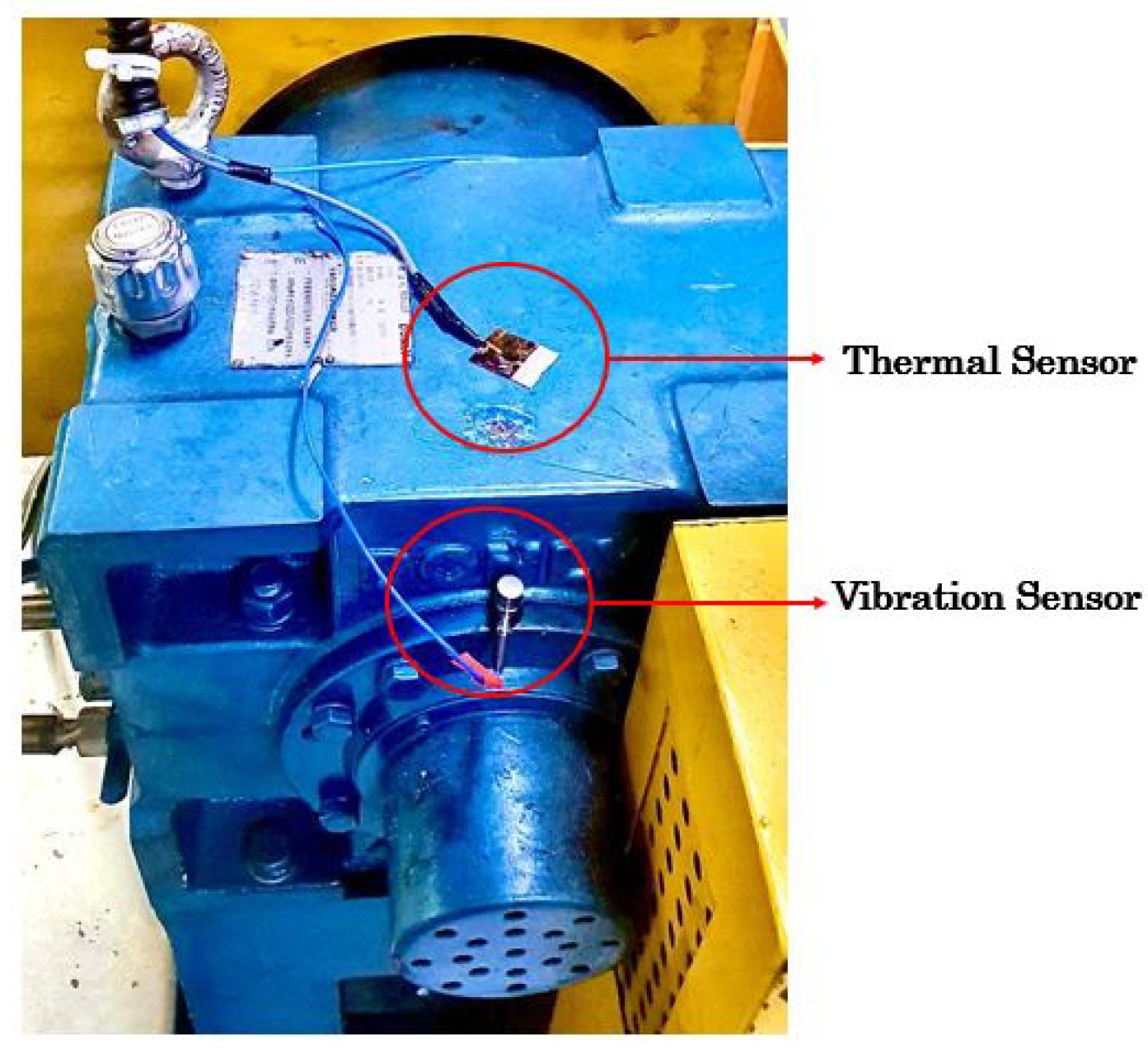
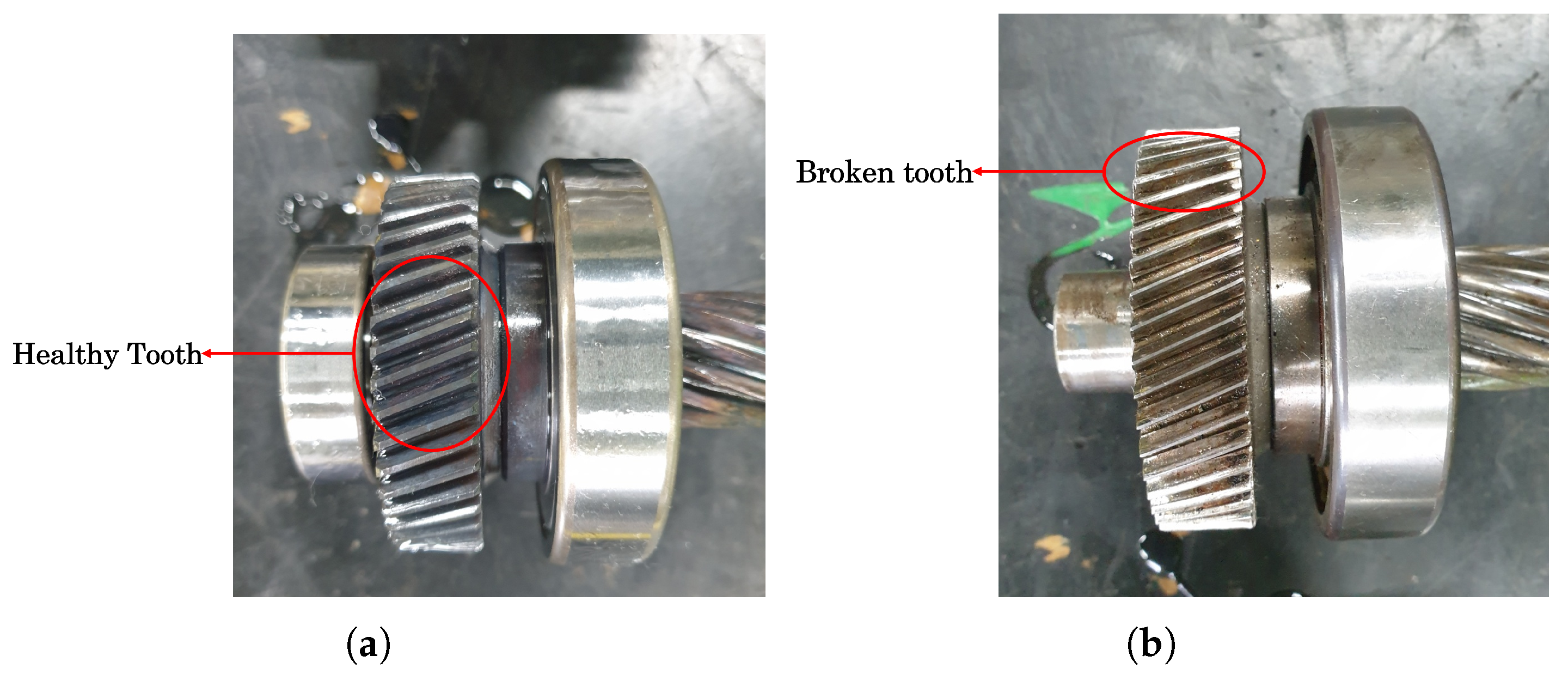
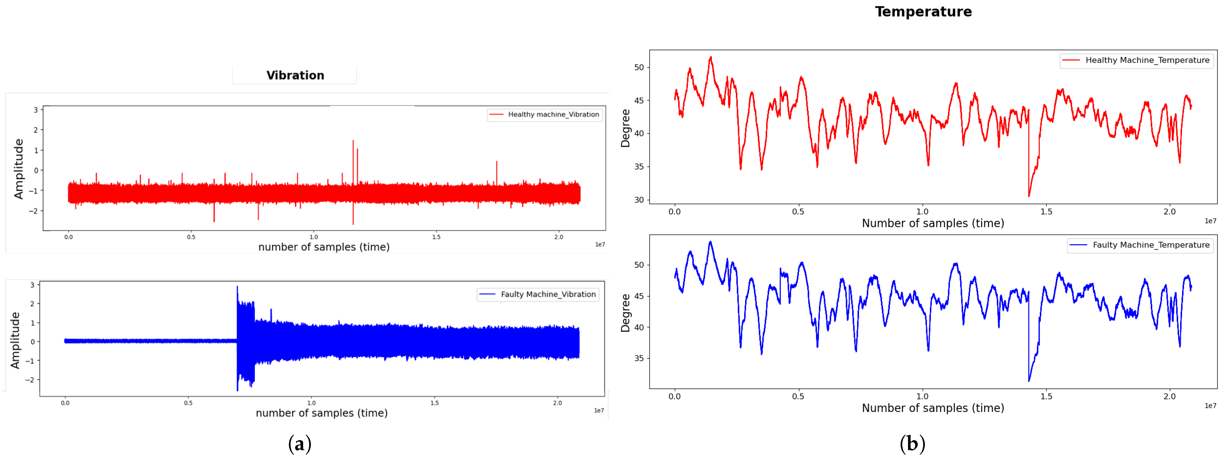
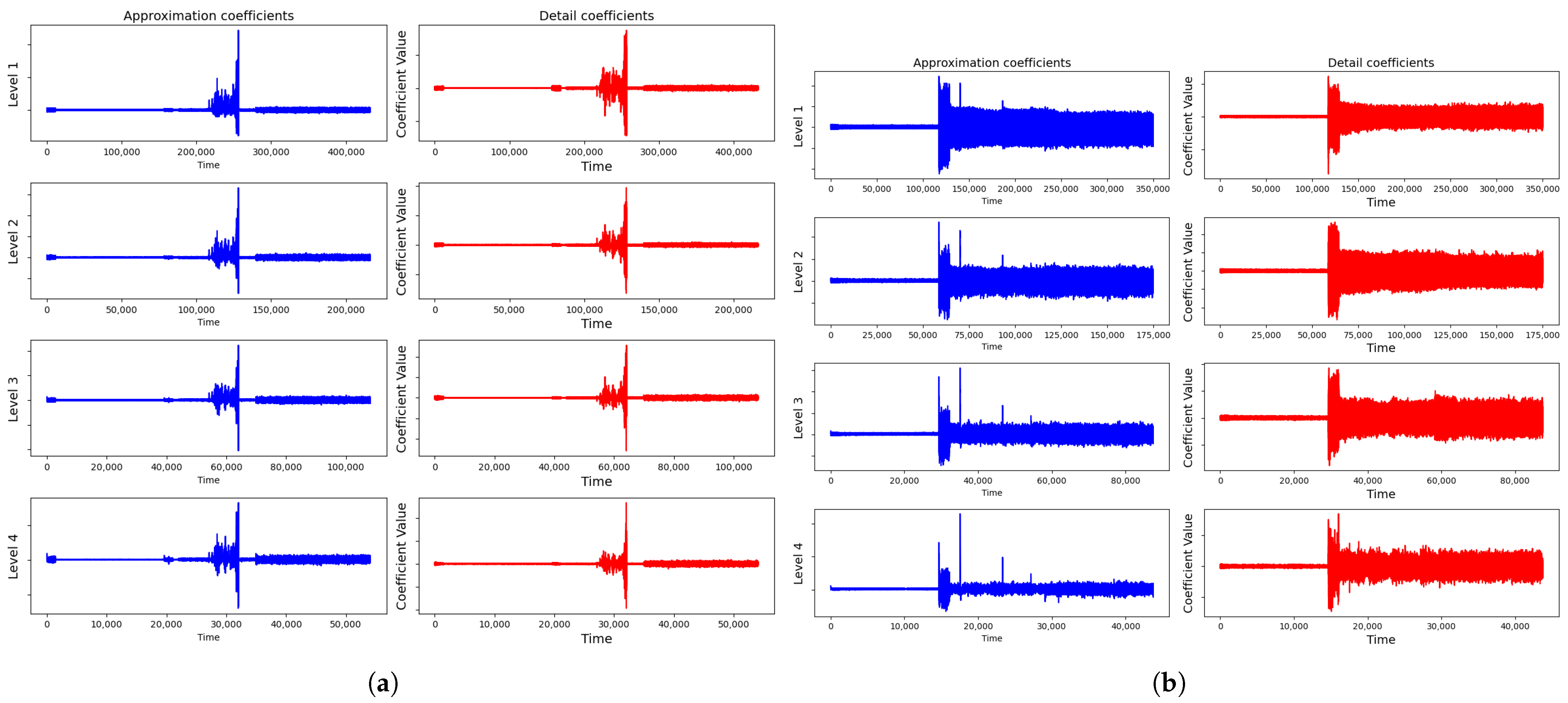
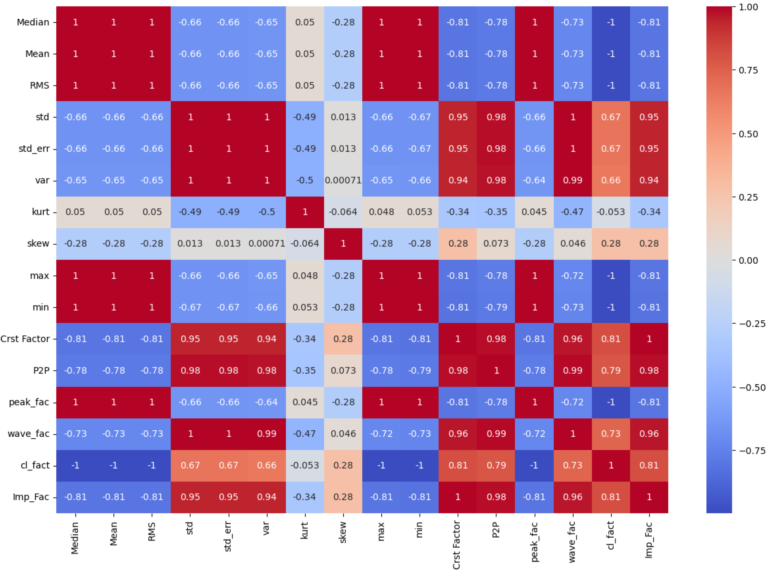
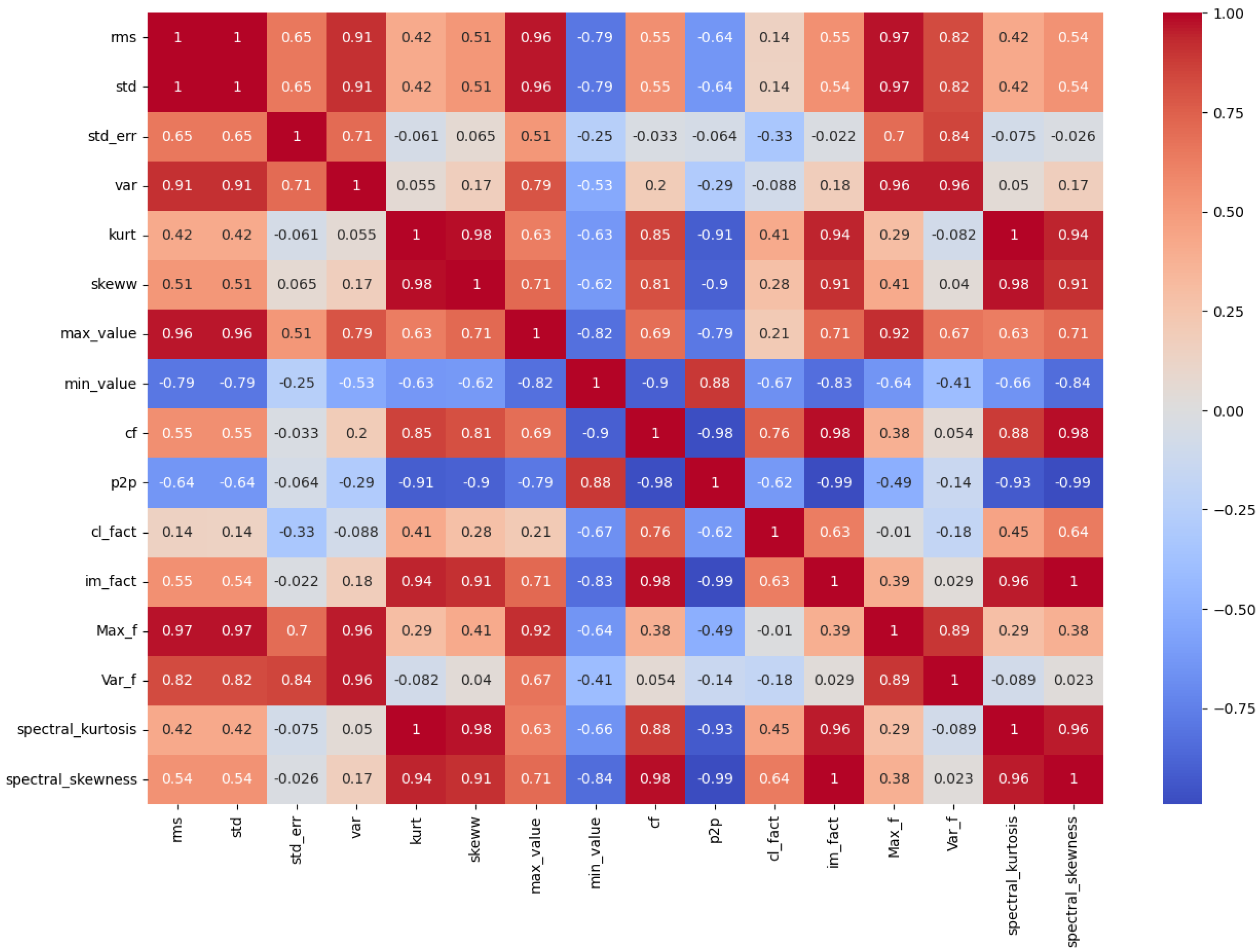
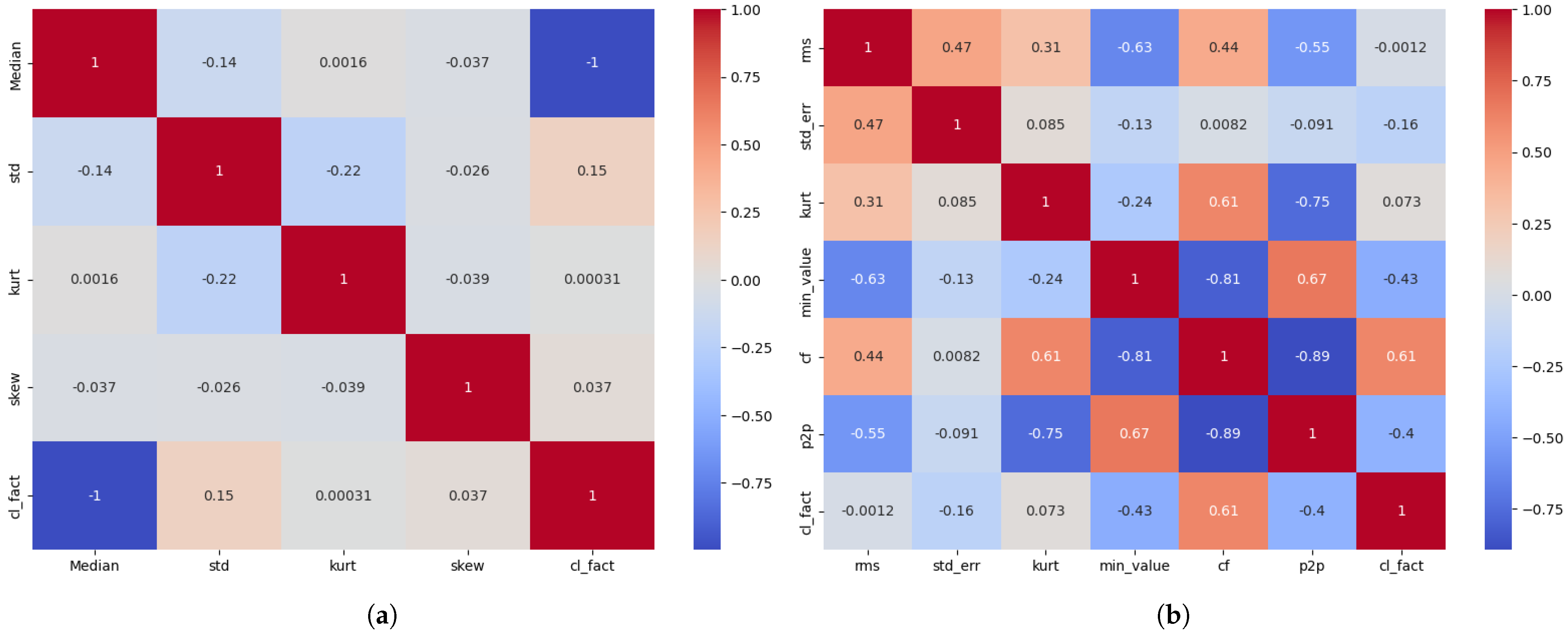
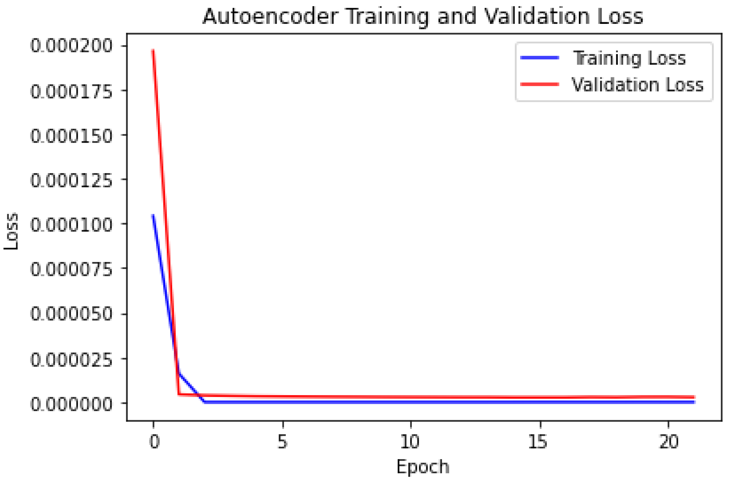
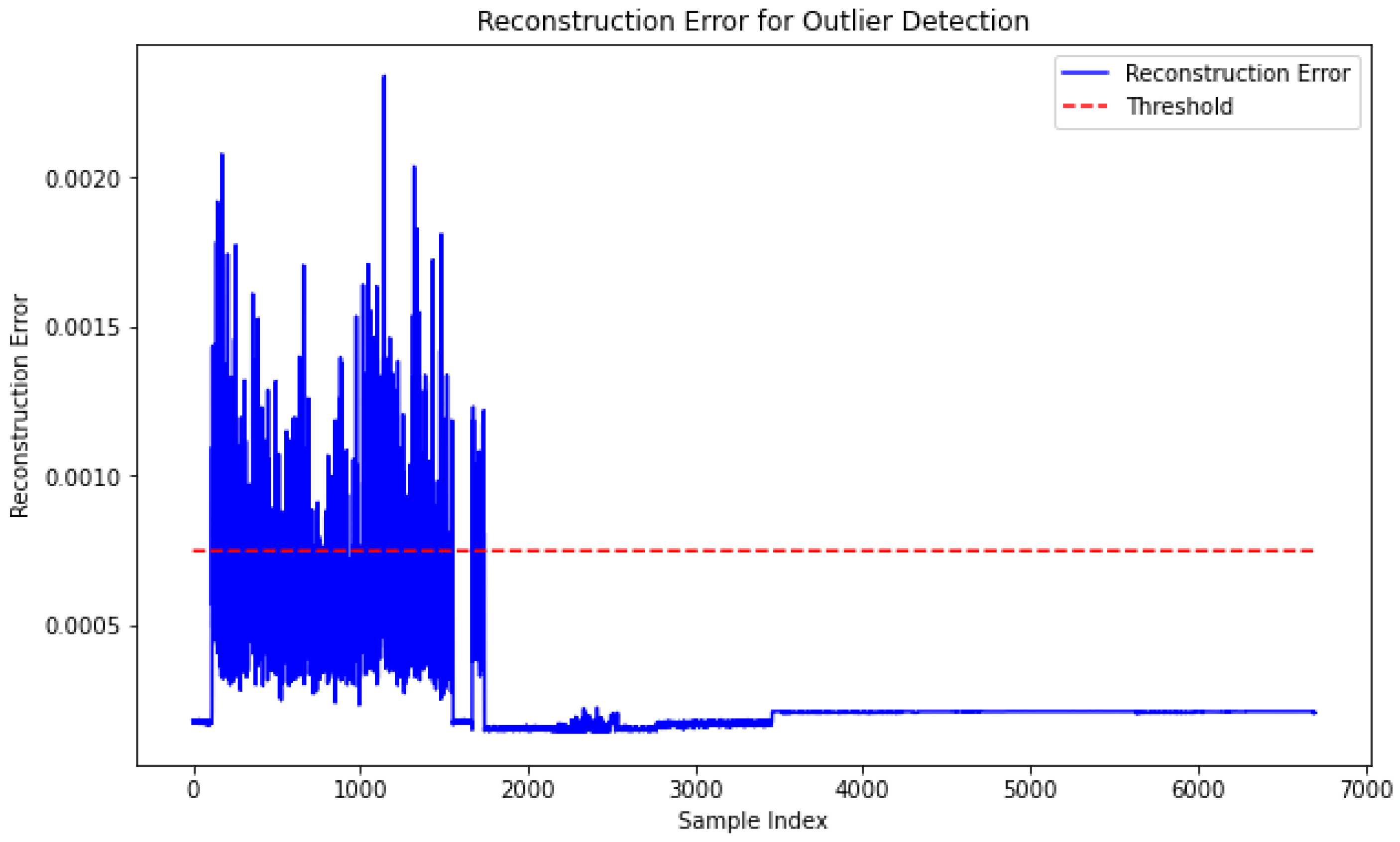
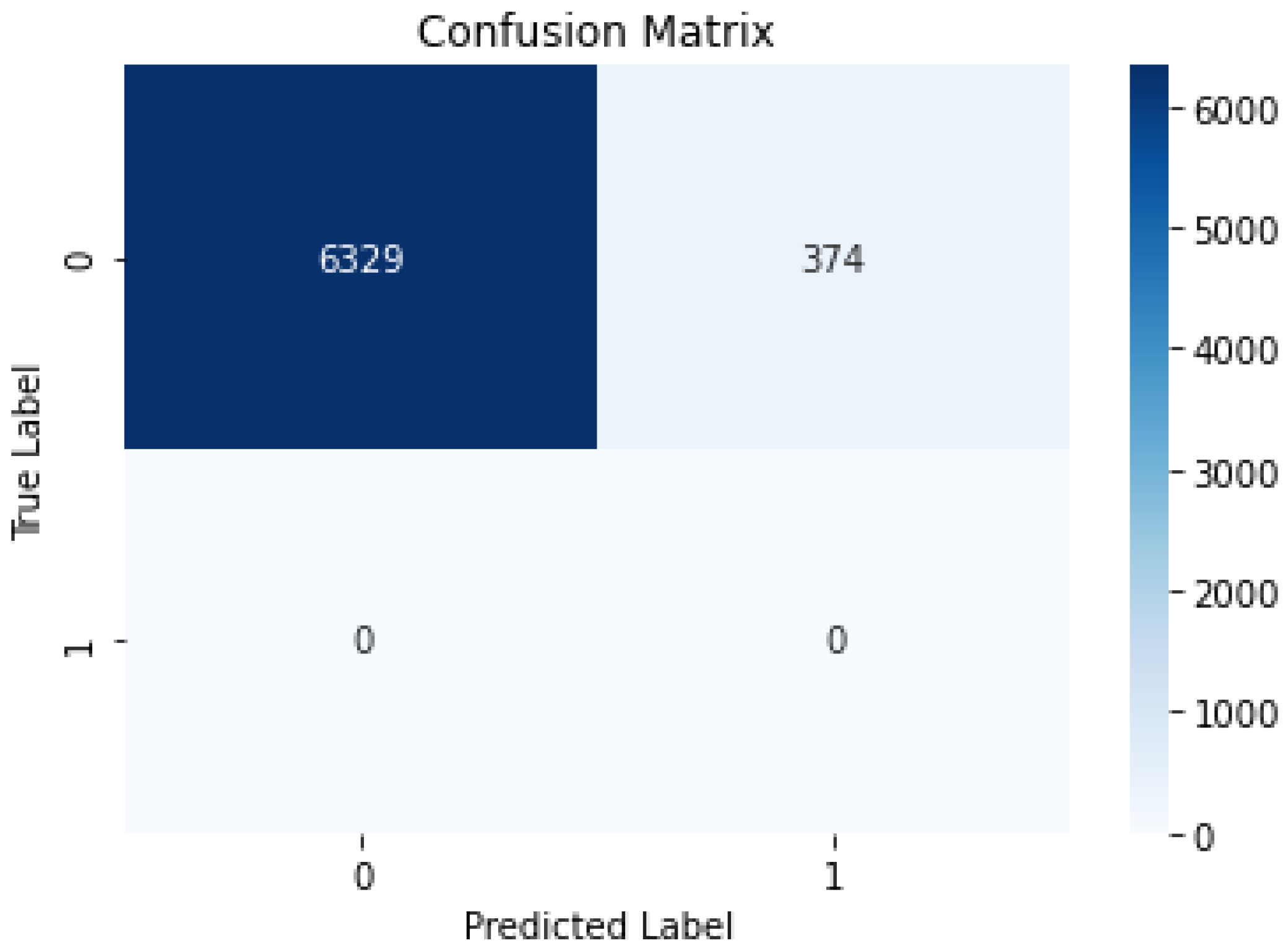
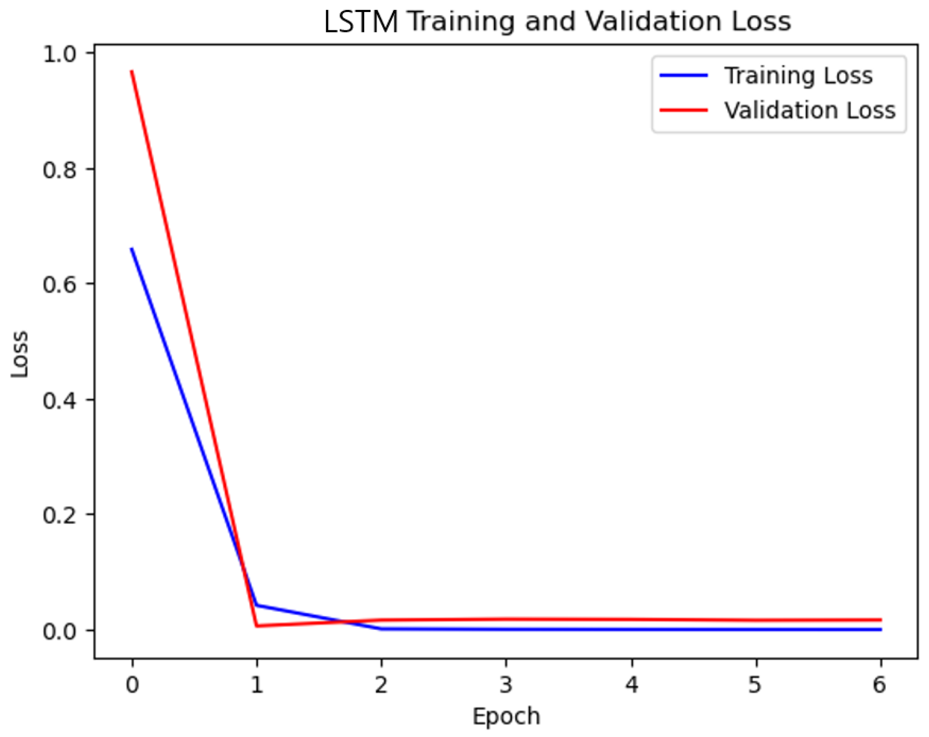
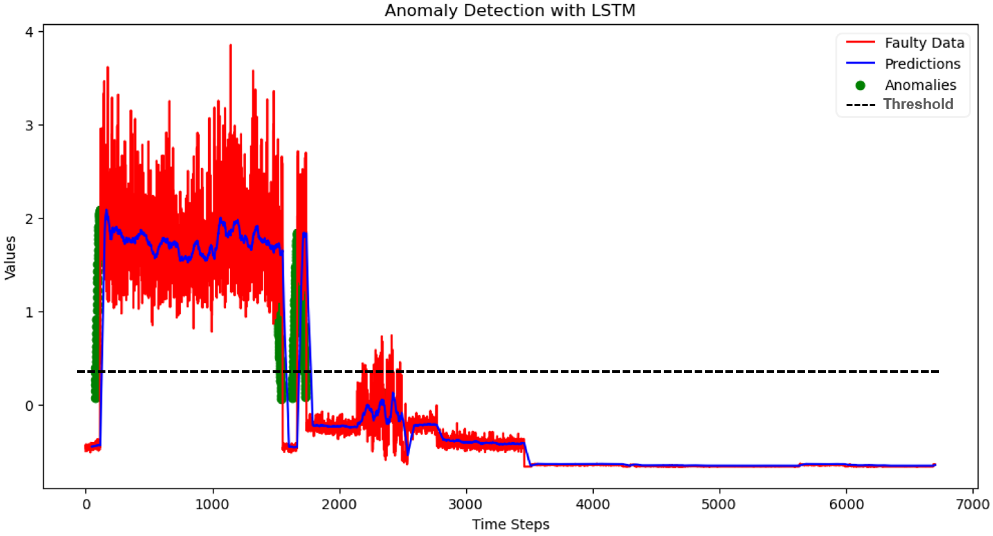
Table 1.
AE-LSTM Architecture Model Parameter.
| Model Architecture | Description |
|---|---|
| Number of Classes | 2 |
| Number of Layers | 7 |
| Batch Size | 32 |
| Number of Epochs | 100 |
| Dropout Rate | 0.001 |
| Optimizer | Adam |
| Activation Function | Relu |
| Loss Function | MSE |
| Validation Split | 0.2 |
Table 2.
Statistically extracted features and their mathematical formulas.
| Domain | Feature Name | Definition |
|---|---|---|
| Time-Domain | Median | sample |
| Mean | ||
| Root Mean Square | ||
| Standard Deviation | ||
| Variance | ||
| Standard Error | ||
| Kurtosis | ||
| Skewness | ||
| Max | ||
| Min | ||
| Crest Factor | ||
| Peak-to-peak | ||
| Peak factor | ||
| Wave Factor | ||
| Clearance factor | ||
| Impulse factor | ||
| Frequency-Domain | Maximum Frequency | |
| Variance Frequency | ||
| Spectral Kurtosis | ||
| Spectral Skewness |
Table 3.
Global Evaluation Metrics values for the AE-LSTM Model.
| Definition | Accuracy (%) | Precision (%) | Recall (%) | F1-Score (%) |
|---|---|---|---|---|
| AE-LSTM | 94.42 | 100 | 93.67 | 91.72 |
Table 4.
LSTM Architecture Model Parameter.
| Model Architecture | Description |
|---|---|
| Number of Classes | 2 |
| Number of Layers | 4 |
| Batch Size | 64 |
| Number of Epochs | 20 |
| Optimizer | Adam |
| Activation Function | Sigmoid |
| Loss Function | MSE |
| Validation Split | 0.2 |
Table 5.
Global Evaluation Metrics values for the LSTM Model.
| Definition | Accuracy (%) | Precision (%) | Recall (%) | F1-Score (%) |
|---|---|---|---|---|
| LSTM | 89.67 | 98 | 88.01 | 86.31 |
Disclaimer/Publisher’s Note: The statements, opinions and data contained in all publications are solely those of the individual author(s) and contributor(s) and not of MDPI and/or the editor(s). MDPI and/or the editor(s) disclaim responsibility for any injury to people or property resulting from any ideas, methods, instructions or products referred to in the content. |
© 2023 by the authors. Licensee MDPI, Basel, Switzerland. This article is an open access article distributed under the terms and conditions of the Creative Commons Attribution (CC BY) license (https://creativecommons.org/licenses/by/4.0/).
Share and Cite
MDPI and ACS Style
Lee, J.-H.; Okwuosa, C.N.; Hur, J.-W. Extruder Machine Gear Fault Detection Using Autoencoder LSTM via Sensor Fusion Approach. Inventions 2023, 8, 140. https://doi.org/10.3390/inventions8060140
AMA Style
Lee J-H, Okwuosa CN, Hur J-W. Extruder Machine Gear Fault Detection Using Autoencoder LSTM via Sensor Fusion Approach. Inventions. 2023; 8(6):140. https://doi.org/10.3390/inventions8060140
Chicago/Turabian StyleLee, Joon-Hyuk, Chibuzo Nwabufo Okwuosa, and Jang-Wook Hur. 2023. "Extruder Machine Gear Fault Detection Using Autoencoder LSTM via Sensor Fusion Approach" Inventions 8, no. 6: 140. https://doi.org/10.3390/inventions8060140