IIR Shelving Filter, Support Vector Machine and k-Nearest Neighbors Algorithm Application for Voltage Transients and Short-Duration RMS Variations Analysis

Abstract

This paper focuses on both voltage transients and short-duration RMS variations, and presents a unique and heterogeneous approach to their assessment by applying AI tools. The database consists of both real (obtained from Lithuanian PQ monitoring campaigns) and synthetic data (obtained from the simulation and literature review). Firstly, this paper investigates the fundamental grid component and its harmonics filtering with an IIR shelving filter. Secondly, in a key part, both SVM and KNN are used to classify PQ events by their primary cause in the voltage–duration plane as well as by the type of short circuit in the three-dimensional voltage space. Thirdly, since it seemed to be difficult to interpret the results in the three-dimensional space, the new method, based on Clarke transformation, is developed to convert it to two-dimensional space. The method shows an outstanding performance by avoiding the loss of important information. In addition, a geometric analysis of the fault voltage in both two-dimensional and three-dimensional spaces revealed certain geometric patterns that are undoubtedly important for PQ classification. Finally, based on the results of a PQ monitoring campaign in the Lithuanian distribution grid, this paper presents a unique discussion regarding PQ assessment gaps that need to be solved in anticipation of a great leap forward and refers them to PQ legislation.

1. Introduction

Nowadays, greater and greater integration of artificial intelligence (AI) into the modern world is observed. Electric power systems together with power quality (PQ) application are not an exception. A state-of-the-art review [1] (2015) on both signal processing and AI techniques application in the classification of PQ disturbances distinguishes the following stages of the process:

• Input data stage. It is obvious that the quality of machine learning is directly related to input data which is closely related to algorithms used and tasks undertaken. However, discussion on these aspects is skipped in [1]: in our opinion, one of the reasons (for that skipping) can be the deficiency of PQ monitoring systems at that time [2]. In this paper, initial data gathering is described in Section 2.1.
• Feature extraction stage. The following taxonomy of the techniques is given in [1]: Fourier transform, Kalman filter, wavelet transform, S-transform, Hilbert–Huang transform, Gabor transform, and miscellaneous or less often used (e.g., time–frequency representation, Teager energy operator, etc.). A result of classification highly depends on both the features selection strategy and their extraction accuracy.
• Classification stage. The following tools are highlighted in [1]: artificial neutral network, support vector machine, fuzzy expert system, and miscellaneous (e.g., k-nearest neighbors).
• Feature selection and parameter optimization stage. In this stage, the redundant features with low recognition rate are discarded. The following tools for selection of the best suitable feature subset are highlighted in [1]: genetic algorithms, particle swarm optimization, and ant colony optimization.
• Decision stage. Discussion on this topic is also skipped in [1]: in our opinion, one of the reasons can be that a practical significance of many research studies (algorithms) is insufficient and more comprehensive investigations (technical progress) are required for their commercialization and application in electric power systems.

The authors of [1], as can be noticed from their paper title, treat signal processing and AI algorithms as two separate fields. This is because, especially in the business world, AI is mostly associated with machine learning using the most well-known tools such as neural networks. However, if examined more deeply, the philosophy of AI is not so primitive, and the absence of a unified and simple definition accompanies it throughout the entire timeline of evolution of intelligence and thinking. Its origin dates back to the invention of writing, with the earliest known libraries on clay tablets in Mesopotamia (initially under the control of Sumerians and Akkadians, later ceded to such famous states as the Old Babylonian Empire, Assyrian Empire and New Babylonian Empire, and then followed by the defeat to Achaemenid Persian Empire) as well as in other places in particular cradles of civilization such as ancient Egypt, Indus Valley Civilization, and ancient China, later followed by Greek mythology which includes the idea of artificial beings and intelligent machines such as Talos (a giant bronze automaton made to protect Europe in Crete) [3]. At this point, we mentioned the term of ‘automaton’, a relatively self-operating machine, the first form of robot, which seems to be invented by ancient Egyptians: their statues of gods “spoke, moved, acted—not metaphorically, but actually”, for example, replying to each question by a movement of the head [3,4,5]. Aristotle speculated in his Politics [6] (book 1, part 4) about automata as a mean for abolitionism: “For if every instrument could accomplish its own work, obeying or anticipating will of others, like the statues of Daedalus, […] if, in like manner, the shuttle would weave and the plectrum touch the lyre without hand to guide them, chief workmen would not want servants, nor masters slaves”. His syllogisms for proper reasoning are also worth mentioning, because this highly contributed to the development of logic which is an indispensable part of AI [3,7]. To continue, the prohibition against making graven images (the second commandment), taking place in the desert of Sinai, is also discussed in [3] through a prism of AI. When the discussion comes to medieval and early modern periods, the following achievements should be highlighted: (1) the flourishing of Arab mathematics and science (e.g., zairja—a device for ideas generation by mechanical means) during the Golden Age of Islam, and these ideas transferring to Europe (via Spain, Sicily, and Crusader kingdoms in the Levant); (2) appearance of mechanical clocks, the first modern measuring machine, in European towns (15th–16th centuries); (3) invention of a mechanical calculator, the Pascaline, by Blaise Pascal; (4) philosophy and other scientific contributions of René Descartes (e.g., rationalism, mind–body dualism, Cartesian coordinate system, etc.) [3]. Obviously, it is impossible to encompass (classify) all important milestones in one paragraph; hence, many contributions remain unmentioned, in particular outside Europe and the Middle East. The scientific revolution (Nicolaus Copernicus’ publication on the heliocentric theory (in 1543) is often considered as its beginning, while Isaac Newton’s publication on the laws of motion and universal gravitation (in 1687) is considered as its culmination) and the Age of Enlightenment (17th–18th centuries) followed by the First Industrial Revolution laid the foundation for further acceleration in the development of science in the late modern period. Moreover, science fiction did not disappear with such works as Hoffman’s The Sandman, Goethe’s Faust, and Mary Shelley’s Frankenstein [3].

The history of modern AI began in the mid-20th century with such achievements as cryptanalysis of the Enigma (which enabled Allies to read considerable amounts of Morse-coded messages of Axis power), the Turing test (a method to determine whether a machine can demonstrate human intelligence), checkers (draughts) and chess engines [3,7], i.e., before AI commercialization (which, according to [3], begun after 1980) and large-scale application of artificial neural networks. Currently, the following major concepts of AI are often distinguished in the literature: (1) artificial general intelligence (or strong AI), and (2) artificial narrow intelligence (or weak AI) [8]. Also, other categories can be found such as generative AI or symbolic AI; however, detailed analysis of this field is outside the scope of this paper. According to [7], most researchers “take the weak AI hypothesis for granted”, and do not care about the general intelligence; however, “all AI researchers should be concerned with the ethical implications of their work”. The field of electric power systems, including its PQ application and this paper, is not an exception. In the PQ field, a wide-ranging implementation of AI may be expected; however, at the moment, the suitability of many AI algorithms still remains insufficiently explored [2]. In this paper, the small paragraph of scientific achievements of earlier times is given not without reason—all ideas (approaches) are potentially suitable (beneficial) for joint PQ and AI research. For example, the usage of logical reasoning in the field of PQ to discuss the results obtained can be found in [9]. Soft skills and philosophical insights during results interpretation are just as important as software code writing; thus, it is inseparable from the knowledge in philosophy, development of scientific ideas and their spread, etc. Ideally, for use in practice, an AI algorithm may be multicriterial and based on a complex mathematical apparatus, but simultaneously, it should have such features as simplicity, understandability, sufficient accuracy, time efficiency, cost efficiency, etc. In the case of embedded systems, algorithms must also be resource saving to avoid an undesirably fast runoff of the battery. Moreover, it is not a secret that sometimes, the conclusion about the accuracy of the developed algorithm can be limited (incorrect), because either the training data set or validation (test) data set may not represent its population sufficiently enough. In PQ papers, the risk of such or similar limitations is inevitable and cannot be fully eliminated. For example, in the case of the PQ monitoring allocation task, the size of the test schemes used is mostly up to 123 buses (IEEE test scheme); therefore, it remains unclear whether any proposed algorithm will be suitable for a large power system [2]. In addition, in our opinion, each paper should discuss in which structural part of the PQ monitoring process a proposed algorithm can be used (see [2] for the general structure of a remote PQ monitoring process).

Each PQ research should be started from the definition of target PQ events [2]. The target group of this paper consists of both transients and short-duration RMS variations. The next stage should be a selection of both features and algorithms. Let us begin the literature review with the PQ standards, because they include (reflect) universally agreed (applied) approaches. Firstly, in the case of transients, there are almost no requirements for both measurement and assessment in IEC 61000-4-30:2015 [10]. On the other hand, this standard provides ideas about transient voltage detection by the comparative method, envelope method, sliding-window method, etc. When the event is detected by either method, the following list of classification methods and parameters is given: peak value, overshoot voltage, the rate of rise (i.e., the first time derivative of either voltage or current) of the leading edge, frequency parameters (spectrum), duration, damping coefficient, frequency of occurrence, energy and power (available or conveyed), and continuity type (continuous or single-shot transient). EN 50160:2010 [11] does not provide any noteworthy information about transients nor does it establish the norms. IEEE Std 1159-2019 [12] uses the rise time, duration, spectral content and magnitude, and it also gives additional hints for the characterization of transient energy, direction, form (e.g., positive, negative, unipolar, bipolar, oscillatory, multiple-zero crossing). Secondly, in the case of voltage sags, IEEE Std 1564-2014 “Guide for Voltage Sag Indices” [13] proposes a voltage sag energy index and voltage sag severity index (using SEMI F47 curve as a reference), along with the other useful information regarding both site and system indices, which are not relevant to the scope of this paper. Meanwhile, IEC 61000-4-30:2015 states that “depending on the purpose of the measurement, other characteristics in addition to depth and duration should be considered” and presents the following ideas: voltage sag unbalance, phase angle of the beginning, phase shift, missing voltage, voltage sag distortion (e.g., estimated by total harmonic distortion—THD). EN 50160:2010 along with IEEE Std 1159-2019 use only voltage and duration. The voltage–duration plane is undoubtedly the most preferred and best understood method which, for example, has hegemony in such areas as the settings of relay protection and automation, equipment immunity testing, and fault-ride-through requirements.

PQ events classification is not an extremely recent research field. For example, [14] (2001) proposes a voltage sag classification and characterization method based on fuzzy logic: (1) voltage sags are classified into three groups—caused by grid fault, large motor starting, and interaction between motor operation and grid fault; (2) three features are extracted from the simulated voltage waveforms—phase angle shift, duration, and voltage change. As has been mentioned above, earlier achievements are a necessary prerequisite for modern research: for example, it can be highlighted that the k-nearest neighbors algorithm was firstly developed in 1951 [7], but it will still be investigated in this paper. The state-of-the-art of the joint PQ and AI field until 2015 is more or less reviewed by [1] (2015). Then, for example, [15] (2016) investigates the application of optimal multi-resolution fast S-transform along with classification and regression tree. The following PQ disturbances and their combinations have been generated by the simulation: transient, interruption, sag, swell, flicker, harmonics, and six their combinations—transient with sag, transient with swell, transient with flicker, sag with harmonics, swell with harmonics, and flicker with harmonics. The selected features—statistical parameters (maximum, minimum, standard deviation, skewness, kurtosis, etc.) and energy—are extracted from the simulated voltage waveforms. Next, [16] (2020) reviews the state-of-the-art of PQ events detection and classification until 2020. Feature extraction techniques are grouped into Fourier transform—FT (including its well-known variants: discrete-time Fourier transform—DTFT, fast Fourier transform—FFT, and short-time Fourier transform—STFT), S-transform—ST, Hilbert–Huang transform—HHT (including empirical mode decomposition—EMD), wavelet transform—WT (including tunable Q-factor wavelet transform—TQWT), and miscellaneous techniques (e.g., Gabor transform—GT, optimal feature selection based on ant colony optimization—ACO, etc.). Also, the following AI techniques, used in the PQ events detection and classification, are discussed: support vector machine—SVM (including its multiclass extension—MSVM), artificial neural network—ANN (including the following types: feedforward neural network—FNN, probabilistic neural network—PNN, recurrent neural network—RNN), fuzzy logic—FL, neuro-fuzzy system—NFS, genetic algorithm—GA, deep learning-based methods (convolutional neural network—CNN, long short-term memory—LSTM), and miscellaneous (e.g., extreme learning machine—ELM, particle swarm optimization—PSO, etc.). In addition, the paper categorizes the data used by type (synthetic or real), also—whether their data were noisy or noiseless. Many authors prefer to analyze their initial data with additionally injected noise (e.g., white noise), which can be quantified by the signal-to-noise ratio (SNR). To continue, the list of the reviewed newest papers [17,18,19,20,21,22,23,24,25,26,27,28,29,30,31,32,33,34,35,36,37,38,39], which are more or less relevant to the scope of this paper, is given in

Table 1. Highlights of the newest reviewed and relevant papers.

Reference 1	Algorithm 2	Task 3	Target Group 4					Data 5	Parameters, Features
[17] (2023)	ST, RF	C	ImT		OsT	Int	Sg	S, R	Maximum magnitudes (peaks) of FFT spectrum of the signal 6
			Sw	F	H	N	C
[18] (2023)	CNN-LSTM	C, S 7	ImT		OsT	Int	Sg	S	Deep features of 1D time series signal 8
			Sw	F	H		C
[19] (2023)	DT, KNN, RF, SVM, VAE	C, L 9					Sg 10	S 11	Current, voltage, fault type and location
			Sw 10
[20] (2023)	CNN, ST	C	ImT	Sp 12	OsT	Int	Sg	S, R	Deep features of 2D time–frequency matrix
			Sw	F	H	N	C
[21] (2023)	OFDT, PCA	C		Sp	OsT	Int	Sg	S	Power spectrum estimated by Welch’s method
			Sw	F	H	N
[22] (2023)	CNN, HT	C	ImT		OsT	Int	Sg	S, R 14	Deep features of voltage amplitude envelope
			Sw	F 13	H	N	C
[23] (2022)	Not applicable	A					Sg	S	Voltage, time, energy index, influence degree (severity)
			Sw
[24] (2022)	Fast SVM	C				Int	Sg	S	The input is the amplitude of one cycle of the distorted wave
			Sw		H		C
[25] (2022)	2D WT, CNN 15	C	ImT		OsT	Int	Sg	S	Deep features of the colored image of the time–frequency plane
			Sw
[26] (2022)	LSTM	C	ImT	Sp	OsT	Int	Sg	S	The input is the raw sample with its PQ event type
			Sw	F	H	N	C
[27] (2022)	DT, KNN, LR, RF, SVM	L					Sg 10	S, R	28 features extracted from voltage and current waveforms 16
			Sw 10
[28] (2022)	WT	F					Sg	S	Voltage, time, cross-correlation coefficients with mother wavelets
[29] (2022)	TQWT 17	C	ImT		OsT	Int	Sg	S	Statistical parameters, sub-band energy ratio, zero crossings, etc. 18
			Sw	F	H	N	C
[30] (2022)	LSTM	C					Sg	S, R	Voltage, fault type 19
[31] (2021)	CT	C					Sg	S	Clarke components ellipse
[32] (2021)	FNN	C		Sp	OsT	Int	Sg	S	Binary image of PQ signal waveform and its saliency map
			Sw	F	H	N	C
[33] (2021)	ABC-PSO, MRA, PNN, WT	C	ImT	Sp	OsT	Int	Sg	S	Energy, entropy, standard deviation, mean and other statistical parameters
			Sw	F	H	N	C
[34] (2020)	EM, GA, SVM 20	L					Sg 10	S	34 features extracted from voltage and current waveforms 16
			Sw 10
[35] (2020)	DT, ST	C			OsT	Int	Sg	S, R	Maximum amplitude versus both time and frequency, THD, etc.
			Sw	F	H		C
[36] (2020)	MLP, SVM	C					Sg 21	S	Higher-order statistics (moments and cumulants), cause
[37] (2020)	CSO, DT, GA, KNN, ST, SVM	C	ImT		OsT	Int	Sg	S	Statistical parameters, disturbance energy ratio
			Sw	F	H	N	C
[38] (2019)	ELM, WT	C		Sp	OsT	Int	Sg	S, R	Statistical parameters, wavelet coefficients
			Sw	F	H	N	C
[39] (2019)	ST	F					Sg 22	S	First and second duration times, recovery time and magnitude, THD 23

¹ Year of publishing online (acceptance) is given in the brackets, which does not necessarily coincide with a year of scientific journal. ² In this column, more generic names are given, which not always reflect developed (proposed) modifications by various authors. Moreover, they are not classified by purpose (e.g., for feature extraction, feature optimization, classification, etc.). ³ Type of the task: A—impact assessment, C—classification, F—feature extraction (characterization, also may be detection), L—localization, S—cybersecurity. ⁴ PQ events: ImT—impulsive transient, Sp—spike, OsT—oscillatory transient, Int—interruption, Sg—sag, Sw—swell, F—flicker, H—harmonics, N—notching, C—combination of multiple events. ⁵ Data acquisition method: S—synthetic, R—real. ⁶ Many not widely known challenges (issues) are present during the analysis of frequency domain. Some of them are discussed (mentioned) in both this and Section 4.3.1. ⁷ The defense of the classifier from an adversarial attack is investigated. ⁸ Deep features are complex patterns extracted from the intermediate layers of CNN. ⁹ The distance (location) is expressed in numbers. ¹⁰ All four types of short circuit are encompassed. ¹¹ The original data set had been obtained by simulation, and then, it was synthetically enlarged with VAE. ¹² Despite the fact that a spike is not included in the PQ legislation, authors sometimes prefer to distinguish it from impulsive transient. ¹³ Called as fluctuation. ¹⁴ Real data were generated by the programmable AC power source. ¹⁵ Generalized Morse, analytic Gabor and bump wavelets are investigated. ¹⁶ Papers [27,34] are kindred, including the features used by them. These features are obtained from many earlier papers and are based on various manipulations with different electrical parameters such as current, apparent power, reactive power, power factor, etc. ¹⁷ TQWT is parameterized by $Q$, $r$ and $J$. ¹⁸ In this table, statistical parameters stand for well-known characteristics such as the mean, standard deviation, range, skewness, excess kurtosis, etc., including any manipulation (operation) with them. ¹⁹ The following parameters are required for voltage sag generation with the synthetic signal generator: signal duration, fault start time, fault duration, nominal RMS, signal frequency, sampling frequency, no-fault amplitude, phase angle offset, number of smoothing timepoints, fault severity, signal rotation, noise percentage, and the label (the type of the fault to be generated). ²⁰ The ensemble utilizes discriminant, KNN and DT weak learners (three learners, nine methods). ²¹ Three causes are included: fault, motor inrush current, and transformer inrush current. ²² The eight types (causes) are included: line to line fault, self-extinguishing fault, induction motor starting, transformer energizing, multistage fault, line fault before induction motor starting, line fault with harmonics caused by a single-phase nonlinear load, and multistage fault with harmonics caused by a single-phase nonlinear load. ²³ Several time parameters are required to characterize a duration of a multistage voltage sag (see Section 4.1).

. In addition to the already mentioned ones, the following AI tools can also be found in the table: artificial bee colony—ABC, competitive swarm optimization—CSO, Clarke transformation—CT, decision tree—DT, ensemble methods—EM, Hilbert transform—HT, k-nearest neighbors—KNN, logistic regression—LR, multilayer perception—MLP, multiresolution analysis—MRA, ordered fuzzy decision tree—OFDT, principal component analysis—PCA, random forest—RF, variational autoencoder—VAE. Also, many simpler ideas and operations such as normalization or other signal processing techniques are left behind.

PQ classification is the main objective of the most reviewed papers, but some other interesting instances are also given in this paper. These instances are related with the following tasks: cybersecurity, localization of PQ emission source (fault), impact assessment (e.g., damage to end-user equipment), and features extraction (also including characterization and detection). For example, the localization can be determined either qualitatively or quantitatively (Figure 1a): the identification of voltage sag source side (upstream or downstream) is a qualitative approach (see [9] for more information), while the estimation of a distance to the fault node in units of length is a quantitative approach (see [2] for more information about the case of PQ monitors displacement algorithms). Please note that the classification itself often includes a wider range of tasks such as an event detection and features extraction. The proposed concept of interconnection between PQ event localization and classification is shown in Figure 1b. For example, the identification of voltage sag side can also be considered as a kind of classification by fault location (e.g., TSO grid, DSO grid, in-plant grid), and such an approach should be important in anticipation of responsibility sharing and penalties. In the most reviewed papers (especially with a wider target group), the classification is performed by a PQ event; however, it must be performed not only by a PQ event which is really more about its detection and recognition, but also by its type or its primary cause. For example, in this work, transients are classified by their primary cause (commutation or atmospheric), and short circuits are classified by their type (three-phase, two-phase-to-ground, two-phase, and single-phase). However, currently, there is a lack of research (data) about primary causes of PQ events [9].

To continue, in most of the papers reviewed, the main data generation method is synthetic, which sometimes is supplemented with real measurements. In these papers, the creation of a synthetic database often is based on the mathematical models of PQ disturbances (parametric equations), which can be found in [40]: impulsive transient, spike, oscillatory transient, interruption, sag, swell, flicker, harmonics, notching, interruption with harmonics, sag with harmonics, swell with harmonics, flicker with sag, and flicker with swell. This is the reason why a spike appears in the target groups (see Table 1) despite being not included in PQ legislation. It was noticed that many reviewed papers are kindred—the usage of the same PQ events models from [40] leads to a loss of uniqueness. This paper does not use these equations. Also, it remains unclear what influence the relevant aspects of Section 4.1, which is based on the PQ monitoring campaign in the Lithuanian DSO grid, have on AI performance.

It must be highlighted that many authors boast about the very high classification accuracy achieved by their algorithms: for example, under different noisy environments, the declared classification accuracy is 99.4–100% in [17], 93.3–100% in [20], etc. Nevertheless, neither these nor other PQ classifiers are currently used in practice. In our opinion, in anticipation of a great leap forward in the PQ field, authors should be more honest (transparent) and discuss the limitations of their methods and approaches (e.g., as seen in Section 4.1). The authors sometimes also highlight further development avenues: for example, [20] mentions light-weighted optimization required for deploying the algorithm in embedded systems and also online training of its PQ classification model. A great diversity of feature extraction approaches can also be noticed in Table 1, and all currently investigated techniques has a potential for wide usage in the future. Despite the remarkable contribution, this area presently is still open [2], not commercialized and not applied in practice. Various techniques are applied in the feature selection and optimization stage: for example, [19] uses a customized version of forward feature selection (an iterative method starting with no features), and [33] uses adaptive ABC-PSO for optimal feature selection. The frequency domain is often studied as well—authors must pay attention (and sometimes do) to various encountered (and not always widely known) challenges such as Heisenberg uncertainty, window function and size, spectral leakage, spectral aliasing, etc. For example, [21] uses Welch’s method, which is beneficial for the noise reduction injected by the windowing of the overlapping segments of the power density spectrum. Furthermore, PQ signals can be analyzed either with or without the fundamental grid frequency component included [12]; however, despite the fact that some graphs are filtered in IEEE Std 1159-2019, other examples of such filtering were not found in the PQ literature.

The main method of analysis of this paper uses the voltage–duration plane: we will use the conventional approach and demonstrate that there are many unsolved questions. The main aim is to investigate the capabilities of both SVM and KNN to assess both transients and short-duration RMS variations, including both with the fundamental frequency component and filtered. Task No. 1 is to investigate the capabilities of the IIR shelving filter for 50 Hz and its harmonics filtering, task No. 2 is to investigate single-voltage classification in the voltage–duration plane, and task No. 3 is to investigate three-dimensional voltage classification. It goes without saying that the limitations of the research must also be discussed, and proposed ideas will be original and distinctive from the existing PQ literature as well as based on the PQ monitoring campaign in the Lithuanian DSO grid. But for now, let us begin from the first—input data—stage (Section 2.1).

2. Materials and Methods

2.1. Database

As has been mentioned in Section 1, each research on AI algorithms application should be started with a focus on the input data. The PQ data sources of this research are (1) the measurement campaigns in both the Lithuanian DSO grid and internal grids of industrial plants, (2) simulation with both MATLAB/Simulink and Siemens PSS/E software tool, and (3) literature analysis.

2.1.1. Commutation Transients

Voltage transients are classified into two categories—impulsive (non-oscillatory) and oscillatory. IEEE Std 1159-2019 divides each category further into three groups: (1) impulsive transients are classified by duration into nanosecond (less than 50 ns), microsecond (50 ns to 1 ms) and millisecond (longer than 1 ms); (2) oscillatory transients are classified by spectral content into low frequency (up to 5 kHz), medium frequency (5–500 kHz) and high frequency (0.5–5 MHz). Both categories of voltage transients are strongly interconnected because the electrical grid response to an impulsive transient can be oscillatory [12]. Meanwhile, EN 50160:2010 provides almost no information about voltage transients, and IEC 61000-4-30:2015 does not establish any measurement requirements. Moreover, measurement capabilities are limited not only due to the lack of the information but also due to technical issues related with measurement transducers (or, generally speaking, with measurement circuits)—for example, unknown magnitude and phase frequency response, or not having one voltage transformer installed in older substations (i.e., only two phase-to-ground voltages out of three are available to be measured). This is because the existing instrument transformers were designed only for fundamental frequency and electricity consumption metering—these issues have already been discussed in [2,9]. To continue, both sampling frequency and dynamic range aspects must also be considered. For example, approximately 200 MHz sampling is required to record 10 samples of 50 ns impulse, and 10 MHz sampling is required for a 5 MHz wave. The minimal requirement for sampling frequency, based on Equation (5), has been established in [2]. Dynamic range is the ratio between the largest and smallest values; thus, it becomes obvious that the equipment dedicated to atmospheric transients may be not suitable for commutation transients and vice versa. Transient occurrence probability at a single grid node is not sufficient for fast and unchallenging data gathering. Also, occurred transients can be mitigated. Considering the above, the most convenient way for data generation is simulation. Transients can be caused by various reasons; for example, instances of capacitor bank energization and ferroresonance are given in IEEE Std 1159-2019 (pp. 17–18). Among the others is transformer energization, power electronics devices, and short circuits (as it has been found in [2,9]), but let us begin with the most well-known—commutation and lightning.

The theory of commutation transients can be found in [41,42]. The connection of an RLC series circuit to a voltage source $E\left(t\right)$ is described by the second-order nonhomogeneous differential equation:

$$Ri+L\frac{di}{dt}+\frac{1}{C}{{\displaystyle \int }}^{}idt=E\iff L\frac{d^{2}i}{d{t}^2}+R\frac{di}{dt}+\frac{1}{C}i=\frac{dE}{dt},$$

(1)

where $R$—resistance; $L$—inductance; $C$—capacitance; $i\left(t\right)$—current; $t$—time.

The solution of this differential equation is the sum of two components—compulsory oscillation $U_1$ (the general solution of the homogenous differential equation) and exponentially decaying oscillation $U_2$ (the particular solution of the nonhomogeneous differential equation):

$$U_1=E_m\frac{{\omega }_f{}^2}{{\omega }_f{}^2-{\omega }^2}\sin \left(\omega t+\phi \right),$$

(2)

$$U_2=-\sqrt{{\sin }^2\phi +{\left(\frac{\omega }{{\omega }_f}\cos \phi \right)}^2}\exp \left(-\delta t\right)\sin \left({\omega }_{f}t+{\phi }_f\right),$$

(3)

where $E_m$—grid voltage magnitude; $\omega$—angular frequency of compulsory oscillation; ${\omega }_f$—angular frequency of free oscillation; $\phi$—phase angle of the commutation; ${\phi }_f$—phase angle of free oscillation; $\delta$—exponential decay constant.

Exponential decay constant is determined by:

$$\delta =\frac{R}{2L}.$$

(4)

The angular frequency of free oscillation, which determines required sampling frequency, is determined by:

$${\omega }_f=\frac{1}{\sqrt{LC}}.$$

(5)

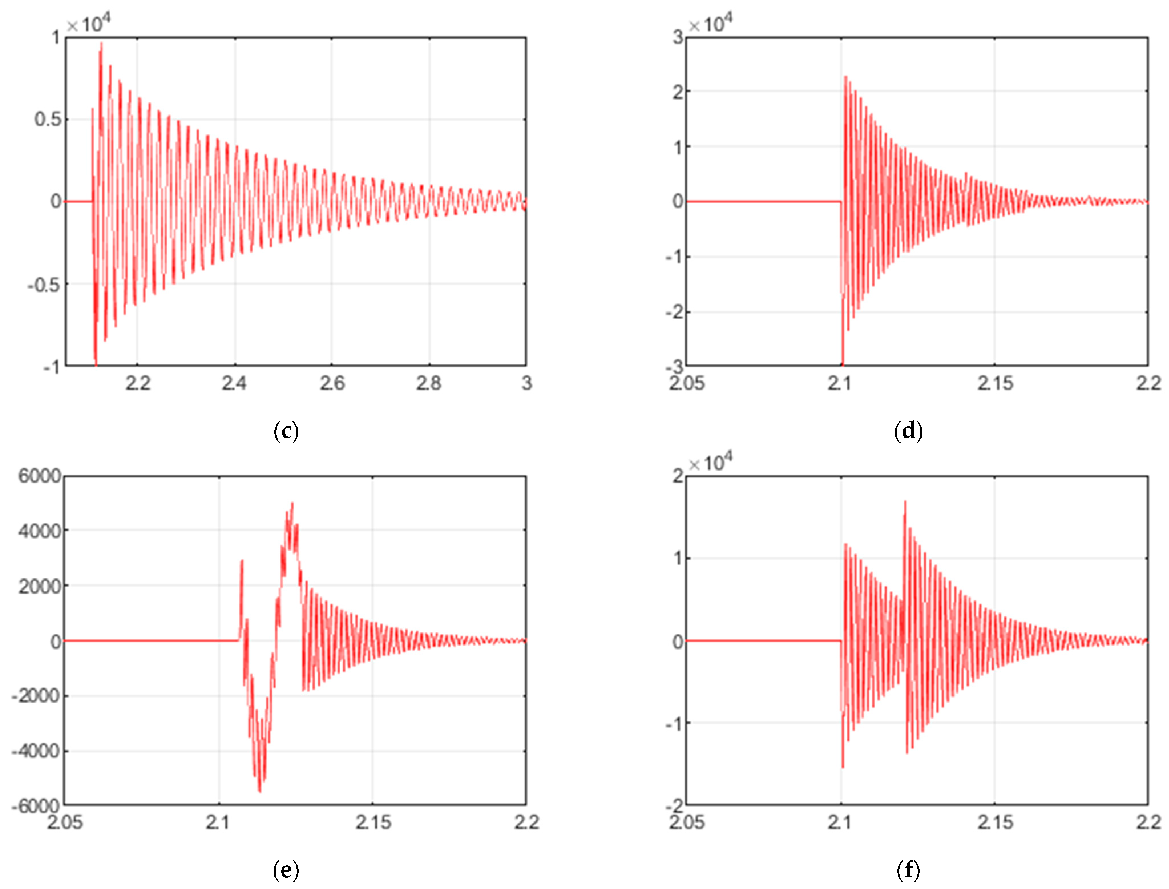
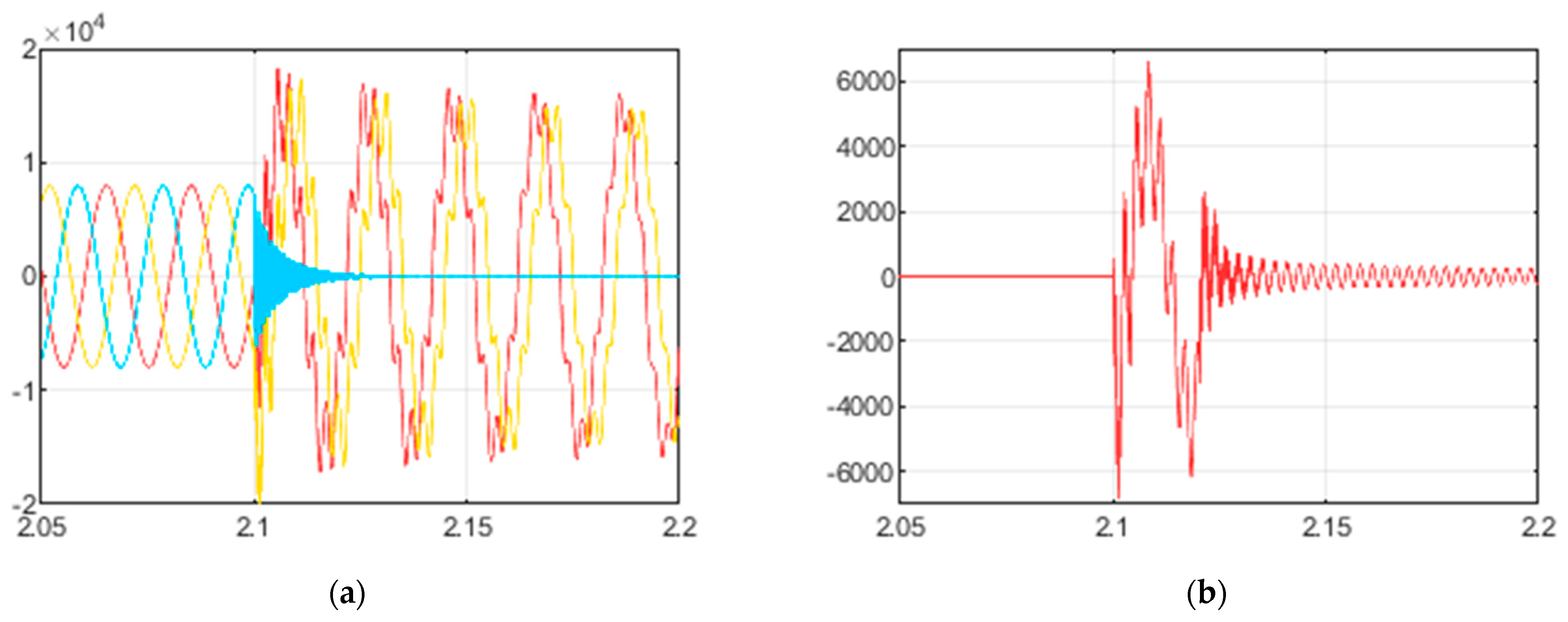
2.1.2. Atmospheric Transients

The second type to be investigated is atmospheric transients. Various lightning models are proposed in the literature; for example, one of the most popular is the Heidler function:

$$I\left(t\right)=\frac{I_m}{k}·\frac{{\left(\frac{t}{{\tau }_1}\right)}^n}{1+{\left(\frac{t}{{\tau }_1}\right)}^n}·\exp \left(-\frac{t}{{\tau }_2}\right),$$

(6)

where $I_m$—current peak value; $k$—correction factor of current peak value; $n$—steepness factor (equal to 10 according to IEC 62305-1:2010 [43], but other values can also be found in the scientific literature); ${\tau }_1$—rise time constant; ${\tau }_2$—fall time constant [43,44,45].

Another example can be obtained from [46]:

$$I\left(t\right)=I_m\left(\exp \left(-C_{1}t\right)-\exp \left(-C_{2}t\right)\right),$$

(7)

where $I_m$—current peak value; $C_1$ and $C_2$—constants.

According to IEEE Std 998-2012 [47], the average peak current of the first negative return stroke is 15–20 kA. The positive strokes’ current is typically higher, and its preferred limit for lightning protection is 200 kA. In nature, a 200 kA stroke occurs rarely—approximately 1% of all cases [42,47]. The selection of both the model and its parameters depends on the purpose: for example, for lightning protection design, parameters are selected with a margin. The goal of this paper is to model the situation as realistically as possible. The following function for lightning impulse modeling is selected:

$$I\left(t\right)=\{\begin{array}{ll}0,\hfill & t\in (-\infty ;T_0]\hfill \\ I_m\left(1-\exp \left(-\frac{t}{t_1}\right)\right),\hfill & t\in (T_0;T_1]\hfill \\ I_m\left(\exp \left(-\frac{t}{t_2}\right)-\exp \left(-\frac{t}{t_1}\right)\right),\hfill & t\in \left(T_1;+\infty \right)\hfill \end{array}$$

(8)

where $I_m$—current peak value; $t_1$—rise time; $t_2$—fall time; $T_0$—moment of the beginning; $T_1$—moment of the peak.

When $I\left(t\right)$ is known, the electric charge of the stroke is determined by:

$$Q=\underset{0}{\overset{\infty }{{\displaystyle \int }}}Idt.$$

(9)

The following information about the interconnection between the lightning stroke current $I\left(t\right)$ and induced voltage is important for modeling adequacy estimation. A direct lightning strike may raise voltage up to 1000 kV, and several hundred kilovolts may be induced when the distance from the power line is greater than 5 km [42]. For better intuition, the following results, found in the literature, are given as an example:

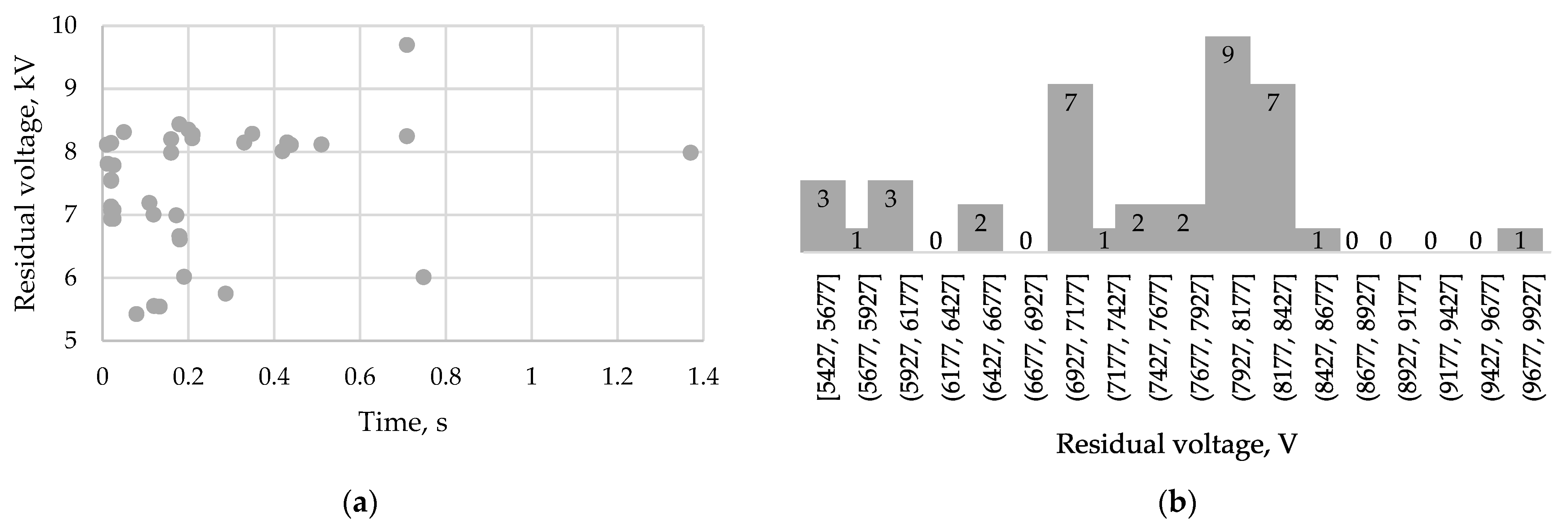
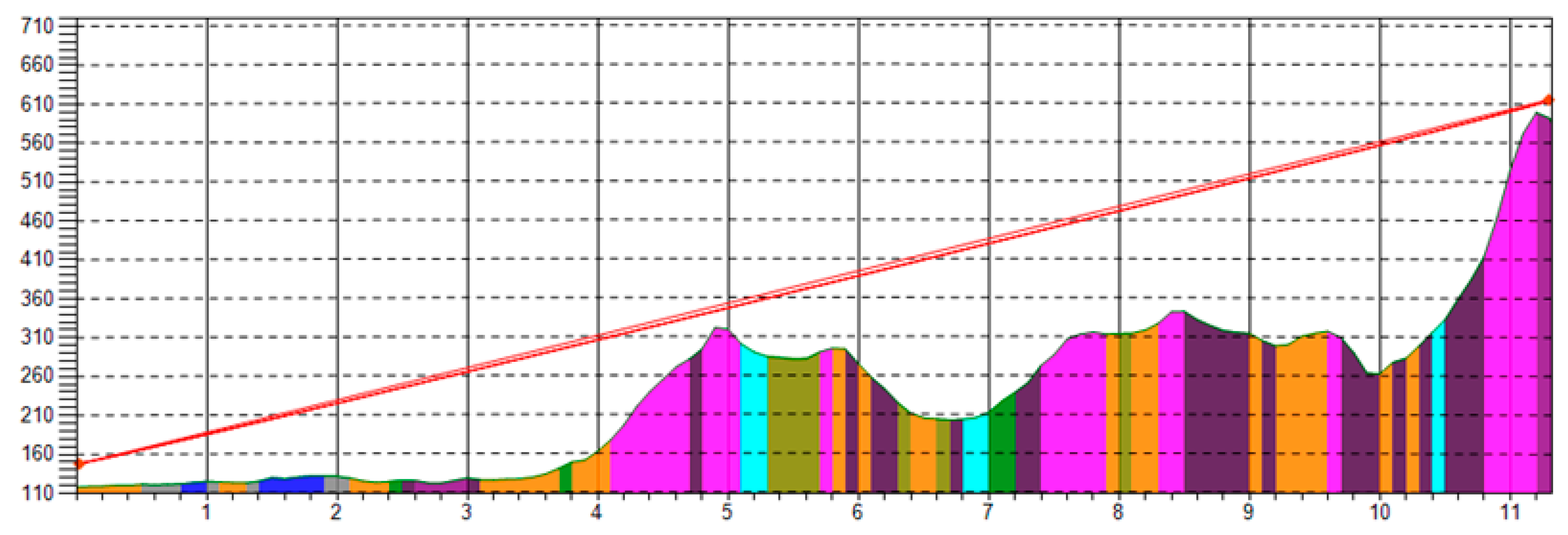
• According to the calculations given in [42] (pp. 268–269), when the striking distance was 30 m, a 30 kA impulse induced an approximately 195 kV voltage peak, when 100 m—approximately 50 kV, and when 300 m—approximately 20 kV. The duration of these impulses is longer than 6 μs (see Section 4.1 for more details and discussion about the duration of transients). It was assumed that the height of the line (above ground) is 5 m (this assumption is not realistic), the steepness of the impulse is 20 kA/μs (see Equation (10)), the rise time of the impulse is 1.5 μs, and the speed of the return stroke is equal to 0.1 of the speed of light.
• In [45], when the striking distance was 1.16 m, 10 kA impulse induced 50 kV voltage, but the predicted result from theoretical simulation was 28 kV. The length of the single-phase overhead power line is 200 m, and the height is 10 m. The durations of induced impulses are up to 10–20 μs.
• In [46], when the striking distance was 50 m, the 12 kA impulse induced 52–80 kV voltages at various points of the single-phase overhead power line whose length is 1 km and height is 10 m. The duration of the induced impulse is up to 10 μs.

It is noteworthy that the induced overvoltage depends on lightning impulse steepness, which is defined as:

$$\alpha =\frac{dI}{dt}.$$

(10)

This is due to Faraday’s law of induction:

$$\nabla \times E=-\frac{\partial B}{\partial t} \iff {{\displaystyle \oint }}_l^{}E·dl=-{{\displaystyle \int }}_S^{}\frac{\partial }{\partial t}B·dS,$$

(11)

where $E\left(r,t\right)$—electric field (generally, a function of position $r$ and time $t$); $B\left(r,t\right)$—magnetic field; $dl$—infinitesimal vector element of the contour; $dS$—infinitesimal vector element of the surface; $\nabla$—del operator.

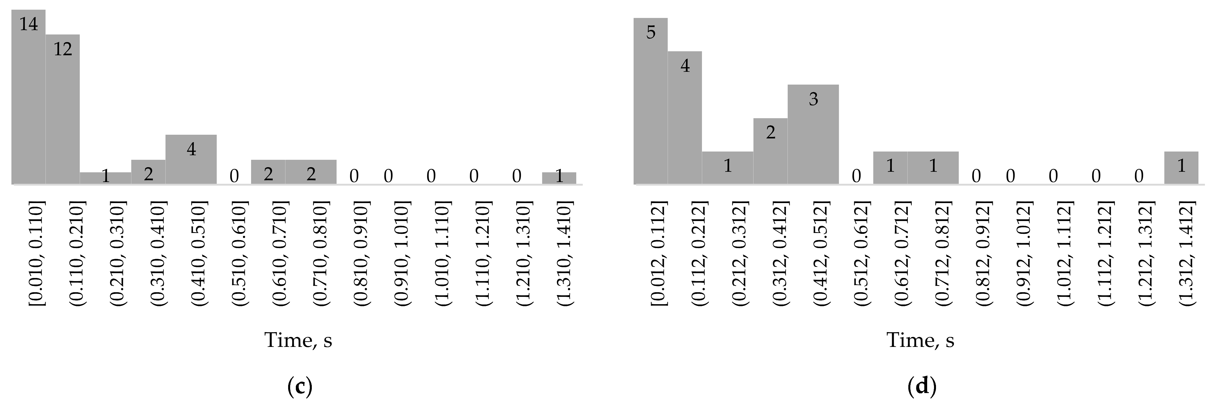
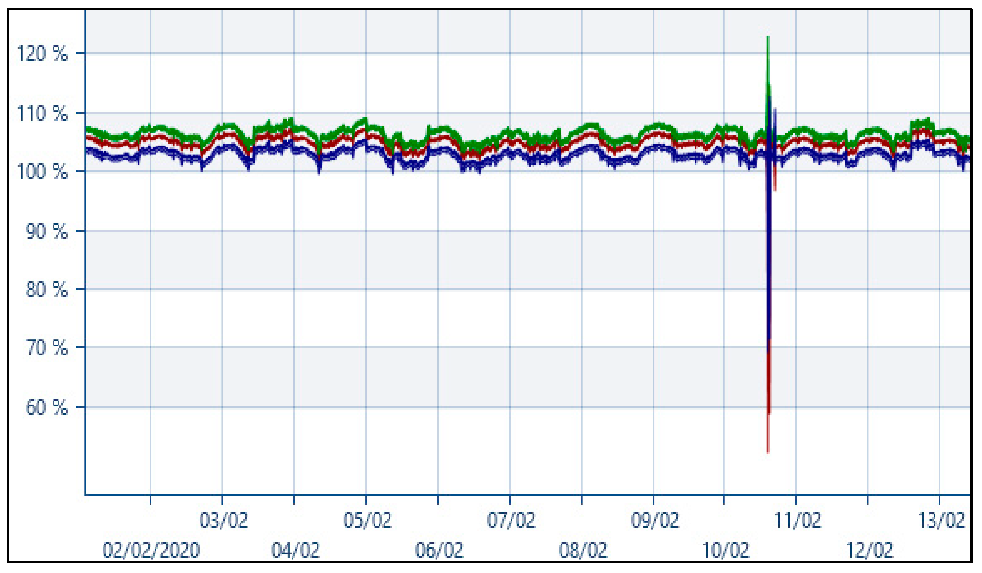
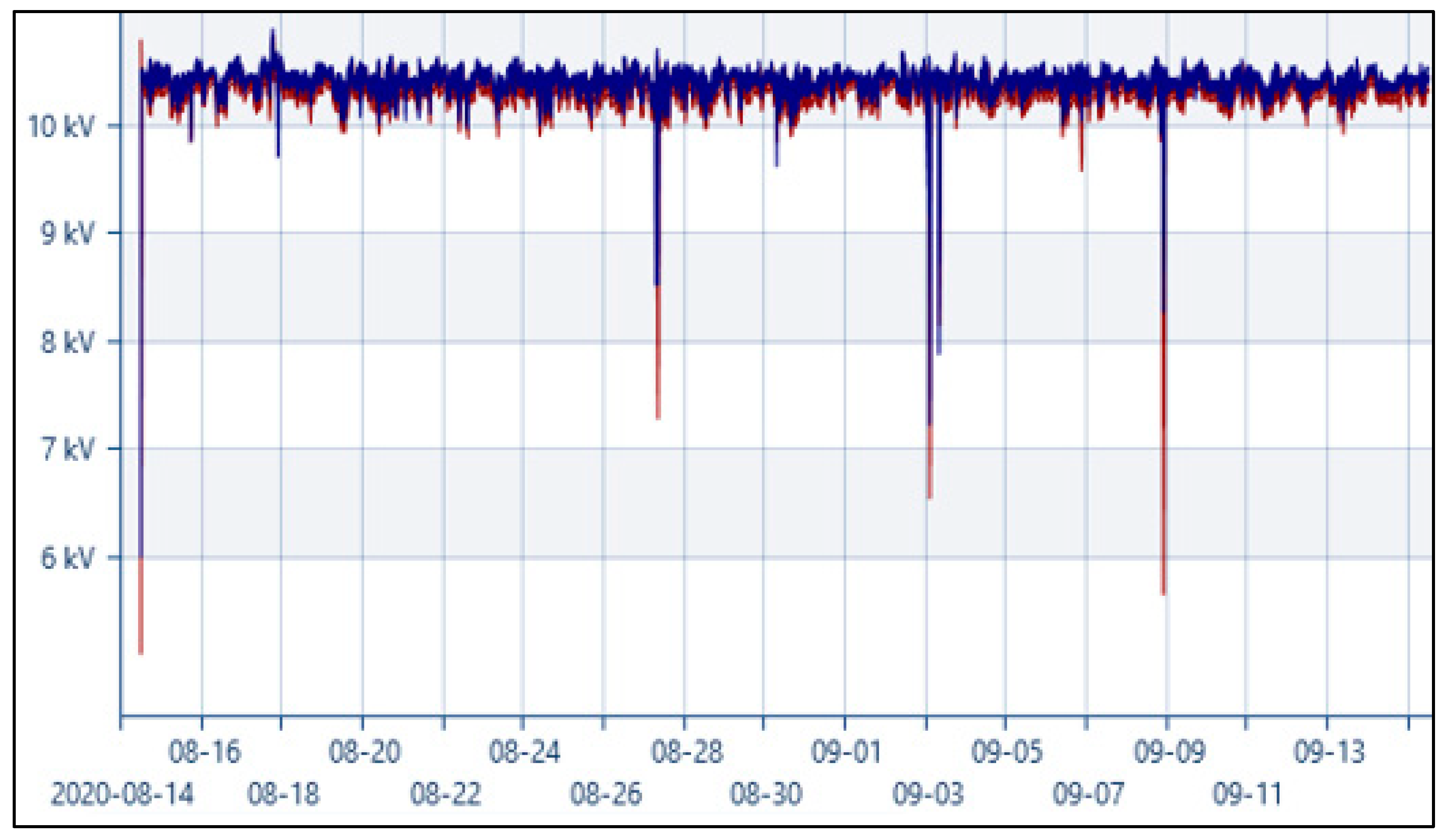
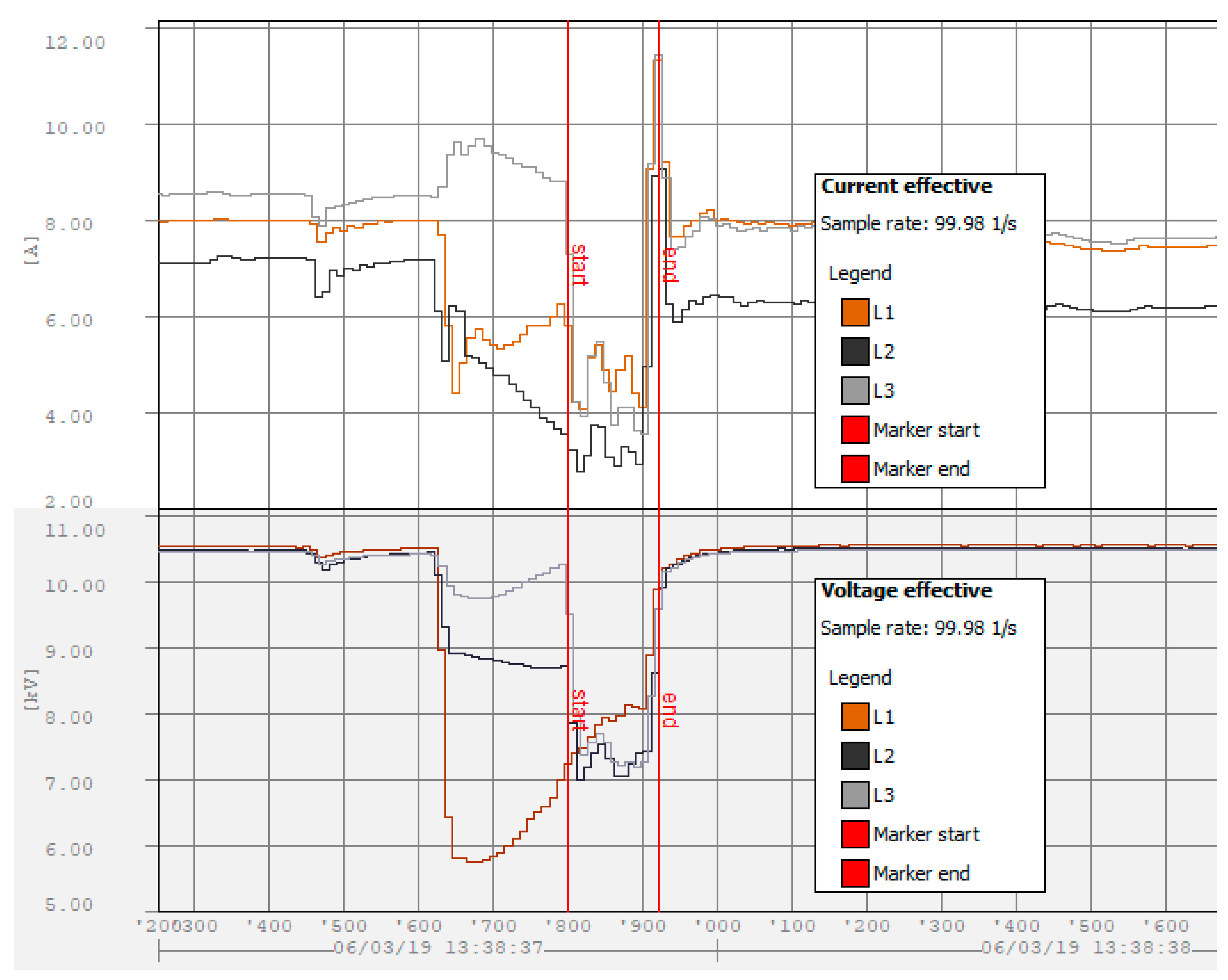
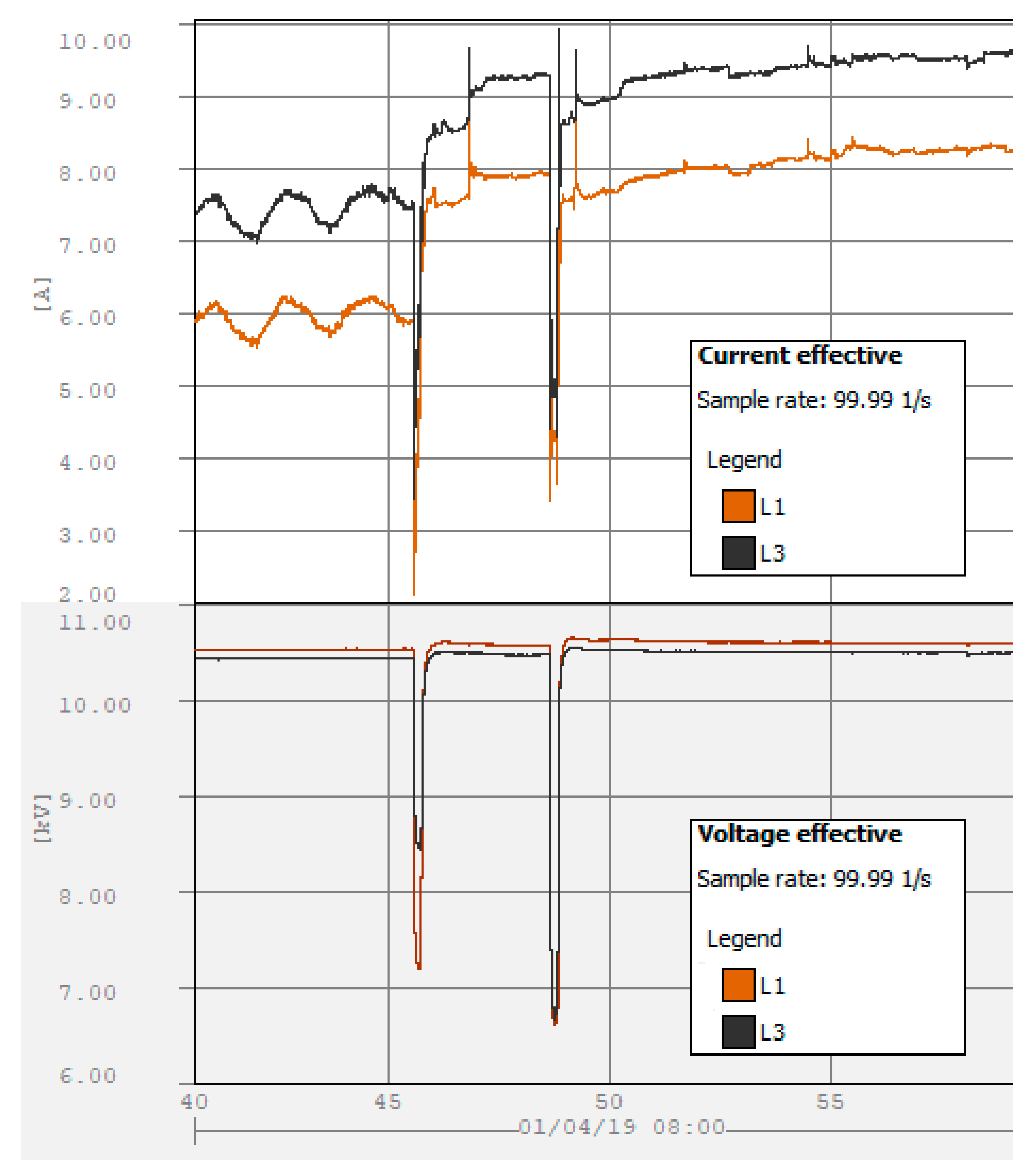
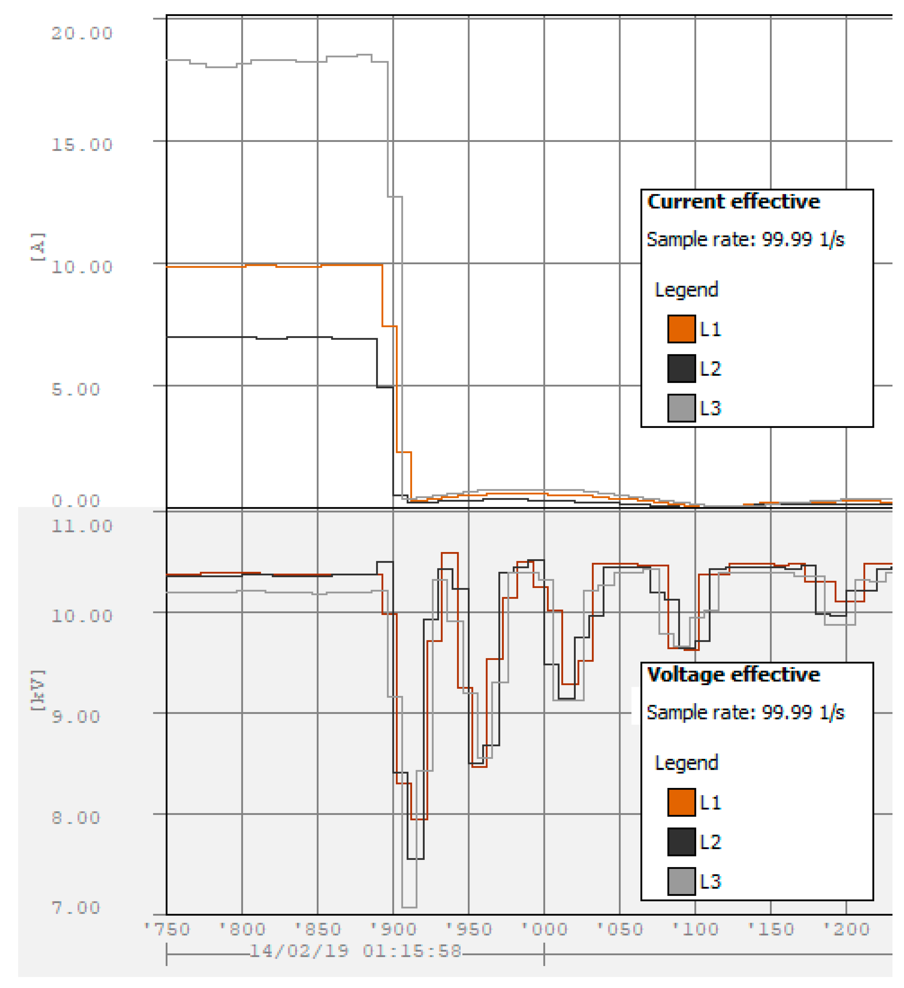
2.1.3. Short-Duration RMS Variations: PQ Monitoring Campaign

IEEE Std 1159-2019 classifies RMS variations by time into two categories—short duration (shorter than 1 min) and long duration (longer than 1 min). EN 50160:2010 limits the duration up to 1 min in all recommended tables for voltage sags and swells classification. The duration of short-duration RMS events highly depends on the settings of relay protection and automation. In our opinion, RMS variations which last longer than 1 min can be excluded from the target group of this paper. The data were obtained from the measurement campaigns and theoretical simulations. Since the theoretical research of short circuits is described in detail in [9] (with the intention to be used as a database), let us continue with the PQ monitoring campaign in the Lithuanian DSO grid. The main focus of the campaign was on voltage sags; however, we have discovered that accurate calculation of the total number of events is a complicated task. Honestly, since data gathering and processing have been mainly manual to date, a tribute must be paid to those authors who at least roughly succeeded in the implementation of this (e.g., see the practical researches listed in [2]). On the other hand, in our opinion, such statistics are not important for this research, but we will present a few episodes. An absolute majority of the recorded sags were caused by grid faults; however, since the main focus was on the power supply of industrial plants, there is a small probability that at least few of them were caused by electric motor starting. The latest voltage sag in possession was recorded at the 0.4 kV point of common coupling of medical equipment manufacturer (in Kaunas municipality): the three-phase phase-to-ground voltage dropped from 230–240 V to 170–222 V (the sag’s duration was 0.34 s).

In Figure 2, the statistics of the 35/10 kV substation (in Širvintos municipality) are given when a PQ analyzer was installed on the 10 kV side from January to April 2019. In the first three charts, voltage arrays are analyzed separately, i.e., the multiphase aggregation which is required in EN 50160:2010 is not applied. Such an approach will often be preferred in this work (see Section 4.1 for the argumentation). It can be noticed that the data are distributed randomly and do not follow any distribution. A trend appearance may be expected with an increase in observation period (according to the law of large numbers); however, 2–3 years may not be enough for that: the minimum monitoring period for voltage sags, swells and interruptions, recommended by IEC 61000-4-30:2015, is 1 year. Also, it should be noted that 50% and deeper sags have not occurred, which means the absence of critical situations. The shortest recorded sag duration is 0.010 s (Figure 2c), which matches the smallest possible time window defined by IEC 61000-4-30. After the multiphase aggregation, the minimal duration becomes 0.012 s (Figure 2d). The bin width of the voltage histogram is 300 V (Figure 2b), and the bin width of time histograms is 0.100 s (Figure 2c,d). The sample size of phase-to-phase voltage AB (i.e., voltage between phase A and phase B) is 11, BC—17, CA—11 (i.e., a total of 39); the means of durations—0.33 s, 0.25 s, and 0.17 s; the medians of durations—0.13 s, 0.18 s, and 0.16 s; the means of residual voltages—7383 V, 7571 V, and 7956 V; the medians of residual voltage—7789 V, 8011 V, and 7136 V (respectively).

To continue, phase-to-ground voltage measurements in the 35 kV line (located in Rokiškis municipality) taken from 1 February 2020 to 13 February 2020 are given in Figure 3, and those taken from 15 August 2020 to 14 September 2020 are given in Figure 4. As in the previous case, there have been no sags deeper than 50%. In spite of EN 50160:2010 requirement to assess phase-to-phase voltage, phase-to-ground voltage arrays are more informative due to at least a single-phase fault identification possibility. Also, in Figure 4, the scattering of voltage phasors is given: phase unbalance can be caused by an asymmetrical fault (see [9] for examples). It is noteworthy that not every software is able to display the voltage of entire measurement period in one window (as shown in the figures); however, such a functionality is not essential for this research.

Phase-to-ground voltage measurements in the 10 kV line (located in Rokiškis municipality) taken from 15 August 2020 to 15 September 2020 are given in Figure 5. Only two (of three) arrays are available due to the absence of one phase-to-ground voltage transformer. In the case of asymmetrical faults, the PQ analyzer assumes that the mode is symmetrical; thus, the estimation of the unknown voltages will be incorrect (inaccurate).

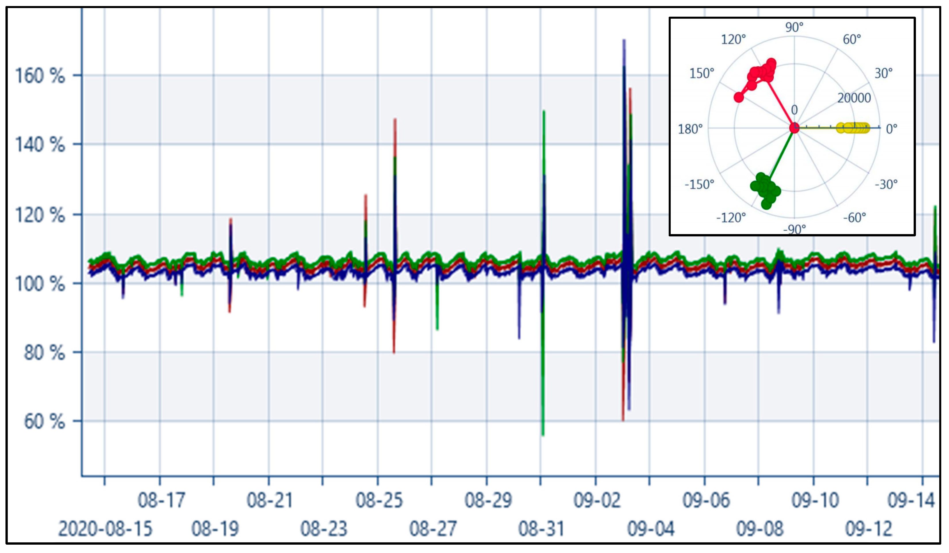
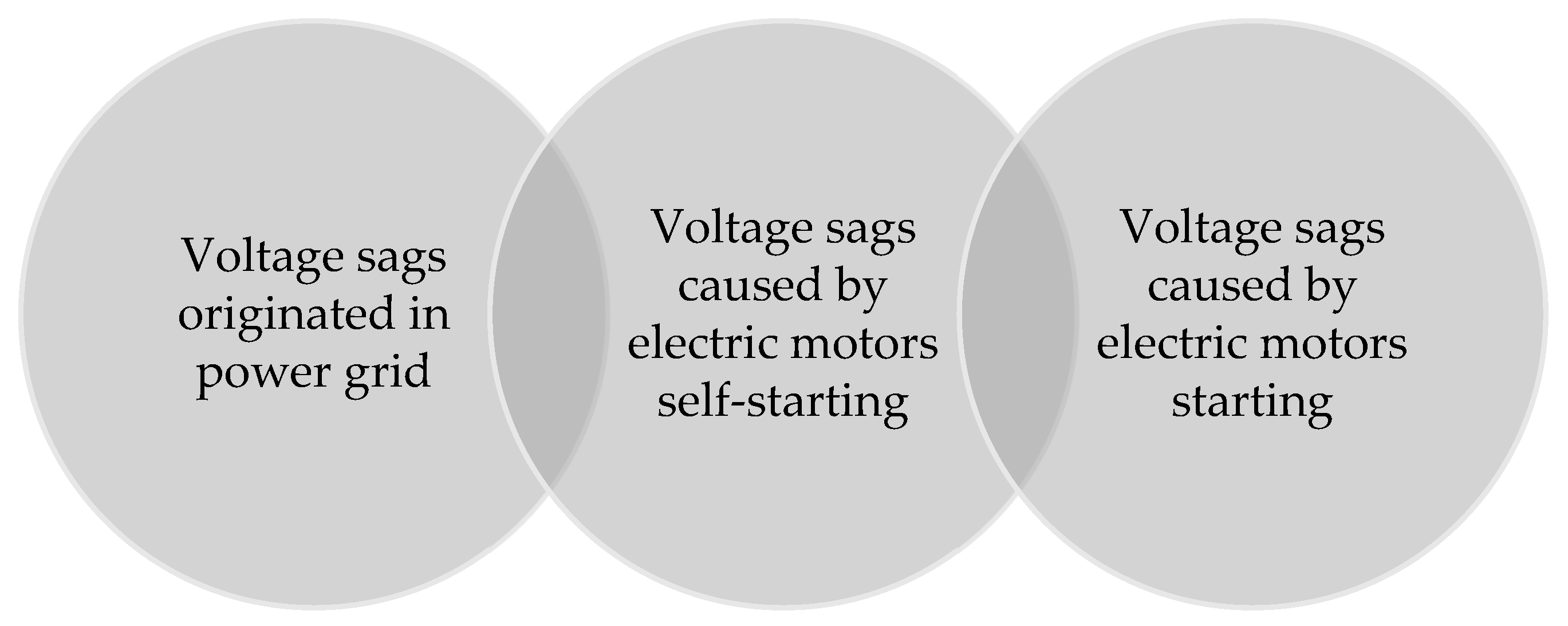
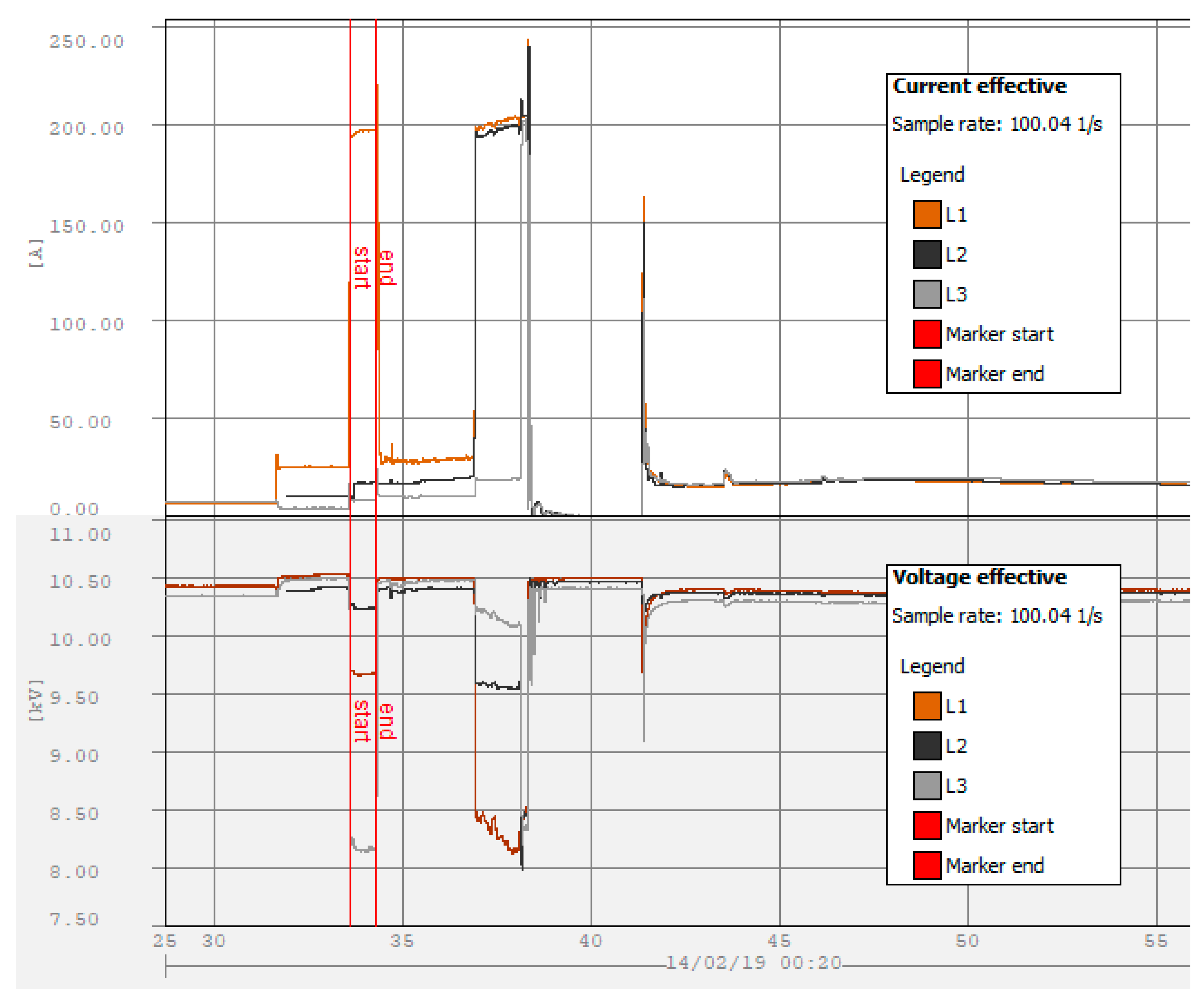
2.1.4. Voltage Sags Caused by Electric Motor Starting

Another cause of voltage sag, which we would like to include, is the electric motor starting. At first glance, it seems that the data can be obtained from both practical experiments and simulations. However, the prerequisites of such an experimental work are not only the special set-up but also many different motors are required to be in possession. The simulation of an electric motor behavior requires impedance data of equivalent circuit as well as some other parameters such as rotational speed and mechanical inertia (e.g., see [48,49] for the case of a squirrel-cage induction motor). In this context, similarly as in the case of atmospheric transients (Section 2.1.2), it was decided that the most efficient way to become familiar with the topic and obtain the initial information is a literature review, postponing a more detailed investigation for the future. The following results can be given as an example:

• One figure is given in IEEE Std 1159-2019 (p. 22): the minimal residual voltage is 0.8 p.u., and the voltage sag duration is approximately 2 s. The motor type is not specified, but it is mentioned that a motor is large.
• In [14] that investigates an induction motor fed by a current controlled pulse width modulation inverter, the minimal residual voltage and duration of the simulated voltage sag is 0.88 p.u. and 0.8 s.
• In [49] (investigates an induction squirrel-cage motor), the minimal residual voltage and duration of voltage sags are as follows: (1) 0.35 p.u. and 307 ms (simulated) or 327 ms (measured) with the capacitor bank switching; (2) 0.25 p.u. and 710 ms without the capacitor bank switching. The simulation results coincide with the experimental results. It should be noticed that the applied AC motor starting method (as well as others, for example, reactor starting, autotransformer starting, Y-Δ transform, etc.) limits both inrush current and voltage sag.
• In [50] that investigates water pumps driven by the induction motors, the minimal residual voltage and duration of both simulated voltage sags are 0.85–0.87 p.u. and 0.05 s.

Please note that the given results reflect the influence of only one electric motor. In the case of a three-phase electric motor, the voltage sag is symmetrical.

To continue, in our previous work [9], similarly but not analogously to [48], the opposite case—effect of symmetrical voltage sags on electric motors—is investigated. The intermediate chain between both cases is the sags caused by a motor self-starting (see Figure 6). The higher generation of an electric motor is during a grid fault, the higher and longer-lasting is the residual voltage, and the higher is the probability of self-starting (which again reduces the voltage, thereby lowering the probability of own success) [51]. In practice, industrial companies can prioritize the self-starting of their motors; however, due to limited time, the prioritization cannot solve all problems and fully prevent the stoppages. Despite electrical machine engineering being a mature scientific field, there is still a lack of information on the topic, in particular through a prism of PQ.

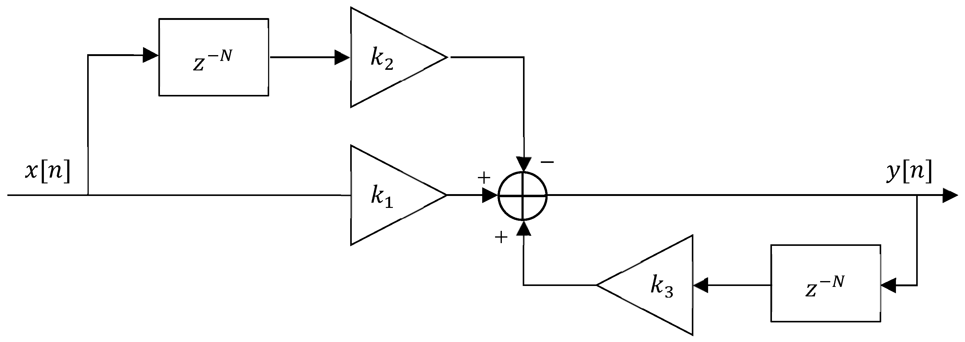
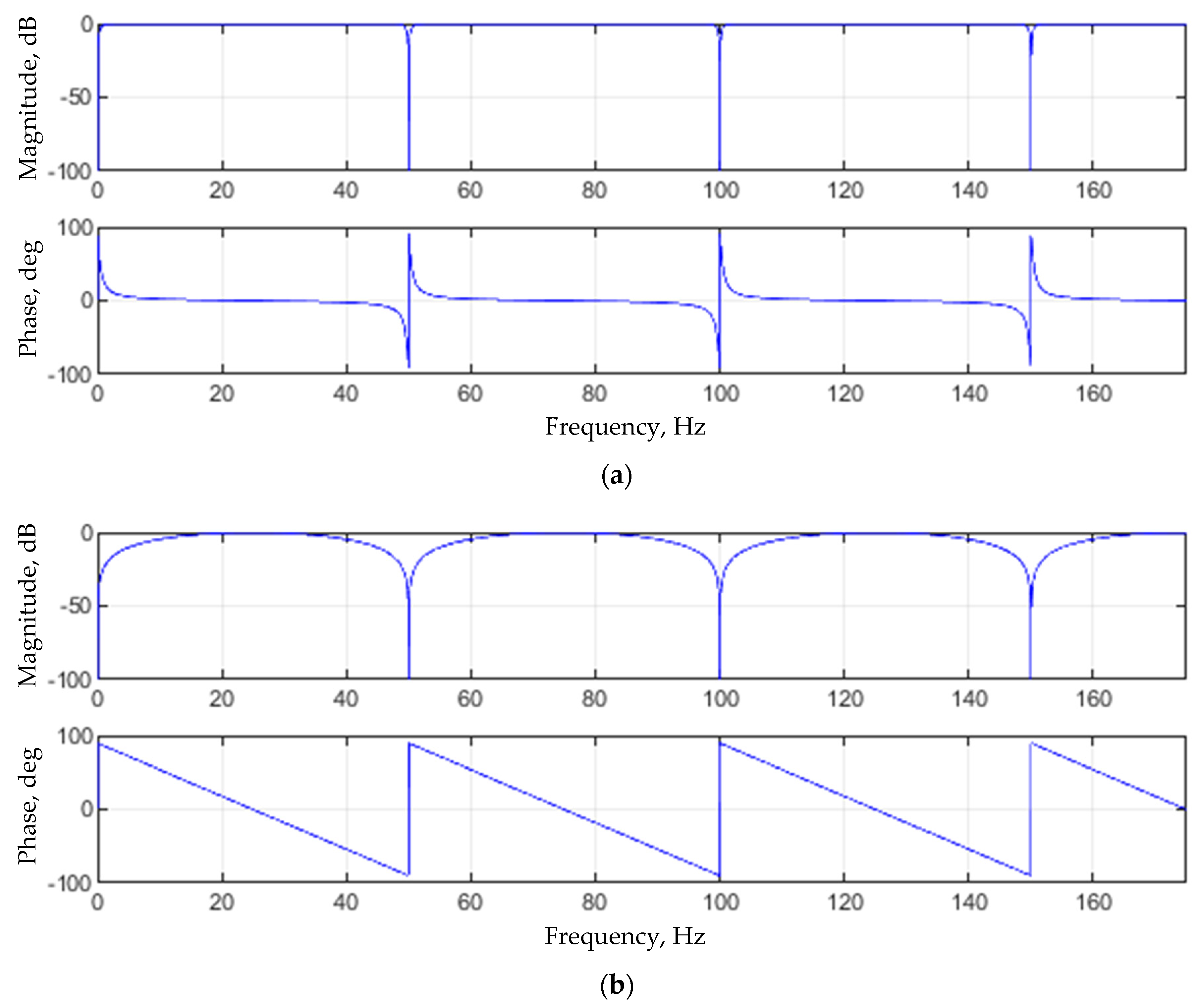
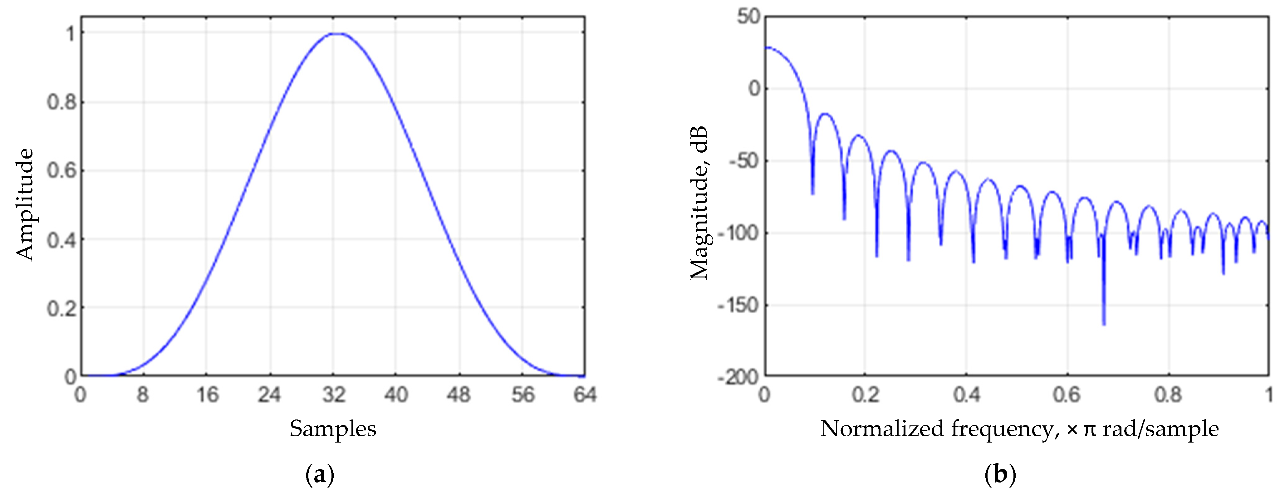
2.2. Shelving Filter

As has been mentioned previously, both impulsive and oscillatory transients can be analyzed (measured) with or without the fundamental frequency component included [12]. Inspired by [52], the application of an infinite impulse response (IIR) shelving filter, obtained from [53], will be investigated for 50 Hz component removal from a PQ signal. The block diagram of the filter is given in Figure 7. It is noteworthy that any application of this filter for a PQ signal has not been found in the literature.

In Figure 7, it can be noticed that the implementation of the filter requires three operations of summation and three operations of multiplication. The filter has three coefficients $k_1$, $k_2$ and $k_3$, and its difference equation is:

$$y\left[n\right]=k_{1}x\left[n\right]-k_{2}x\left[n-N\right]+k_{3}y\left[n-N\right],$$

(12)

where $x\left[n\right]$—input; $y\left[n\right]$—output; $n$—sample number; $N$—delay.

The transfer function of the filter is:

$$H\left(z\right)=\frac{Y\left(z\right)}{X\left(z\right)}=\frac{k_1-k_2{z}^{-N}}{1-k_3{z}^{-N}},$$

(13)

where $X\left(z\right)$—Z-transform of $x\left[n\right]$; $Y\left(z\right)$—Z-transform of $y\left[n\right]$.

It is noteworthy that the Z-transform of a discrete-time signal $x\left[n\right]$ is defined as follows:

$$X\left(z\right)=\mathcal{Z}\left\{x\left[n\right]\right\}={\displaystyle \sum }_{-\infty }^{\infty }x\left[n\right]z^{-n},$$

(14)

where $n$ is an integer, and $z$ is, in general, a complex number which may be written in polar form:

$$z=r{e}^{j\varphi }=r\left(\cos \varphi +j\sin \varphi \right).$$

(15)

where $r$—magnitude; $\varphi$—complex argument; $j$—imaginary unit.

Coefficients $k_1$, $k_2$ and $k_3$ are calculated as follows:

$$k_1=\frac{K_0+K\beta }{1+\beta },$$

(16)

$$k_2=\frac{K_0-K\beta }{1+\beta },$$

(17)

$$k_3=\frac{1-\beta }{1+\beta }.$$

(18)

Parameter $\beta$ is calculated by:

$$\beta =\frac{K_r{}^2-K_0{}^2}{K^2+K_r{}^2}\tan \left(\frac{\pi ·N·\Delta f}{2f_s}\right),$$

(19)

where $K_0$—gain of passband; $K$—attenuation of stopband; $N$—number of cuts; $\Delta f$—stopband width at $K_r$ level, Hz; $f_s$—sampling frequency, Hz.

The number of cuts $N$ is determined as follows:

$$N=\frac{f_s}{f_0},$$

(20)

where $f_0$—frequency to be filtered and its harmonics, Hz.

Parameters $K$ and $K_r$ are calculated by:

$$K=K_0·{10}^{-\frac{A}{20}},$$

(21)

$$K_r=K_0·{10}^{-\frac{L}{20}},$$

(22)

where $A$—attenuation, dB; $L$—level of the cutoff frequency, dB.

2.3. Fundamental Theory of SVM

SVM is a supervised learning algorithm used for classification and regression as well as outlier detection. A large amount of information about it can be found in various literature, for example, in [7,54,55,56]. SVM by its origin is a binary classification algorithm, but it can be extended to any multiclass case by combining the binary classifiers using either the one-versus-one or one-versus-rest approach.

Consider the training sample:

$$\mathcal{T}=\left\{\left(x_1,y_1\right),\left(x_2,y_2\right),\dots ,\left(x_n,y_n\right)\right\},$$

(23)

where $x_i$—multi-dimensional real vector; $y_i$—class label of $x_i$. The goal of SVM is to construct a decision boundary separating the feature vectors $x_i$ into two groups whose labels are either $y_i=1$ or $y_i=-1$ in the way that ensures that the total distance between the decision boundary and the nearest points from both groups is maximized. In linear cases, the equation of a decision surface in the form of a hyperplane is as follows:

$$w^{\mathrm{T}}x+b=0,$$

(24)

where $w$—adjustable (and not necessarily normalized) normal vector to the hyperplane (also called the weight vector); $x$—input vector; $b$—bias. The parameter $\frac{b}{\Vert w\Vert }$ determines the offset of the hyperplane from its initial position along the vector $w$. Therefore, the Euclidian norm $\Vert w\Vert$ needs to be minimized in order to maximize the margin of separation. In the case of a hard margin, the principle of SVM linear separation takes the following form:

$$\{\begin{array}{ll} w^{\mathrm{T}}{x}_i+b\ge 1,\hfill & \mathrm{if} y_i=1\hfill \\ w^{\mathrm{T}}{x}_i+b\le -1,\hfill & \mathrm{if} y_i=-1\hfill \end{array}\Rightarrow y_i\left(w^{\mathrm{T}}{x}_i+b\right)\ge 1,\forall i\in \left\{1, 2,\dots ,n\right\}.$$

(25)

In case of overlapping data, when a line cannot separate groups without any mistake, SVM classification is extended by establishing the soft margin concept. It allows misclassification to happen, thereby violating the condition of Equation (25) and raising the need to minimize classification error $\xi$. Thus, Equation (25) becomes:

$$y_i\left(w^{\mathrm{T}}{x}_i+b\right)\ge 1-{\xi }_i, {\xi }_i\ge 0, \forall i\in \left\{1, 2,\dots ,n\right\},$$

(26)

where ${\xi }_i$—slack variable, which is a measure of the deviation from the ideal points separation. If ${\xi }_i>1$, the point falls on the wrong side of the margin. The goal of optimization is based on the hinge loss, which is a loss function used in training classifiers (in particular SVM). Let us skip the intermediate steps with the hinge loss (since they are beyond the scope of this paper) and give the final formulation of the optimization problem:

$$\min \left(\frac{1}{2}{\Vert w\Vert }^2+C{\displaystyle \sum }_{i=1}^N{\xi }_i\right),$$

(27)

where $C$—regularization parameter. The parameter $C$ controls the width of the gap (margin size) in exchange of misclassification, and it has to be set by the user. Larger values of $C$ correspond to the harder margin.

Nonlinear classification can also be efficiently performed with SVM. Two nonlinear kernels are used in this paper. The radial basis function (RBF) kernel is defined as follows:

$$k\left(x_j,x_k\right)=\exp \left(-\frac{\Vert x_j-x_k\Vert {}^2}{2{\sigma }^2}\right),$$

(28)

where $\Vert x_j-x_k\Vert {}^2$—squared Euclidian distance between the two feature vectors; $\sigma$—width, which is often expressed as:

$$\gamma =\frac{1}{2{\sigma }^2}.$$

(29)

The polynomial kernel function takes the following form:

$$k\left(x_j,x_k\right)={\left(x_j{}^{\mathrm{T}}{x}_k+c\right)}^p,$$

(30)

where $c$—non-negative free parameter; $p$—degree of the polynomial.

It is noteworthy that $k\left(x_j,x_k\right)=k\left(x_k,x_j\right)$ (for both kernels explored), and the maximum value is reached when $x_j=x_k$ (but there is no such need of its existence) [54].

2.4. Fundamental Theory of KNN

KNN is a supervised learning algorithm which is also used for classification and regression. The main principle of label assignment is based on majority rule involving a selected number $k$ of nearest neighbors. This number is selected freely (but reasonably) by a user. Also, in a binary classification, it would be wise to choose an odd number since it allows avoiding tied votes [7]. Various methods can be used to estimate the distance (e.g., Chebyshev distance), but the already mentioned Euclidian distance, which is a special case of Minkowski distance, will be preferred in this paper. In n-dimensional space, the formula of Euclidian distance is:

$$d\left(p,q\right)=\Vert p-q\Vert =\sqrt{{\left(p_1-q_1\right)}^2+{\left(p_2-q_2\right)}^2+\dots +{\left(p_n-q_n\right)}^2},$$

(31)

where $p_i$ and $q_i$ are Cartesian coordinates of points $p$ and $q$ respectively.

One majority voting disadvantage occurs when the class distribution is skewed. This can be solved by the distance weighting. In this paper, the weights are inversely proportional to the distance, i.e., $1/d$. Therefore, closer points became more important than more distant ones. Also, it is noteworthy that KNN does not work well in high-dimensional spaces; this problem is called the curse of dimensionality, which is a phenomenon where feature space becomes increasingly sparse [7]. Intuitively, it can be understood that even the closest points can indeed be too distant in a high-dimensional space.

2.5. Additional Methods

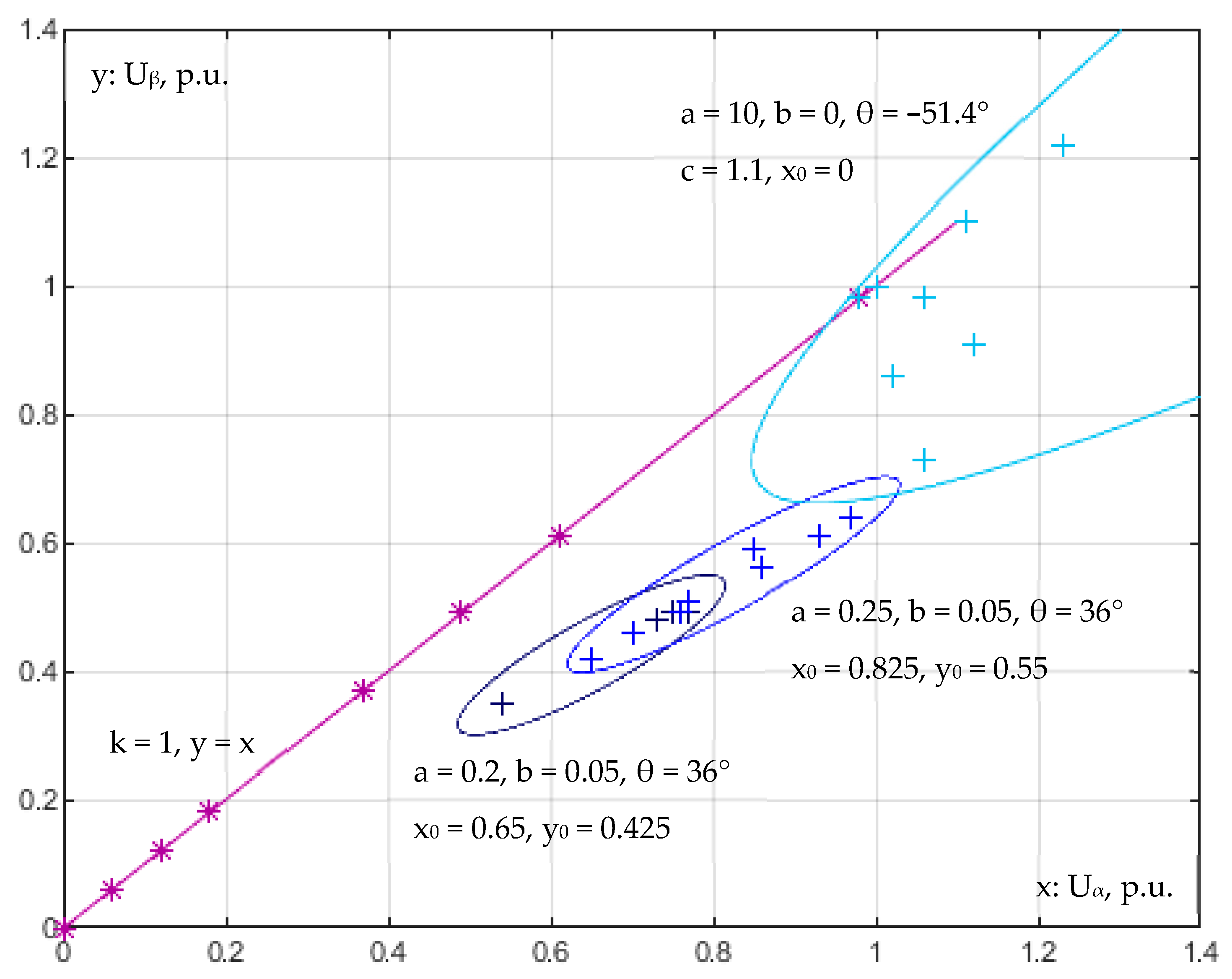
2.5.1. Geometric Analysis

In Section 3.2.2, data dispersion areas and their boundaries in the feature space are analyzed geometrically. For this purpose, in this section, a relevant theoretical background is given for both spaces ${ℝ}^2$ and ${ℝ}^3$.

When a line passes different points $\left(x_1,y_1,z_1\right)$ and $\left(x_2,y_2,z_2\right)$, the canonical equation of this line is as follows:

$$\frac{x-x_1}{x_2-x_1}=\frac{y-y_1}{y_2-y_1}=\frac{z-z_1}{z_2-z_1}.$$

(32)

The general equation of a plane is:

$$ax+by+cz+d=0,$$

(33)

where $a$, $b$ and $c$ are the components of the normal vector $n=\left\{a,b,c\right\}$ which is perpendicular to the plane.

The coplanarity condition of points $\left(x_1,y_1\right)$ and $\left(x_2,y_2\right)$ is given by:

$$\left|\begin{array}{ccc}x& y& 1\\ x_1& y_1& 1\\ x_2& y_2& 1\end{array}\right|=0.$$

(34)

The canonical equation of an ellipsoid is:

$$\frac{{\left(x-x_0\right)}^2}{a^2}+\frac{{\left(y-y_0\right)}^2}{b^2}+\frac{{\left(z-z_0\right)}^2}{c^2}=1,$$

(35)

where $\left(x_0,y_0,z_0\right)$—center coordinates; $a$, $b$ and $c$—the lengths of the semi-axes. In a two-dimensional case, when $z=0$, then Equation (35) represents an ellipse.

An elliptic paraboloid is represented by the following equation:

$$z=\frac{{\left(x-x_0\right)}^2}{a^2}+\frac{{\left(y-y_0\right)}^2}{b^2}+z_0,$$

(36)

where $\left(x_0,y_0,z_0\right)$—center coordinates; $a$ and $b$—constants.

The equation of a parabola, whose vertex coordinates are $\left(x_0,c\right)$, is given by a univariate quadratic function:

$$a{\left(x-x_0\right)}^2+b\left(x-x_0\right)+c=0.$$

(37)

Rotation in two-dimensional Euclidian space is performed with the rotation matrix:

$$R=\left[\begin{array}{cc}\cos \theta & -\sin \theta \\ \sin \theta & \cos \theta \end{array}\right],$$

(38)

where $\theta$—rotation angle about the origin of a two-dimensional Cartesian coordinate system. The positive angle corresponds to a counterclockwise rotation, and negative corresponds to a clockwise rotation. In the case of three-dimensional Euclidian space, the rotation matrix takes the following form:

$$R=\left[\begin{array}{ccc}\cos \alpha & -\sin \alpha & 0\\ \sin \alpha & \cos \alpha & 0\\ 0& 0& 1\end{array}\right]\left[\begin{array}{ccc}\cos \beta & 0& \sin \beta \\ 0& 1& 0\\ -\sin \beta & 0& \cos \beta \end{array}\right]\left[\begin{array}{ccc}1& 0& 0\\ 0& \cos \gamma & -\sin \gamma \\ 0& \cos \gamma & \cos \gamma \end{array}\right],$$

(39)

where $\alpha$, $\beta$ and $\gamma$ are Euler angles about the abscissa, ordinate and applicate, respectively.

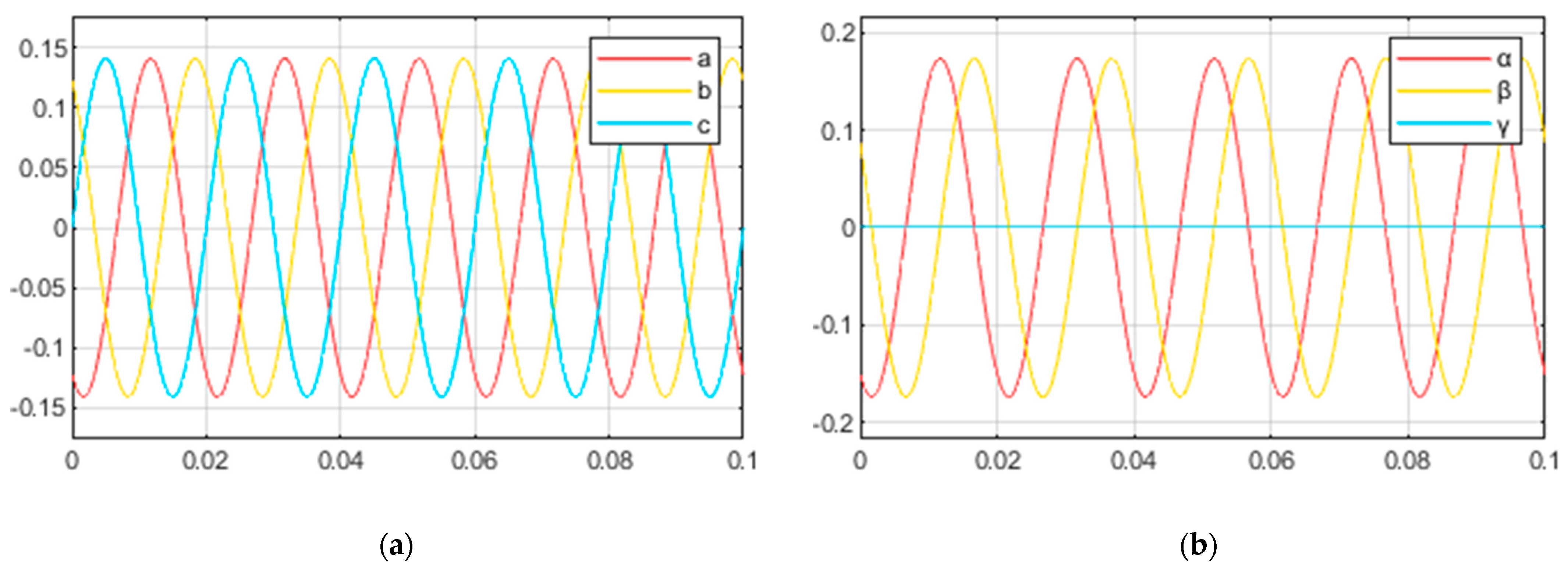
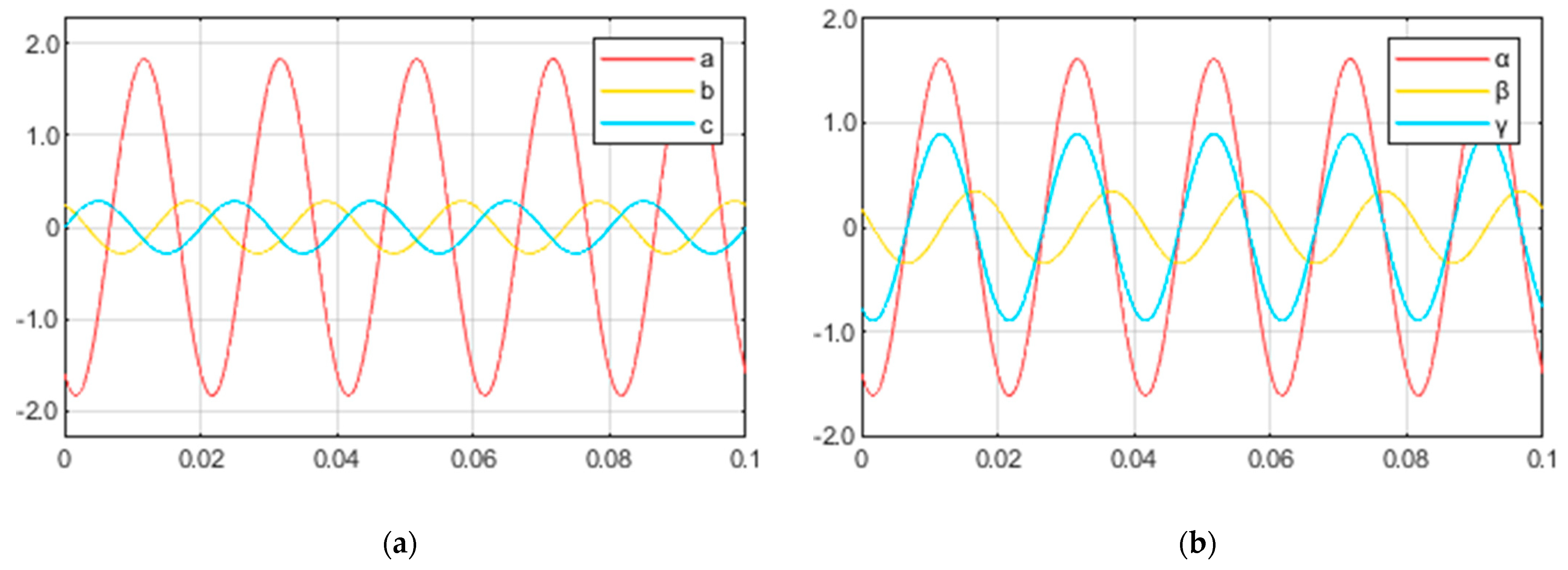
2.5.2. Clarke Transformation

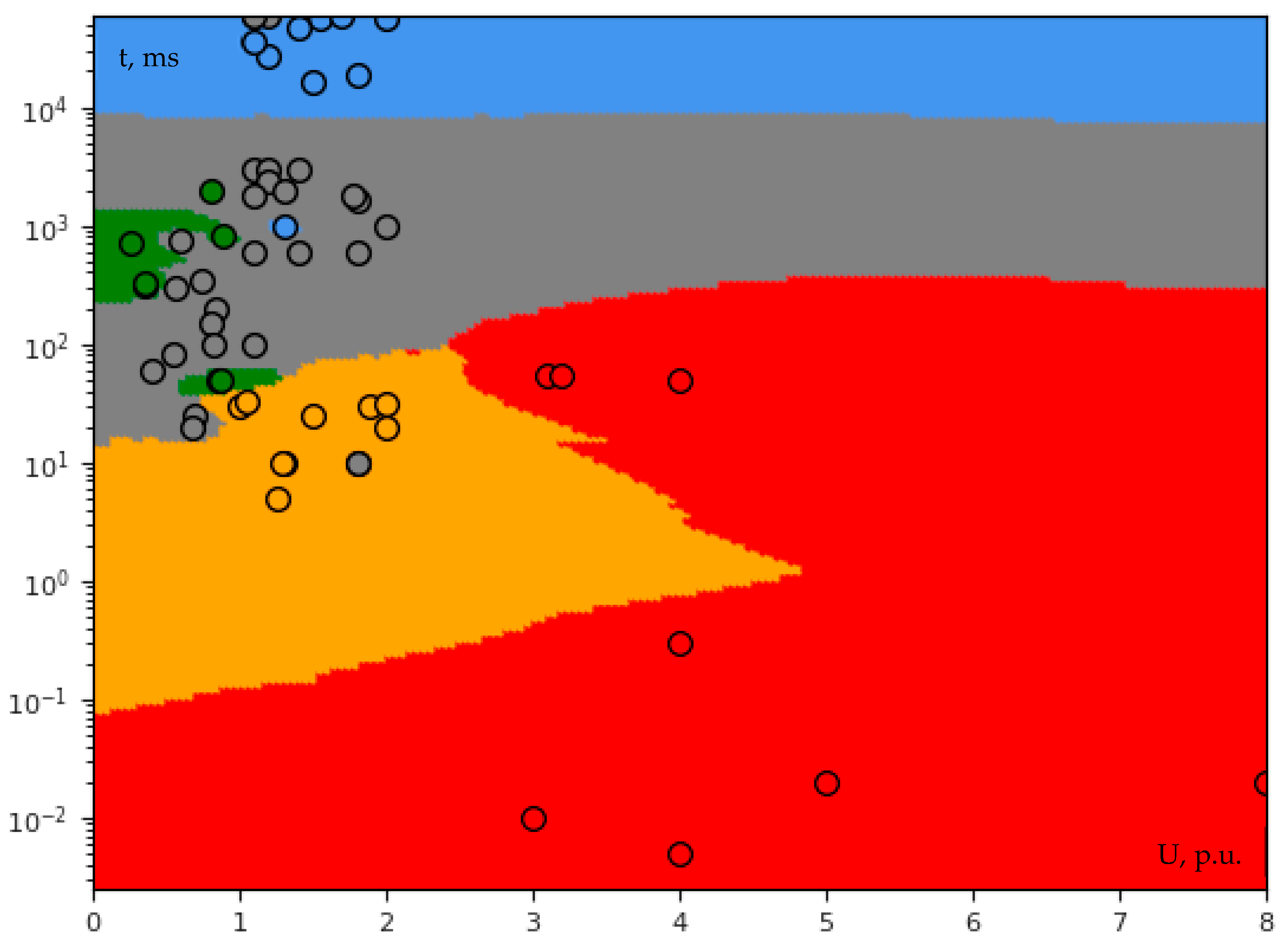
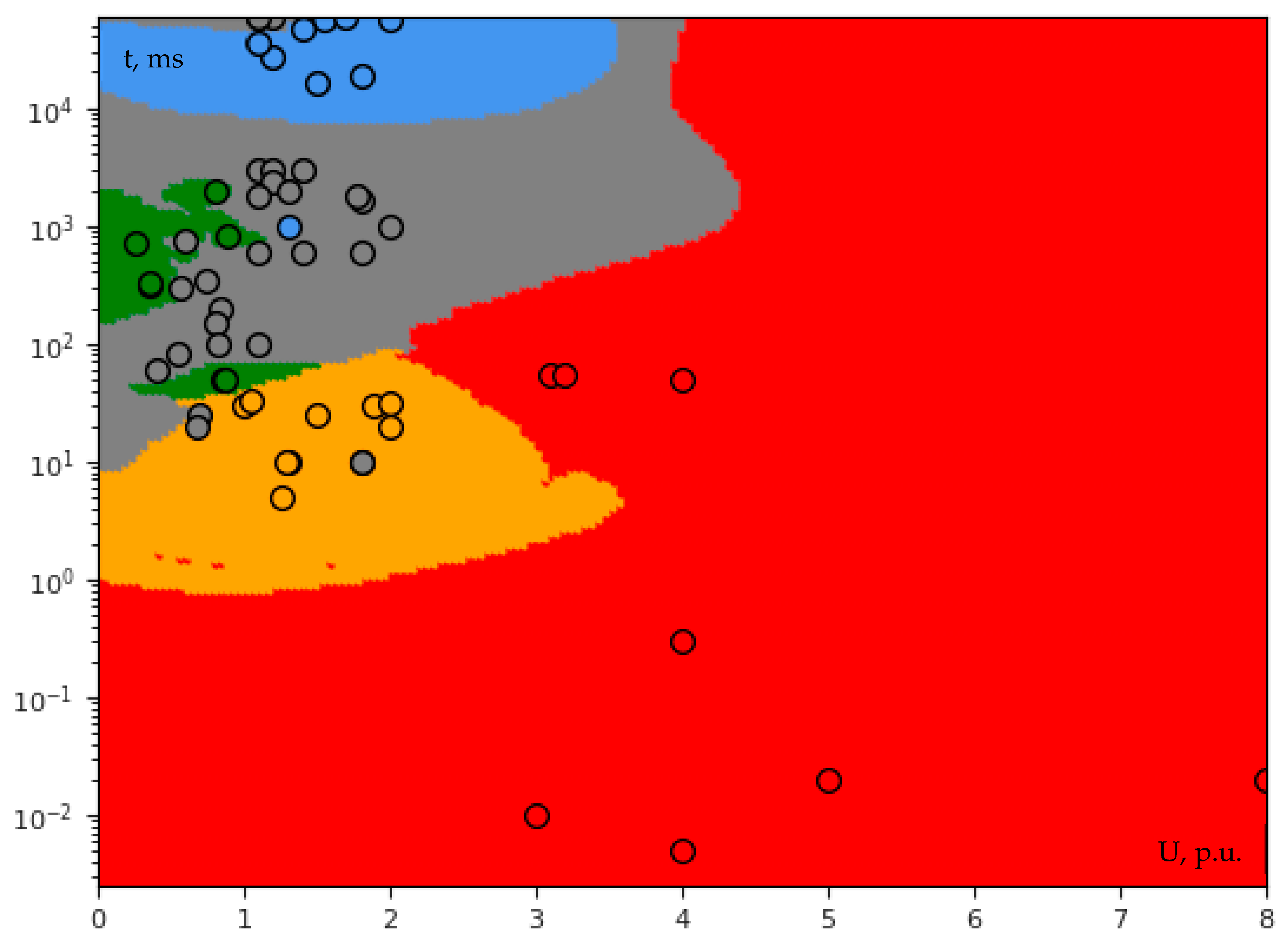
In Section 3.2.2, the idea to transform three-dimensional space into two-dimensional is raised. For this task, we will attempt to apply the alpha–beta (αβγ) transformation, also known as Clarke transformation, which transforms the time domain components of a three-phase system to two components in an orthogonal stationary frame [57]. For a three-phase voltage signal, the mathematical expression of power invariant Clarke transformation takes the following form:

$$\left[\begin{array}{c}{u}_{\alpha }\left(t\right)\\ u_{\beta }\left(t\right)\\ u_{\gamma }\left(t\right)\end{array}\right]=\sqrt{\frac{2}{3}} \left[\begin{array}{ccc}1& -\frac{1}{2}& -\frac{1}{2}\\ 0& \frac{\sqrt{3}}{2}& -\frac{\sqrt{3}}{2}\\ \frac{1}{\sqrt{2}}& \frac{1}{\sqrt{2}}& \frac{1}{\sqrt{2}}\end{array}\right]\left[\begin{array}{c}{u}_a\left(t\right)\\ u_b\left(t\right)\\ u_c\left(t\right)\end{array}\right],$$

(40)

where ${\left[\begin{array}{ccc}{u}_a\left(t\right)& u_b\left(t\right)& u_c\left(t\right)\end{array}\right]}^{\mathrm{T}}$—three-phase voltage $u_{abc}\left(t\right)$; ${\left[\begin{array}{ccc}{u}_{\alpha }\left(t\right)& u_{\beta }\left(t\right)& u_{\gamma }\left(t\right)\end{array}\right]}^{\mathrm{T}}$—corresponding voltage in the αβγ reference plane after the transformation. If the input is symmetrical:

$$\left[\begin{array}{c}{u}_a\left(t\right)\\ u_b\left(t\right)\\ u_c\left(t\right)\end{array}\right]=\left[\begin{array}{c}\sqrt{2}U\cos \theta \left(t\right)\\ \sqrt{2}U\cos \left(\theta \left(t\right)-\frac{2}{3}\pi \right)\\ \sqrt{2}U\cos \left(\theta \left(t\right)+\frac{2}{3}\pi \right)\end{array}\right],$$

(41)

then the output of the transformation is as follows:

$$\left[\begin{array}{c}{u}_{\alpha }\left(t\right)\\ u_{\beta }\left(t\right)\\ u_{\gamma }\left(t\right)\end{array}\right]=\left[\begin{array}{c}\sqrt{3}U\cos \theta \left(t\right)\\ \sqrt{3}U\sin \theta \left(t\right)\\ 0\end{array}\right],$$

(42)

where $U$—rms voltage; and $\theta \left(t\right)$—generic time-varying angle (can also be set to $\omega t$). Therefore, in the case of a balanced signal, the third component is equal to zero. This is the main reason of our choice, which makes it potentially promising. However, in the case of asymmetry, the third component is not equal to zero (see Section 3.2.2 and Appendix A for more information about results interpretation and decisions made).

We also noticed that the result of the power invariant Clarke transformation (Equation (40)) is similar to a power invariant direct-quadrature-zero (DQZ) transformation when the α-axis is aligned to the d-axis and the angle $\theta$ is equal to zero:

$$\left[\begin{array}{c}{u}_d\left(t\right)\\ u_q\left(t\right)\\ 0\end{array}\right]=\sqrt{\frac{2}{3}} \left[\begin{array}{ccc}\cos \theta & \cos \left(\theta -\frac{2\pi }{3}\right)& \cos \left(\theta +\frac{2\pi }{3}\right)\\ -\sin \theta & -\sin \left(\theta -\frac{2\pi }{3}\right)& -\sin \left(\theta +\frac{2\pi }{3}\right)\\ \frac{1}{\sqrt{2}}& \frac{1}{\sqrt{2}}& \frac{1}{\sqrt{2}}\end{array}\right]\left[\begin{array}{c}{u}_a\left(t\right)\\ u_b\left(t\right)\\ u_c\left(t\right)\end{array}\right],$$

(43)

where $\theta$—angle between the α-axis and d-axis (equal to zero); ${\left[\begin{array}{ccc}{u}_a\left(t\right)& u_b\left(t\right)& u_c\left(t\right)\end{array}\right]}^{\mathrm{T}}$—three-phase voltage $u_{abc}\left(t\right)$; ${\left[\begin{array}{ccc}{u}_d\left(t\right)& u_q\left(t\right)& 0\end{array}\right]}^{\mathrm{T}}$—corresponding voltage in DQZ reference plane after the transformation. This transformation is the product of Clarke transformation and Park transformation. The latter converts the components of the orthogonal stationary αβγ frame to an orthogonal rotating DQZ reference frame [57,58]. The rotation angular velocity of both the d-axis and q-axis is equal to $\omega$, and the angle $\theta$ is equal to $\omega t$: in this particular case, when $\theta$ is equal to zero, then $\omega$ is also zero.

3. Results

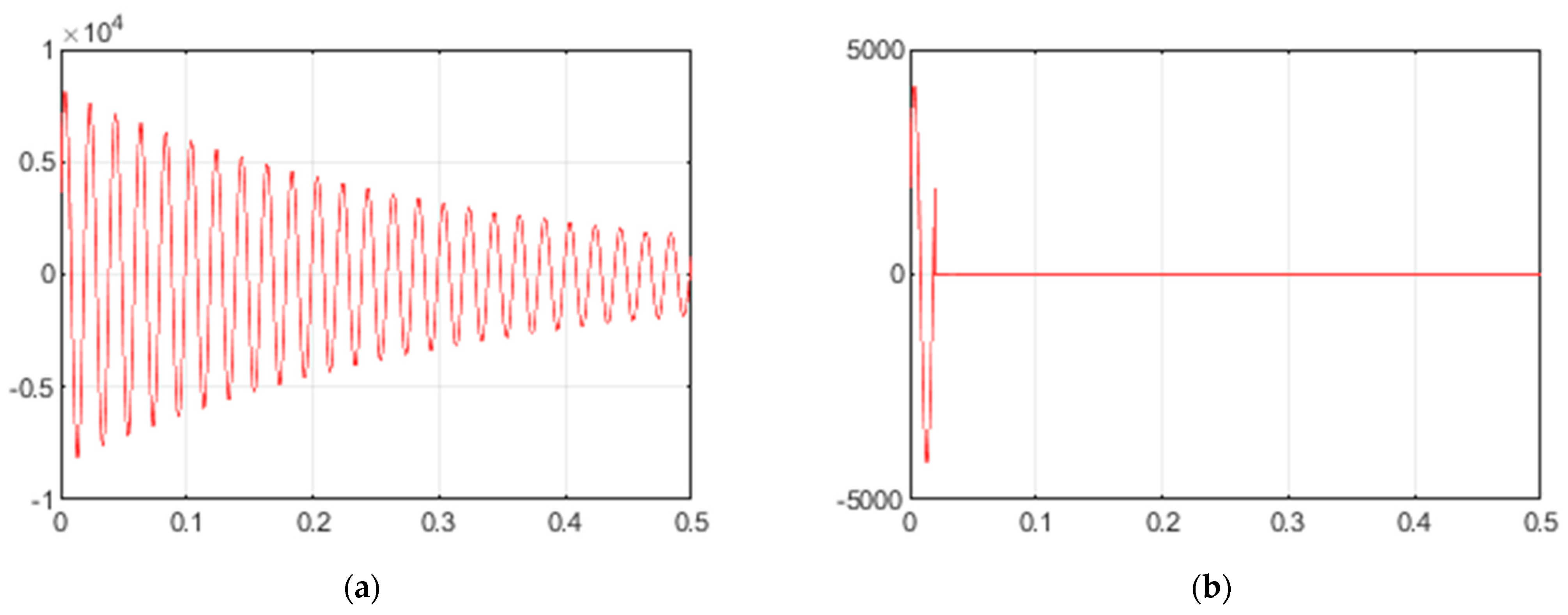
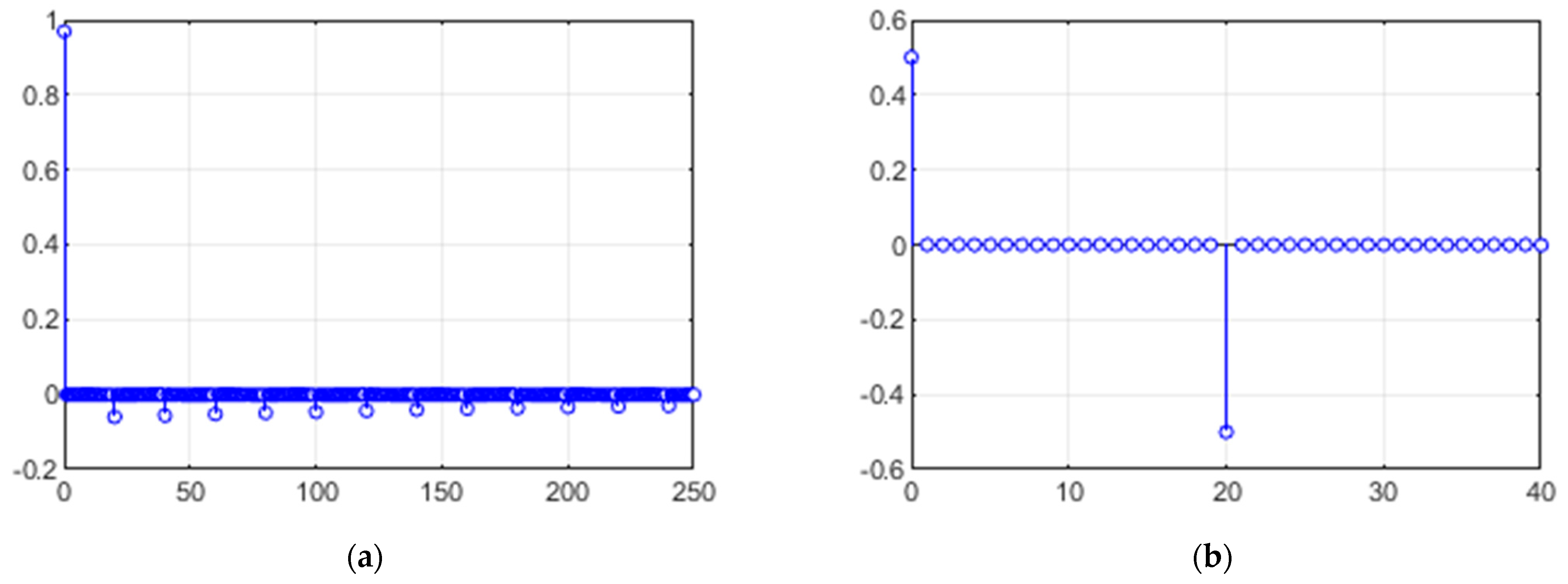
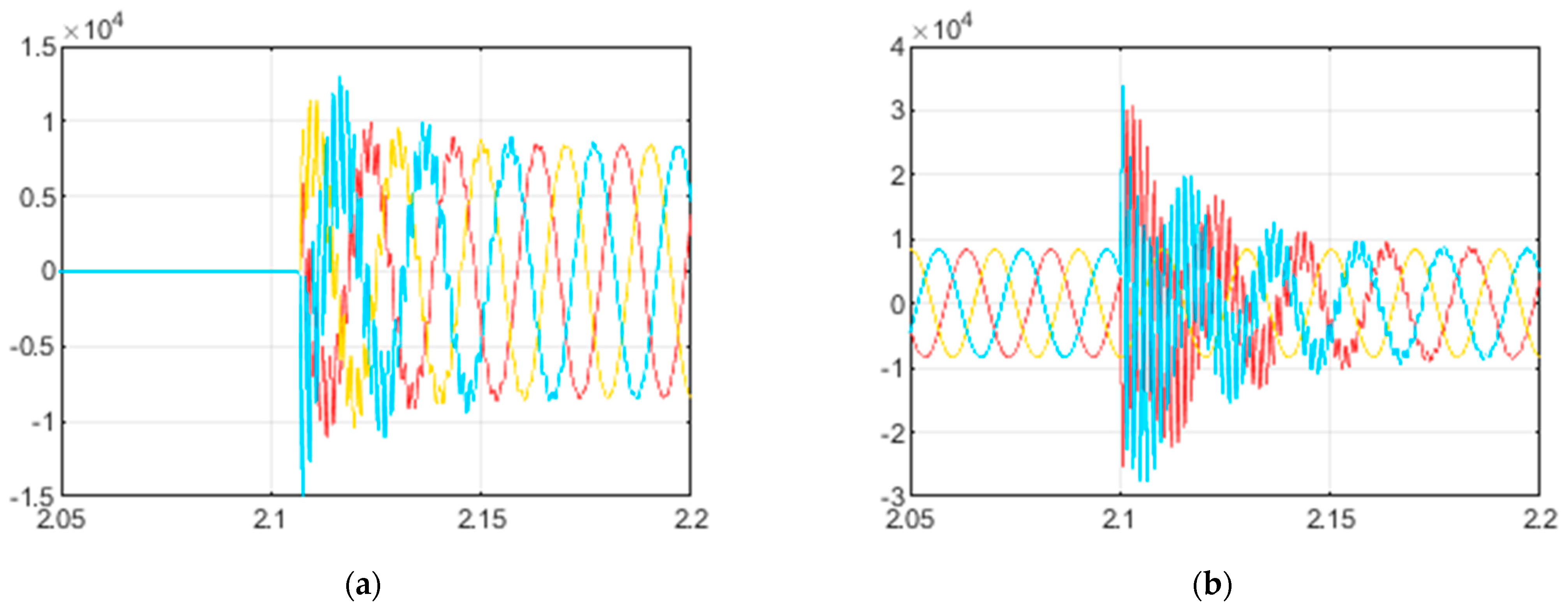
3.1. Shelving Filter

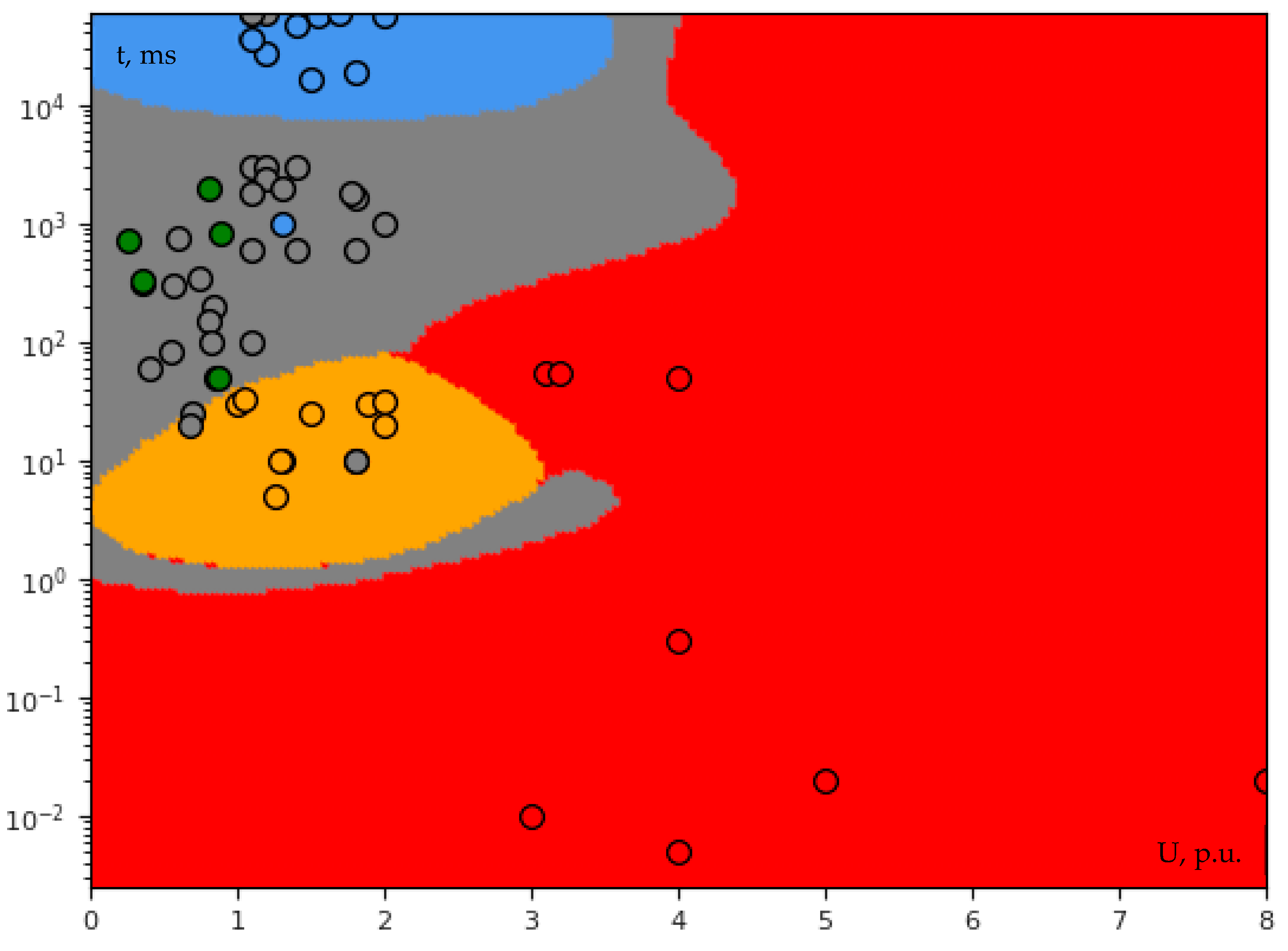
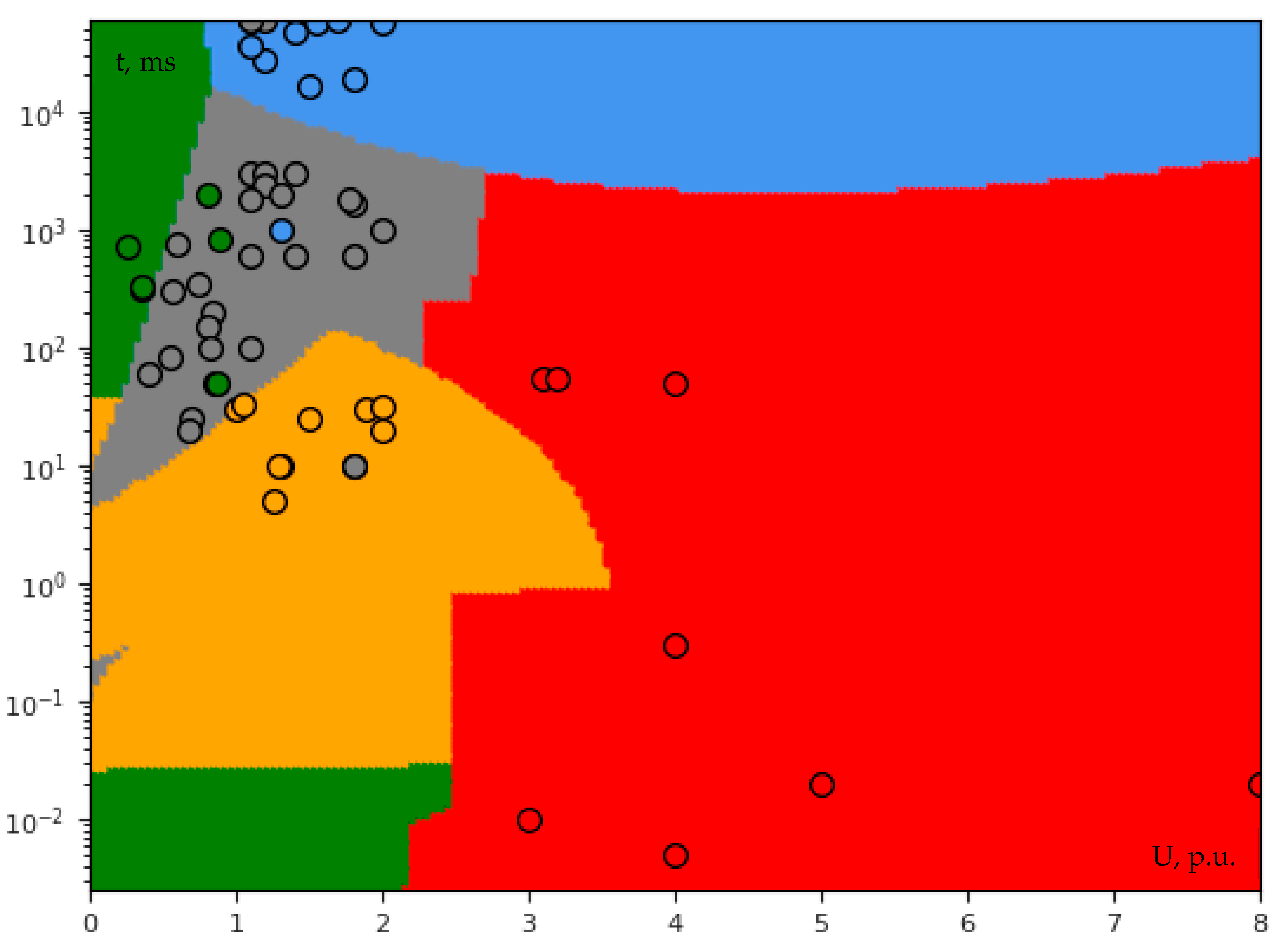
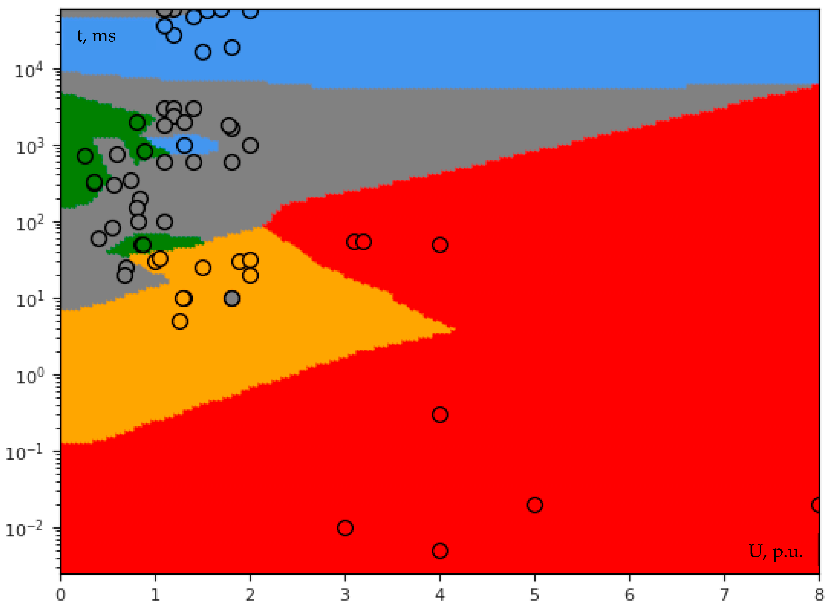
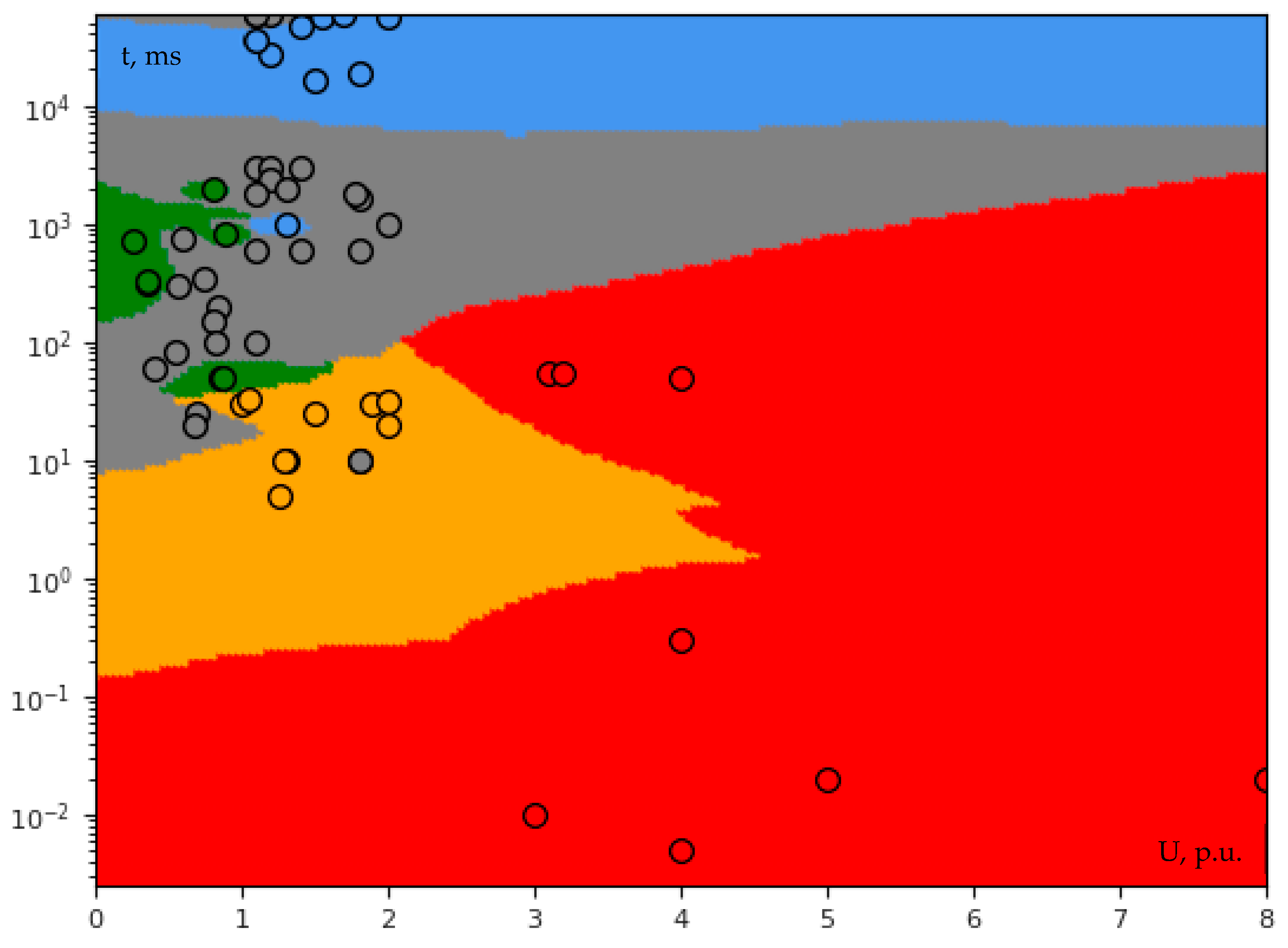
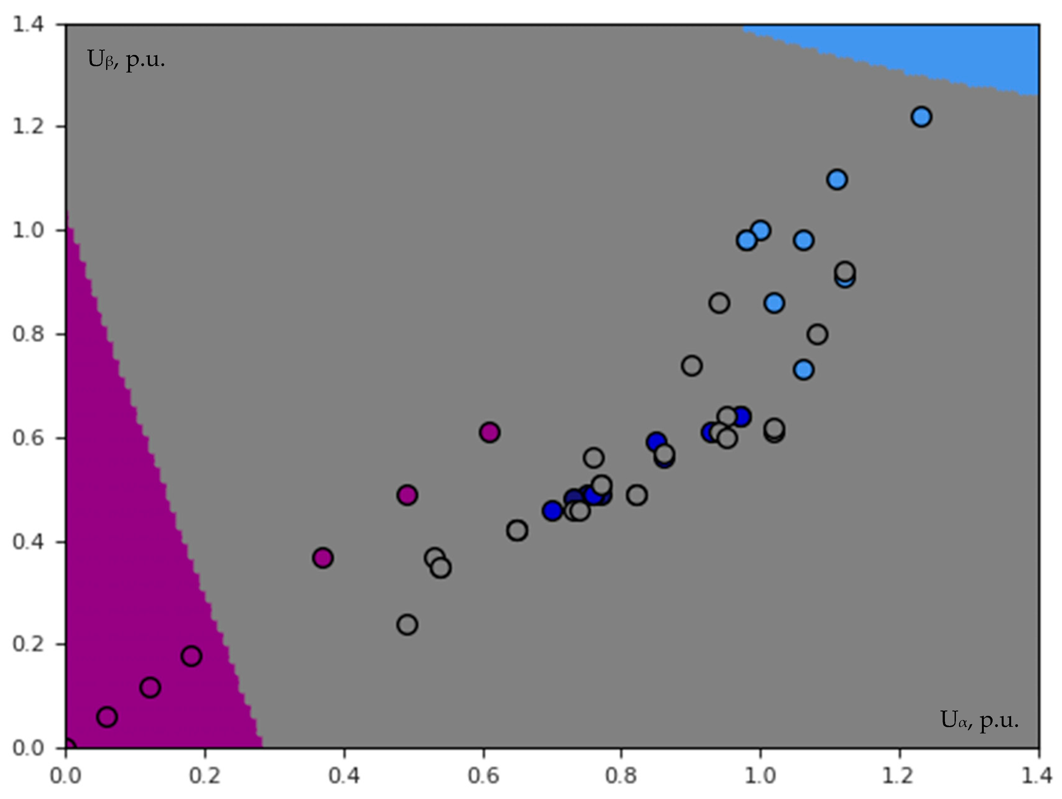
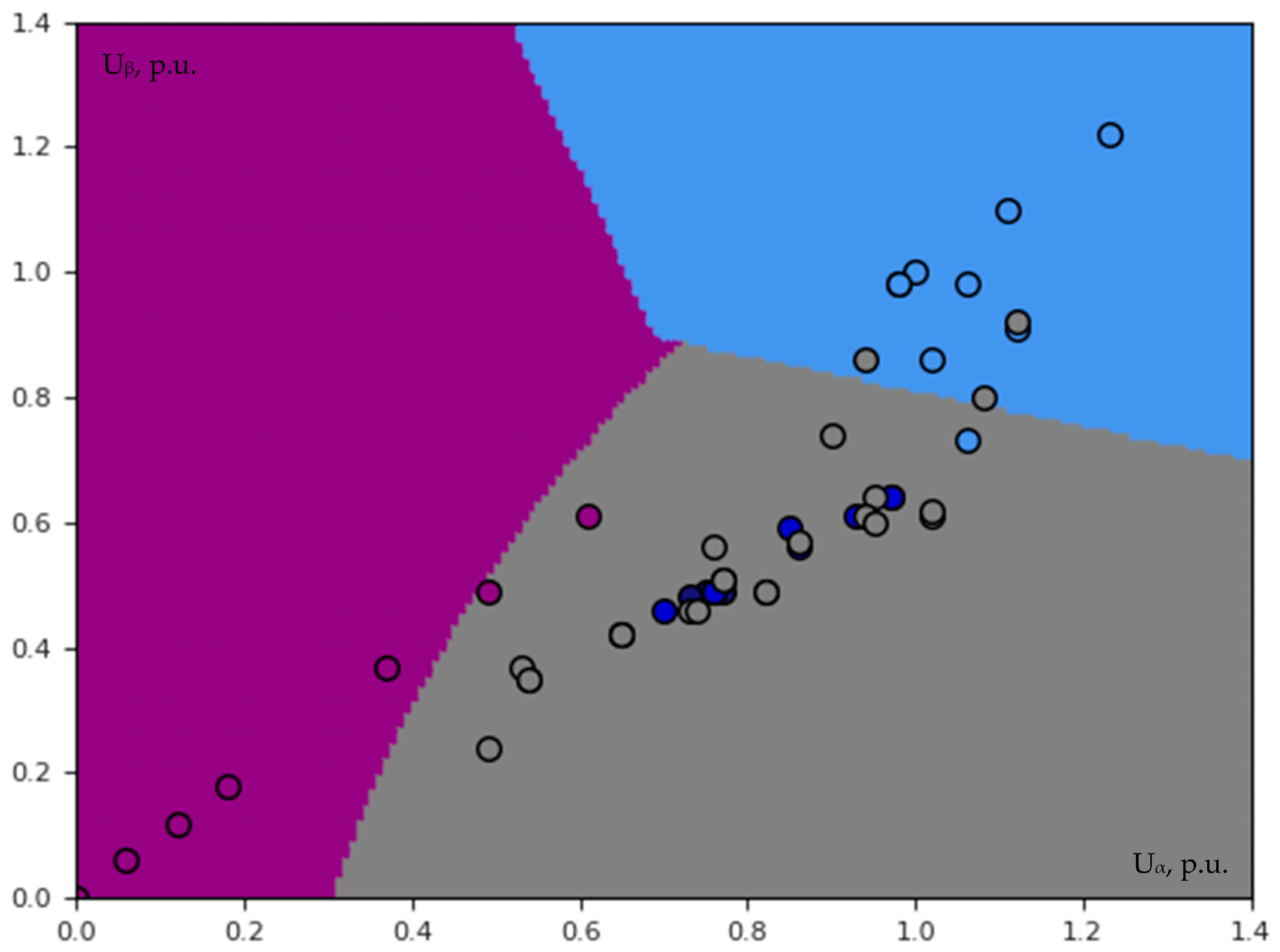
Let us begin with the examination of a filter transient response to a 50 Hz signal of 10 kV phase-to-ground voltage. When the stopband width $\Delta f$ is set to 1 Hz, the filter’s transient process lasts a relatively long time—longer than 0.5 s (Figure 8a), which may result in a high risk to conceal an overall majority of PQ events. Therefore, in an iterative way, it has been figured out that the shortest process is observed when $\Delta f$ is equal to 25 Hz (Figure 8b). An analogous tendency is also observed in the filter impulse response (Figure 9).

In the pole–zero plot (Figure 10), a stopband width $\Delta f$ corresponds with the distance between the pole and zero across the respective radius of the unit circle. The system remains stable in the both cases (i.e., impulse response approaches zero), because all poles are inside the unit circle. Since all zeros are on the boundary of the unit circle, maximal attenuation is achieved.

In Figure 11, both types of voltage transients, described in Section 2.1.1 and Section 2.1.2, and their filtering results are given. The first is a commutation transient caused by a 10 kV line switching on (Figure 11a), which is described by Equations (1)–(5). The second is an atmospheric transient which propagated from a 110 kV grid to a 10 kV grid (Figure 11b). This oscillation is the result of the grid response to the lightning impulse, modeled by Equation (8), when the current peak value $I_m$ is 205 kA, rise time $t_1$ is 21 μs, and fall time $t_2$ is 300 μs. The occurrence frequency of such an impulse is lower than 0.01. Its electric charge is 87 C, which is lower than (but close to) the 100 C used in IEC 62305-1:2010 for the highest lightning protection level from the first positive impulse. The filtering results of the transients in phase A (red curve) are given in Figure 11c–f. When $\Delta f$ is 1 Hz, in the case of the commutation transient, it is clearly seen (examining both magnitude and time) that the true signal is hidden beyond the heavy transient response (Figure 11c), but in the case of the atmospheric transient—the difference between true and output signals is not visually clear (Figure 11d). On the other hand, when $\Delta f$ is 25 Hz and the transient response is the lightest (shortest), the signal distortions are clearly seen in Figure 11e,f, which cannot be recognized as a desirable result.

A signal’s distortion can be evaluated from the magnitude and phase frequency response of the digital filter (Figure 12): the magnitude and phase of signal frequency components are less distorted when $\Delta f$ is equal to 1 Hz (especially phase); however, as it has been shown in Figure 8, its transient response is heavier than in the case when $\Delta f$ is equal to 25 Hz.

In the case of RMS variations, the filter is not useful because the frequency of voltage sag/swell is 50 Hz. The example of a single-phase fault is given in Figure 13. Considering the above, it is decided to continue the research with the fundamental component included.

3.2. Classification

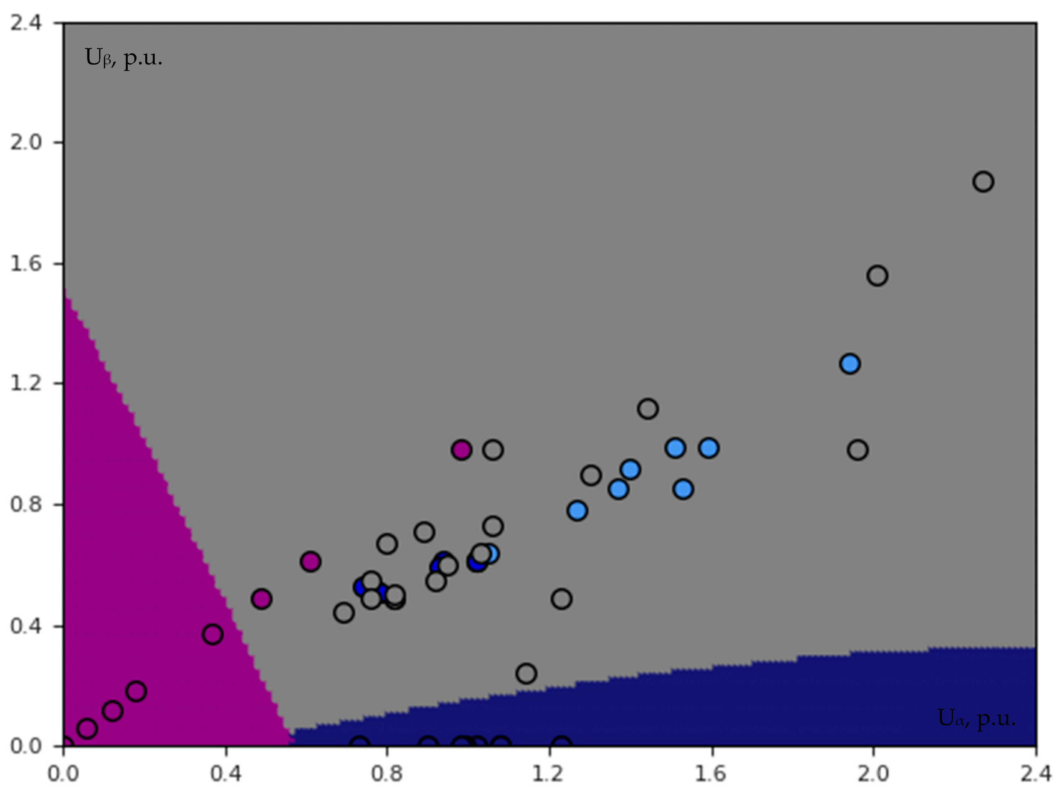
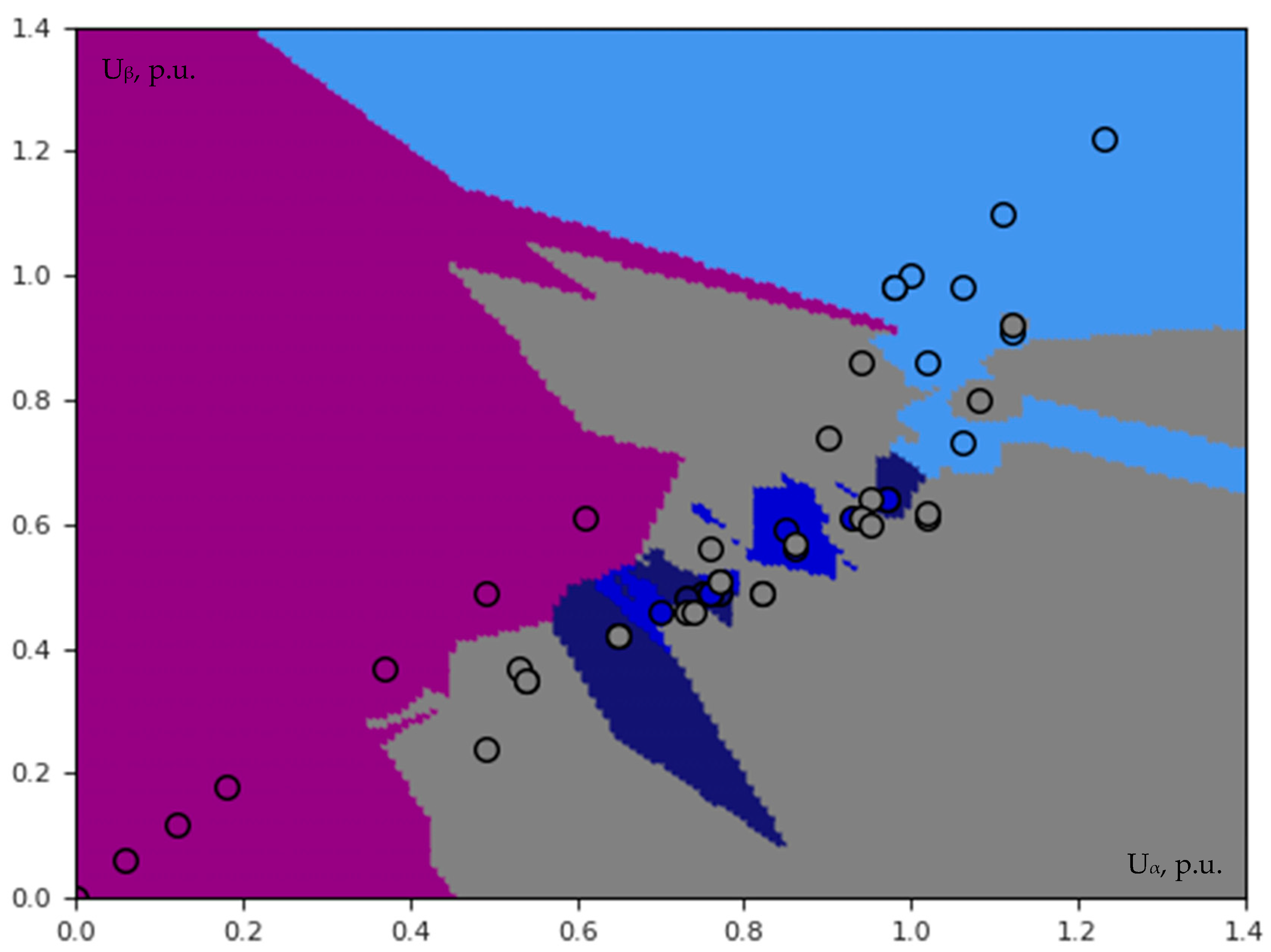
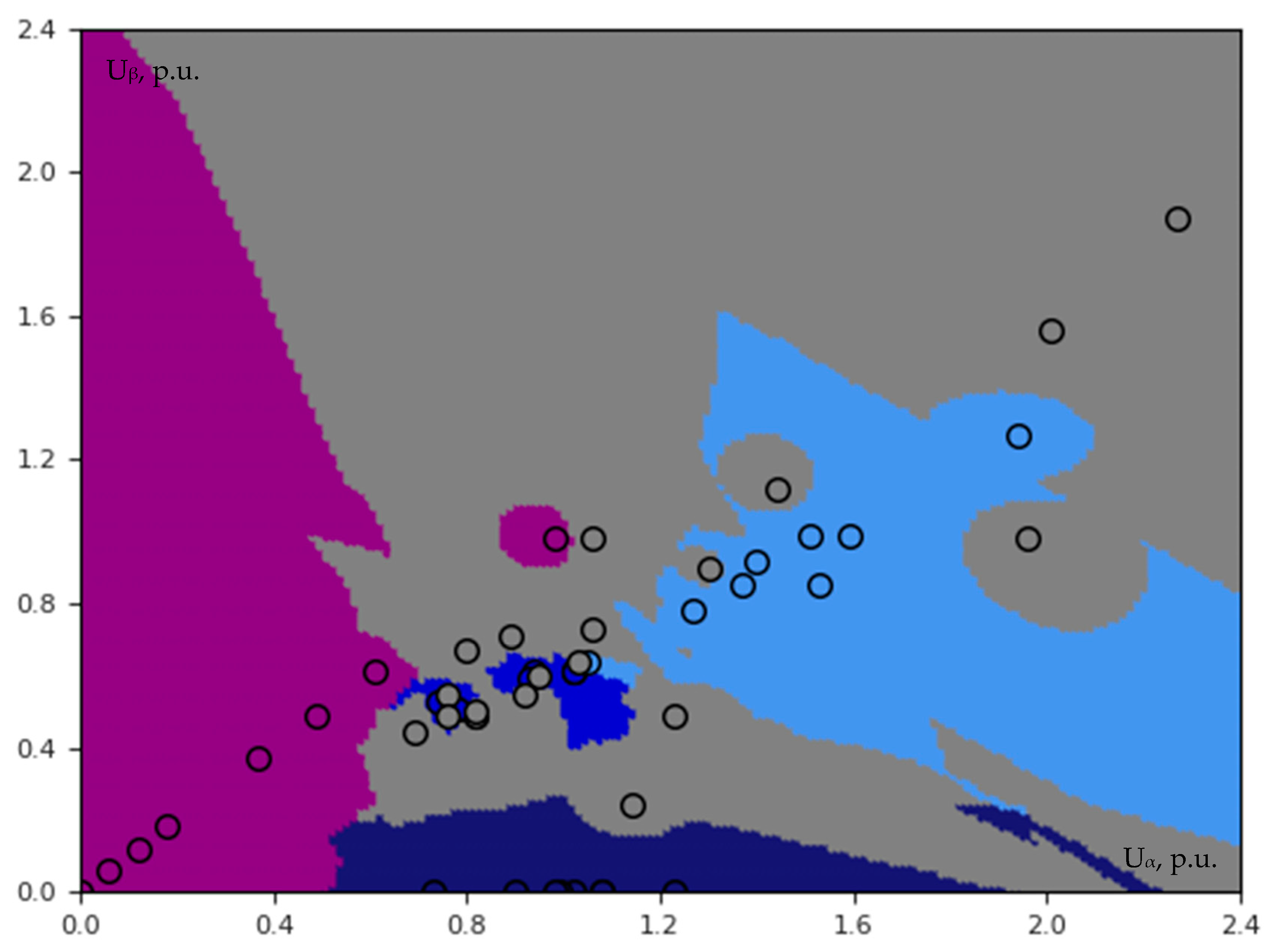
3.2.1. Single-Voltage Classification

The investigation is started with single-voltage array analysis, which is part of a three-phase system. In this case, the feature vector has the following form:

$$x_i={\left[\begin{array}{cc}{U}_i& t_i\end{array}\right]}^{\mathrm{T}},$$

(44)

where $U$—voltage (either phase-to-phase or phase-to-ground), p.u.; $t$—duration, ms. In

Table 2. Characteristic data points of the training set.

Group	Data
Atmospheric transient	8 p.u.	5 p.u.			4 p.u.				4 p.u.			4 p.u.			3.2 p.u.				3.1 p.u.				3 p.u.
	0.02 ms	0.02 ms			50 ms				0.3 ms			0.005 ms			55 ms				55 ms				0.01 ms
Commutation transient	2 p.u.	2 p.u.		1.88 p.u.			1.8 p.u.			1.5 p.u.		1.3 p.u.		1.29 p.u.			1.25 p.u.			1.05 p.u.				1 p.u.
	31 ms	20 ms		30 ms			10 ms			25 ms		10 ms		10 ms			5 ms			33 ms				30 ms
Single-phase short circuit	2 p.u.	1.8 p.u.		1.7 p.u.			1.55 p.u.			1.5 p.u.		1.4 p.u.		1.3 p.u.			1.2 p.u.			1.1 p.u.				1.1 p.u.
	55 s	19 s		60 s			56 s			16 s		46 s		1000 ms			27 s			60 s				35 s
Electric motor starting	0.88 p.u.	0.87 p.u.				0.85 p.u.					0.8 p.u.		0.35 p.u.					0.35 p.u.				0.25 p.u.
	800 ms	50 ms				50 ms					2000 ms		327 ms					307 ms				710 ms
Not categorized	2 p.u.	1.8 p.u.		1.8 p.u.			1.8 p.u.			1.78 p.u.		1.4 p.u.		1.4 p.u.			1.3 p.u.			1.2 p.u.				1.2 p.u.
	1000 ms	1600 ms		600 ms			10 ms			1780 ms		3000 ms		600 ms			60 s			3000 ms				2300 ms
	1.2 p.u.	1.1 p.u.		1.1 p.u.			1.1 p.u.			1.1 p.u.		1.1 p.u.		0.84 p.u.			0.82 p.u.			0.8 p.u.				0.74 p.u.
	2000 ms	60 s		3000 ms			1800 ms			600 ms		10 ms		200 ms			100 ms			150 ms				340 ms
	0.7 p.u.		0.68 p.u.					0.6 p.u.				0.57 p.u.				0.55 p.u.					0.4 p.u.
	25 ms		20 ms					750 ms				290 ms				80 ms					60 ms

, the features are given exactly in this form. Four PQ event groups are labeled (atmospheric transient, commutation transient, single-phase short circuit, and electric motor starting), and the fifth group is for uncategorized events without any label assigned (gray zone). The results of both SVM and KNN, obtained in Python, are given in Figure 14, Figure 15, Figure 16, Figure 17, Figure 18, Figure 19 and Figure 20. The characteristic points are marked with the outline.

Despite the background in Section 2.1, an additional explanation should be given about single-phase short circuits. The Lithuanian MV grid operates in either isolated or compensated neutral mode; thus, two phase-to-ground voltage swells along with one interruption are inherent to the single-phase fault. It can last several hours, because even under these circumstances, the grid is still able to ensure power supply to end-users (see [2,9] for more information). Since the size of our time window is limited to 1 min (according to the definition of short-duration RMS variation given by IEEE Std 1159-2019), during a single-phase fault, each point will be at 1 min, and after that, it will be once at a random time (which depends on the moment of the disconnection). Thus, the magnitude of voltage swell is given according to the simulation results obtained in [9], but its duration is determined with a random number generator. It should be noted that such circumstances tighten the dynamic range requirements.

Typically, machine learning requires a large database; however, it is not essential to this task because the PQ database can be enlarged with a random number generator (see Section 4.3 for more details). Since one of the goals is to avoid both abnormal range and extreme values during data generation (see Section 4.2 for more information about data quality), competency and experience remain much more important, and these skills can be acquired mostly during only PQ monitoring campaigns. It is noteworthy that the information about the typical range of the characteristics of PQ events can be found only in few sources, and one of them is IEEE Std 1159-2019.

Firstly, it seems that KNN performs better than SVM with a soft margin (in all SVM cases, the regularization parameter $C$ is equal to 1). For example, in Figure 14 (it shows SVM results with linear kernel), both all green and all yellow points are outside their zones, which does not mean that these zones are inappropriate but indicates insufficient coverage (span). On the contrary, this problem is not encountered in the case of KNN, but that does not necessarily mean that the best possible solution was found. Secondly, it is clear that a single either SVM or KNN cannot deal with the overlapping in the voltage–duration plane, for example: (1) an atmospheric transient (especially damped) can have the same characteristics as a commutation transient (but not vice versa); however, the grid operator must be able to identify such a discrepancy by itself; (2) no events are expected (possible) in the upper right corner of Figure 14, Figure 15, Figure 16, Figure 17, Figure 18, Figure 19 and Figure 20; (3) despite the fact that a voltage swell is inherent not only to a single-phase fault but also to a two-phase-to-ground fault, the overlapping zone is not large because two-phase-to-ground faults are usually disconnected as soon as possible (say up to 2–3 s but typically within a few tens of milliseconds). Also, it is obvious that the approach can be expanded by adding more groups, but at present, this is hardly implemented due to insufficient knowledge and experience in the field. Thirdly, a few words must be written about classification accuracy. As mentioned in Section 1, most authors affirm that their classification accuracy is close to perfect. However, in the field of PQ, it actually depends on either the validation or test set: since each zone (category) covers at least some part of the correct (expected) range, it is not problematic to either adjust or select a test set similar to the training set with maintained realism and solid argumentation and thereby achieve desired (high) accuracy. Fourthly, in spite of the fact that each zone covers its correct range, it also can fall in the regions where it is unexpected; however, this issue does not necessarily have a significant effect on the performance (accuracy): for example, currently, it is not possible to confirm nor deny that the amplitude of any commutation transient can be higher than 4 p.u. (contrary to Figure 17, Figure 18 and Figure 19), and it can be confirmed that the amplitude of any voltage swell during a single-phase fault is not expected to be higher than 3 p.u. and lower than 1 p.u. (contrary to Figure 14, Figure 15, Figure 16, Figure 17, Figure 18, Figure 19 and Figure 20). Lastly, in order to implement the task, the EN 50160:2010 requirement for the multiphase aggregation had to be rejected (see Section 4.1 for more details). Also, currently, the data of the entire power system (consisting of HV, MV and LV grids) is plotted on one plane: on the one hand, such an approach does not have serious drawbacks and, on the other hand, the data segregation by, for example, either voltage lever or neutral mode could (slightly) improve the performance.

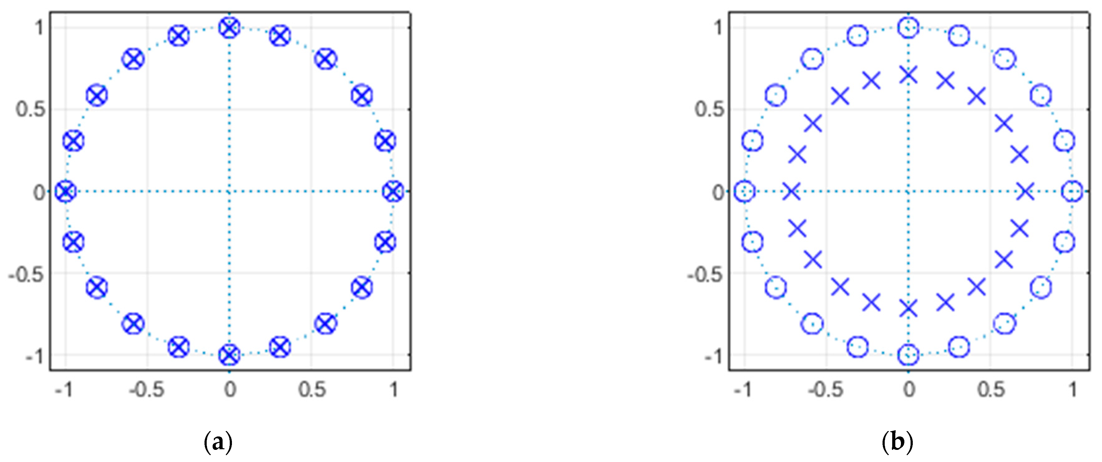
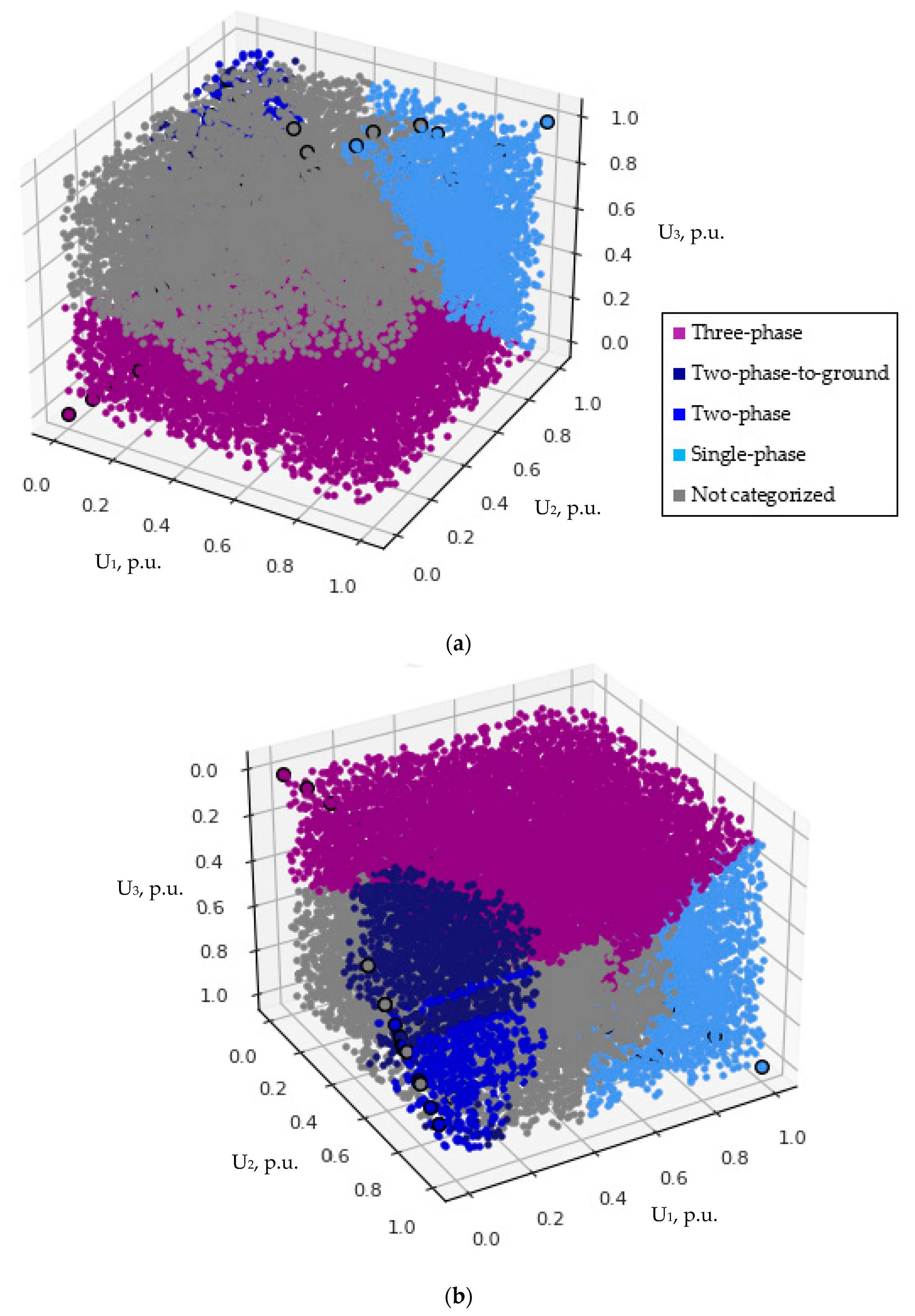
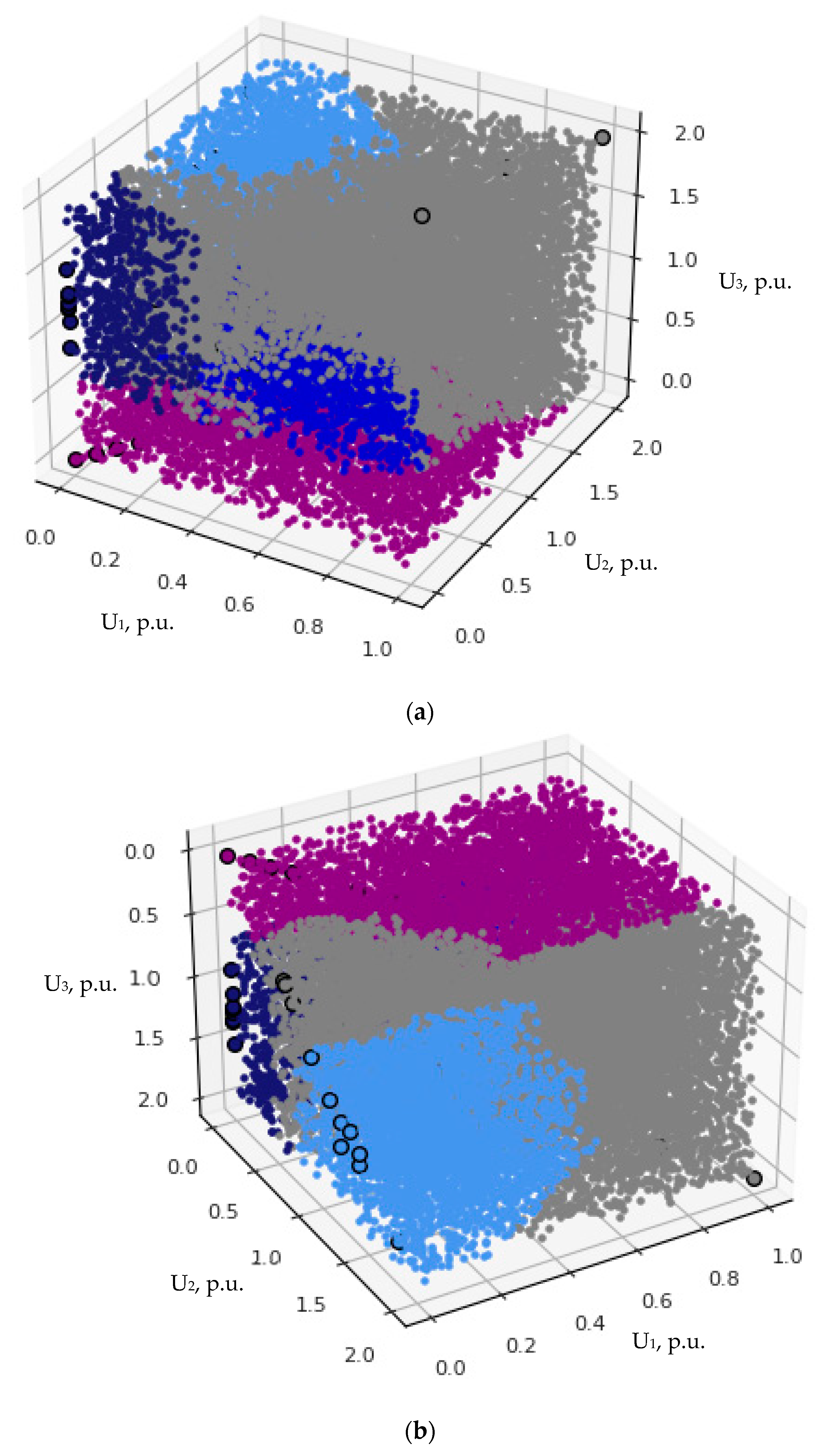
3.2.2. Three-Dimensional Voltage Classification

An asymmetrical short circuit cannot be described with any single voltage value; therefore, the approach must be based on three-dimensional voltage classification. In this case, the feature vector has the following form:

$$x_i={\left[\begin{array}{ccc}{U}_1{}_i& U_2{}_i& U_3{}_i\end{array}\right]}^{\mathrm{T}},$$

(45)

where $U_1$, $U_2$ and $U_3$ are either phase-to-phase or phase-to-ground voltages at a fault node arranged in ascending order, p.u. On the one hand, the order of numbers in the feature array is not important; on the other hand, in this paper, the arrangement in ascending order is preferred for research purposes. Analogously to Section 3.2.1, for this case, data quality is more important than quantity.

It is noteworthy that no three-dimensional voltage classification was found in the existing PQ literature, and most likely the reason for this is the absence of comprehensive investigations of asymmetrical faults (and, respectively, database), as has been argued by [9]. Both training sets (

Table 3. Phase-to-phase voltage characteristic data points of the training set.

Group	Data
Three-phase short circuit	0.8 (0.98)		0.5 (0.61)		0.4 (0.49)		0.3 (0.37)		0.15 (0.18)		0.1 (0.12)		0.05 (0.06)		0.0 (0.00)
	0.8 (0.98)		0.5 (0.61)		0.4 (0.49)		0.3 (0.37)		0.15 (0.18)		0.1 (0.12)		0.05 (0.06)		0.0 (0.00)
	0.8 (0.00)		0.5 (0.00)		0.4 (0.00)		0.3 (0.00)		0.15 (0.00)		0.1 (0.00)		0.05 (0.00)		0.0 (0.00)
Two-phase-to-ground short circuit	0.0 (0.97)		0.0 (0.77)		0.0 (0.76)		0.0 (0.76)		0.0 (0.75)		0.0 (0.73)		0.0 (0.65)		0.0 (0.54)
	0.9 (0.64)		0.7 (0.49)		0.7 (0.49)		0.7 (0.49)		0.69 (0.49)		0.68 (0.48)		0.6 (0.42)		0.5 (0.35)
	0.9 (0.52)		0.72 (0.41)		0.71 (0.41)		0.7 (0.40)		0.7 (0.40)		0.68 (0.39)		0.6 (0.35)		0.5 (0.29)
Two-phase short circuit	0.0 (0.97)		0.0 (0.93)		0.0 (0.86)		0.0 (0.85)		0.0 (0.77)		0.0 (0.76)		0.0 (0.70)		0.0 (0.65)
	0.9 (0.64)		0.86 (0.61)		0.8 (0.56)		0.79 (0.59)		0.72 (0.51)		0.7 (0.49)		0.65 (0.46)		0.6 (0.42)
	0.9 (0.52)		0.86 (0.49)		0.8 (0.46)		0.79 (0.46)		0.72 (0.42)		0.7 (0.40)		0.65 (0.38)		0.6 (0.35)
Single-phase short circuit	1.0 (1.23)		0.9 (1.11)		0.82 (1.00)		0.8 (0.98)		0.7 (1.06)		0.7 (1.12)		0.7 (1.02)		0.6 (1.06)
	1.0 (1.22)		0.9 (1.10)		0.82 (1.00)		0.8 (0.98)		0.9 (0.98)		0.8 (0.91)		0.7 (0.86)		0.6 (0.73)
	1.0 (0.00)		0.9 (0.00)		0.82 (0.00)		0.8 (0.00)		0.9 (0.12)		1.0 (0.15)		0.9 (0.12)		1.0 (0.23)
Not categorized	0.7 (1.12)	0.6 (0.94)		0.6 (1.08)		0.6 (0.90)		0.52 (0.95)	0.5 (1.02)	0.5 (0.94)		0.4 (1.02)		0.4 (0.82)		0.4 (0.73)
	0.8 (0.92)	0.8 (0.86)		0.7 (0.80)		0.6 (0.74)		0.52 (0.64)	0.5 (0.61)	0.5 (0.61)		0.6 (0.62)		0.4 (0.49)		0.4 (0.49)
	1.0 (0.15)	0.8 (0.12)		1.0 (0.21)		0.8 (0.12)		0.9 (0.22)	1.0 (0.29)	0.9 (0.23)		1.0 (0.31)		0.8 (0.23)		0.7 (0.17)
	0.3 (0.76)	0.3 (0.82)		0.3 (0.53)		0.2 (0.49)		0.1 (0.95)	0.1 (0.74)	0.0 (0.86)		0.0 (0.77)		0.0 (0.65)		0.0 (0.54)
	0.6 (0.56)	0.5 (0.49)		0.3 (0.37)		0.2 (0.24)		0.8 (0.60)	0.6 (0.46)	0.8 (0.57)		0.72 (0.51)		0.6 (0.42)		0.5 (0.35)
	0.7 (0.21)	0.8 (0.25)		0.5 (0.12)		0.5 (0.17)		0.9 (0.44)	0.7 (0.32)	0.8 (0.46)		0.72 (0.42)		0.6 (0.35)		0.5 (0.29)

and

Table 4. Phase-to-ground voltage characteristic data points of the training set.

Group	Data
Three-phase short circuit	0.8 (0.98)		0.5 (0.61)		0.4 (0.49)		0.3 (0.37)		0.15 (0.18)		0.1 (0.12)		0.05 (0.06)		0.0 (0.00)
	0.8 (0.98)		0.5 (0.61)		0.4 (0.49)		0.3 (0.37)		0.15 (0.18)		0.1 (0.12)		0.05 (0.06)		0.0 (0.00)
	0.8 (0.00)		0.5 (0.00)		0.4 (0.00)		0.3 (0.00)		0.15 (0.00)		0.1 (0.00)		0.05 (0.06)		0.0 (0.00)
Two-phase-to-ground short circuit	0.0 (1.23)		0.0 (1.08)		0.0 (1.08)		0.0 (1.02)		0.0 (0.99)		0.0 (0.98)		0.0 (0.90)		0.0 (0.73)
	0.0 (0.00)		0.0 (0.00)		0.0 (0.00)		0.0 (0.00)		0.0 (0.00)		0.0 (0.00)		0.0 (0.00)		0.0 (0.00)
	1.5 (0.87)		1.32 (0.76)		1.3 (0.76)		1.25 (0.72)		1.22 (0.70)		1.2 (0.69)		1.1 (0.64)		0.9 (0.52)
Two-phase short circuit	0.5 (1.02)		0.5 (1.02)		0.5 (1.02)		0.5 (0.94)		0.48 (0.93)		0.43 (0.74)		0.42 (0.78)		0.4 (0.78)
	0.5 (0.61)		0.5 (0.61)		0.5 (0.61)		0.5 (0.61)		0.48 (0.59)		0.43 (0.53)		0.42 (0.51)		0.4 (0.51)
	1.0 (0.29)		1.0 (0.29)		1.0 (0.29)		0.9 (0.23)		0.9 (0.24)		0.69 (0.15)		0.75 (0.19)		0.8 (0.19)
Single-phase short circuit	0.0 (1.94)		0.0 (1.59)		0.0 (1.51)		0.0 (1.40)		0.0 (1.53)		0.0 (1.37)		0.0 (1.27)		0.0 (1.05)
	1.8 (1.27)		1.4 (0.99)		1.4 (0.99)		1.3 (0.92)		1.2 (0.85)		1.2 (0.85)		1.1 (0.78)		0.9 (0.64)
	1.8 (1.04)		1.5 (0.84)		1.4 (0.81)		1.3 (0.75)		1.5 (0.79)		1.3 (0.72)		1.2 (0.69)		1.0 (0.55)
Not categorized	1.0 (2.27)	0.8 (2.01)		0.8 (1.96)		0.8 (1.06)		0.6 (1.44)	0.6 (1.06)	0.58 (0.89)		0.52 (1.03)		0.5 (0.80)		0.4 (0.92)
	2.0 (1.87)	1.7 (1.56)		0.8 (0.98)		0.8 (0.98)		1.2 (1.12)	0.6 (0.73)	0.58 (0.71)		0.52 (0.64)		0.6 (0.67)		0.5 (0.55)
	2.0 (0.58)	1.8 (0.55)		2.0 (0.69)		0.9 (0.06)		1.3 (0.38)	1.0 (0.23)	0.8 (0.13)		1.0 (0.28)		0.7 (0.10)		0.9 (0.26)
	0.4 (0.76)	0.4 (1.23)		0.4 (0.82)		0.4 (0.82)		0.3 (1.30)	0.3 (0.82)	0.2 (1.14)		0.1 (0.95)		0.0 (0.76)		0.0 (0.69)
	0.5 (0.55)	0.4 (0.49)		0.4 (0.49)		0.4 (0.49)		1.1 (0.90)	0.5 (0.50)	0.2 (0.24)		0.8 (0.60)		0.7 (0.49)		0.62 (0.44)
	0.7 (0.15)	1.3 (0.52)		0.8 (0.23)		0.7 (0.23)		1.2 (0.49)	0.8 (0.25)	1.3 (0.64)		0.9 (0.44)		0.7 (0.40)		0.62 (0.36)

) are based on the results of this paper with all its limitations that are inherent to the inductive reasoning method, including the fact that the results were obtained in the BRELL-based test scheme (different network properties in other countries may have different impacts on the patterns of PQ events). Also, it is clear that phase-to-phase and phase-to-ground cases must be investigated separately except for the case of a symmetrical fault due to the following axiom established by [9]:

Axiom 1. 

In the case of a three-phase fault, both phase-to-phase and phase-to-ground voltage sag depths are equal and independent of neutral mode.

The training set in the form of Equation (45) is given in Table 3 and Table 4. All four types of short circuits are included. Please note that the group label is assigned only to the voltage of the fault node (regardless of the scenario), while the voltages of the rest nodes fall in the gray zone. In Table 4, the same phase-to-ground voltage swells of a single-phase short circuit can be noticed as in Table 2. In addition, each feature vector after Clarke transformation is given in parentheses. Please note that the transformation output depends on the order of elements in the input vector, and this is important for this research because the third element of the output is discarded.

The results in three-dimensional space are given in Figure 21 and Figure 22. As in the previous case, the characteristic points from Table 3 and Table 4 have the outlines.

Calculations in three-dimensional space were carried out only with KNN because it turned out to be more suitable in Section 3.2.1. This also will be realized later (in this section) after transforming it to two-dimensional space. The range of phase-to-phase voltage is up to 1 p.u., while the range of phase-to-ground voltage is up to 2 p.u. In Python, each calculation took up to 5 min in three-dimensional space (including both training and display steps) and up to 1 min in two-dimensional space (the base frequency of the 4-core processor is 3.50 GHz, RAM—16 GB).

It is difficult to analyze and interpret Figure 21 and Figure 22; thus, let us examine the zones of the characteristic points separately. The results of both phase-to-phase and phase-to-ground cases, obtained in MATLAB, are shown in Figure 23. The theoretical background of the used equations along with their parameters is given in Section 2.5.1: planes that do not coincide with a coordinate hyperplane are colored; a counterclockwise rotation is represented by a positive rotation angle, while a clockwise rotation is represented by a negative rotation angle. The findings convince that the idea of using the ascending order was superb, enabling the observation of many interesting tendencies:

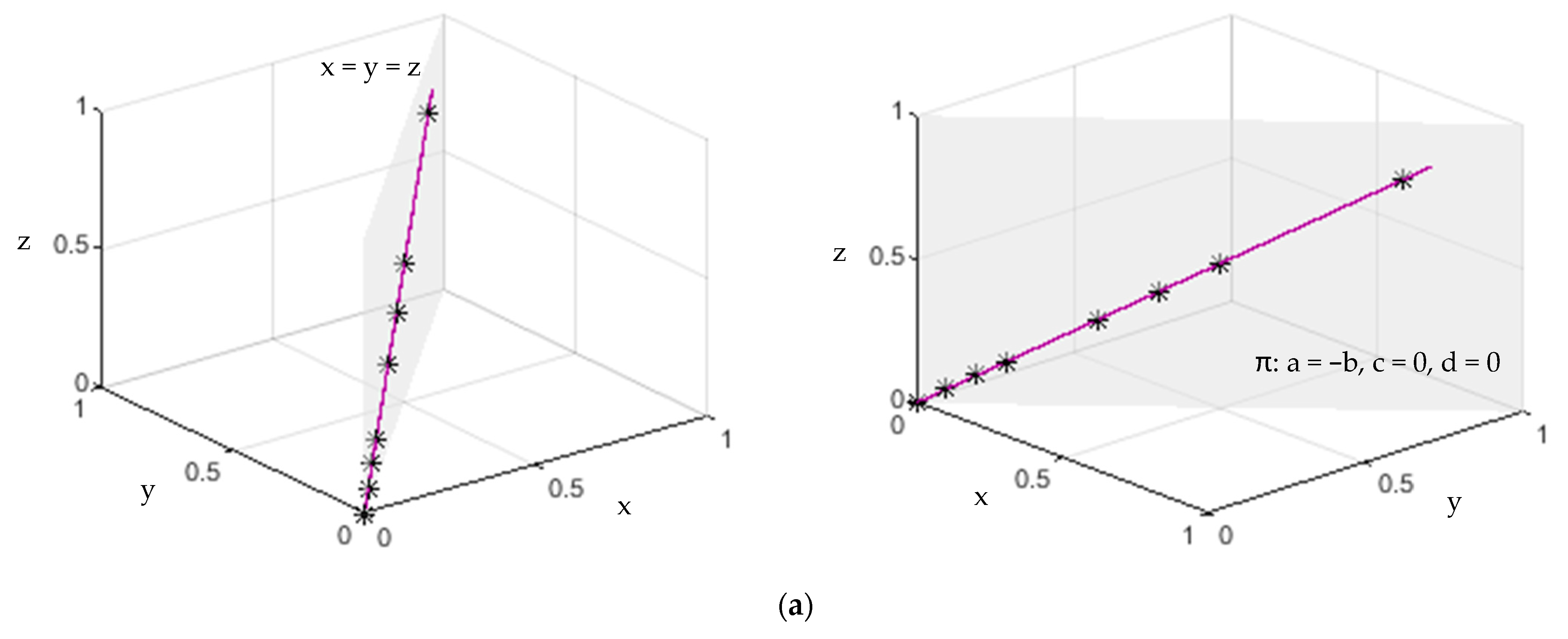
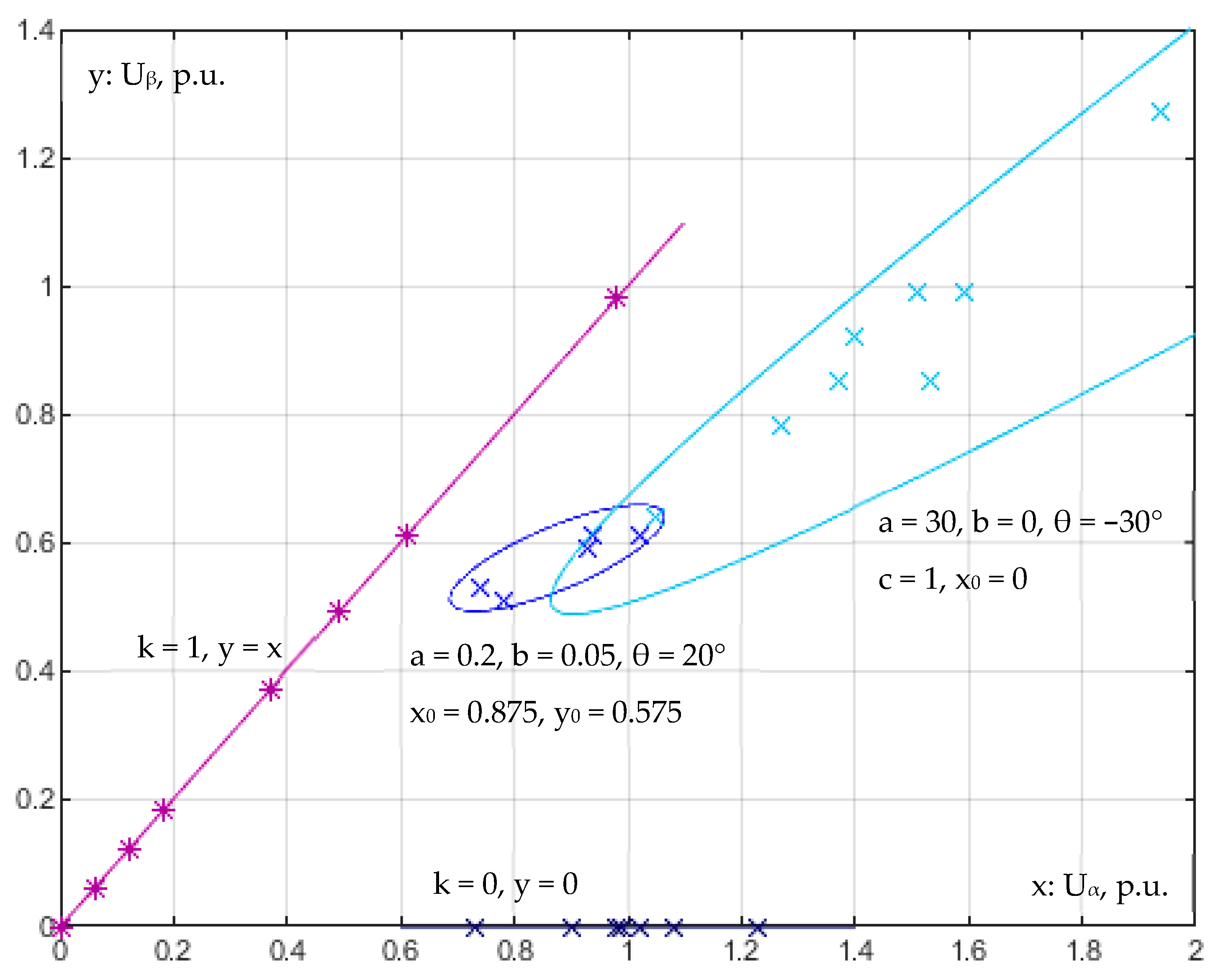
• In the case of a three-phase fault (Figure 23a), all points lie on the line belonging to the plane which forms the angles of 45° with both abscissa and ordinate.
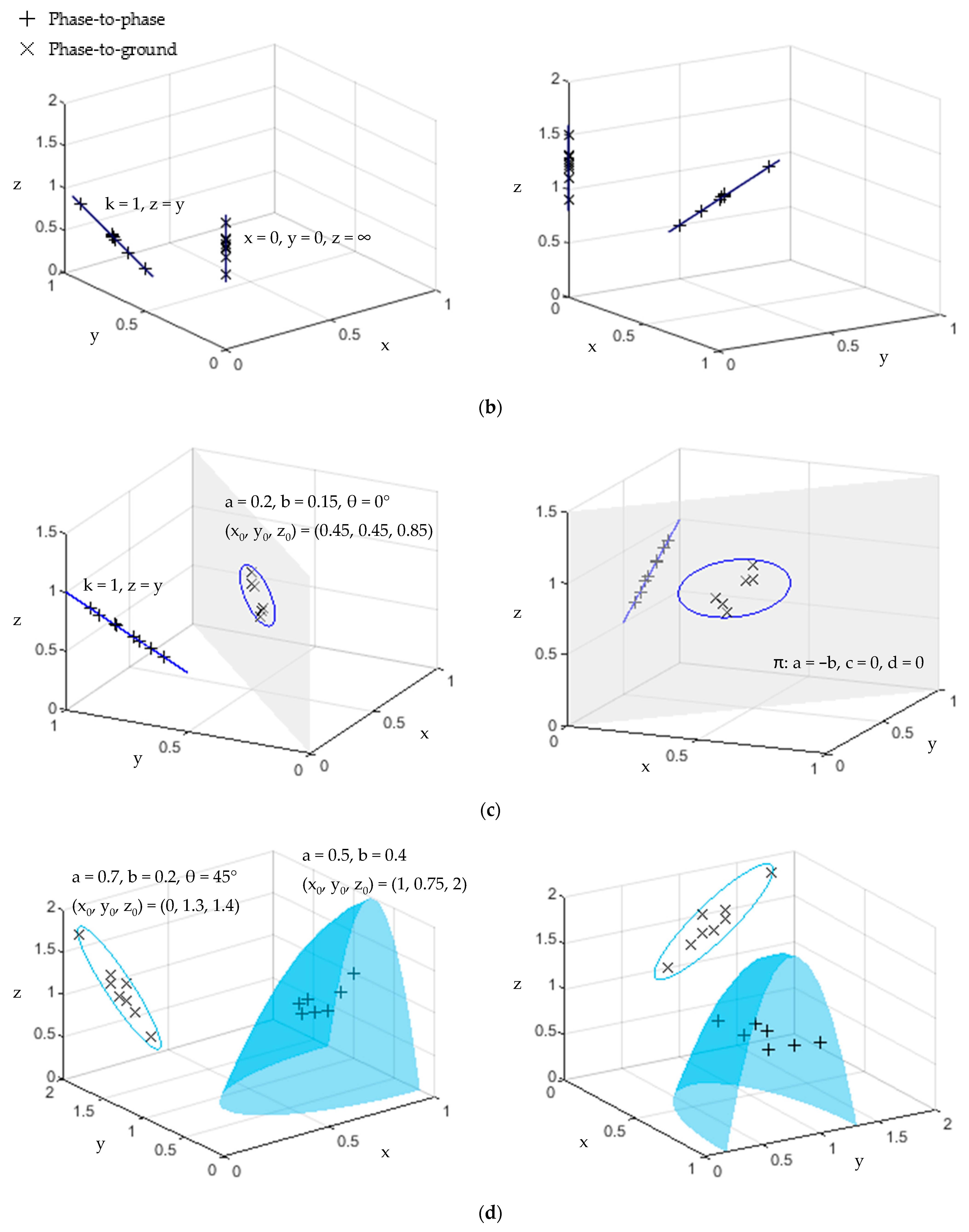
• In the case of a two-phase-to-ground fault (Figure 23b), all points (of both phase-to-phase and phase-to-ground voltages) belong to the same coordinate hyperplane, i.e., are coplanar (see Equation (34)), which is defined by the pair of ordinate and applicate.
• In the case of a two-phase fault (Figure 23c), the phase-to-phase pattern is identical to the case of a two-phase-to-ground fault, while phase-to-ground points are encircled with the ellipse lying in the plane which forms the angles of 45° with both the abscissa and ordinate (analogously to the case of a three-phase fault).
• In the case of a single-phase fault (Figure 23d), phase-to-phase points are covered with one half of the paraboloid, while phase-to-ground points are encircled with the ellipse lying in the coordinate hyperplane defined by the pair of ordinate and applicate.

As in the previous case, please note that the data are not segregated by grid voltage or neutral mode, and despite this, the trends still appeared. Such analysis and findings would be not be possible with the multiphase aggregation required by EN 50160:2010. The next stage is the elimination of inductive reasoning limitations, which should be performed by foreign authors. Then, two outcomes are possible: (1) if it turns out that the findings of this paper are universal, it would mean a great leap forward toward the successful completion of the classification task; (2) if the results are different, the geometry of clusters’ boundaries should be modified accordingly as long as it will be required for the universalization. Please note that there is an option to alter the currently set parameters of the used ellipses and paraboloid, and the applied approach is not the only way to define a feature cluster’s border (see Section 4.3.1).

As has been mentioned above, it is obvious that the three-dimensional feature space of Figure 21 and Figure 22 is difficult to analyze (especially visually). Respectively, the analysis of larger n-dimensional spaces will possibly be even more complicated. For this purpose, we create a new method to transform a three-dimensional feature space into a two-dimensional. The method is based on Clarke transformation (see Section 2.5.2) and implemented in MATLAB/Simulink. Transformation output is given in the brackets of Table 3 and Table 4, whereas the results in the αβ plane, which is obtained by discarding component γ, are given in Figure 24, Figure 25, Figure 26, Figure 27 and Figure 28 (where the colors are kept the same as in the legend of Figure 21). More information about the transformation procedure can be found in Appendix A. It is noteworthy that the proposed method is completely appropriate for the analysis of short circuits; however, this does not indicate the suitability for universal application to various tasks (but it may be). In Figure 24, Figure 25 and Figure 26, similarly as in Section 3.2.1, it is clearly seen that the performance of SVM is not satisfying enough with both regularization parameter $C$ values—1 (which corresponds to a soft margin) and 10 (which corresponds to a hard margin). Luckily, KNN works much better (Figure 27 and Figure 28). In addition, similarly as in Figure 23, the geometric analysis of the clusters in the αβ plane is given in Figure 29 and Figure 30. It can be noticed that phase-to-ground voltage is more informative than the phase-to-phase voltage due to smaller overlapping; nevertheless, in order to enhance the performance, both voltages should be assessed regardless of EN 50160:2010. Moreover, it would be greatly beneficial to identify areas where no data points are expected (e.g., the upper left corner).

4. Discussion

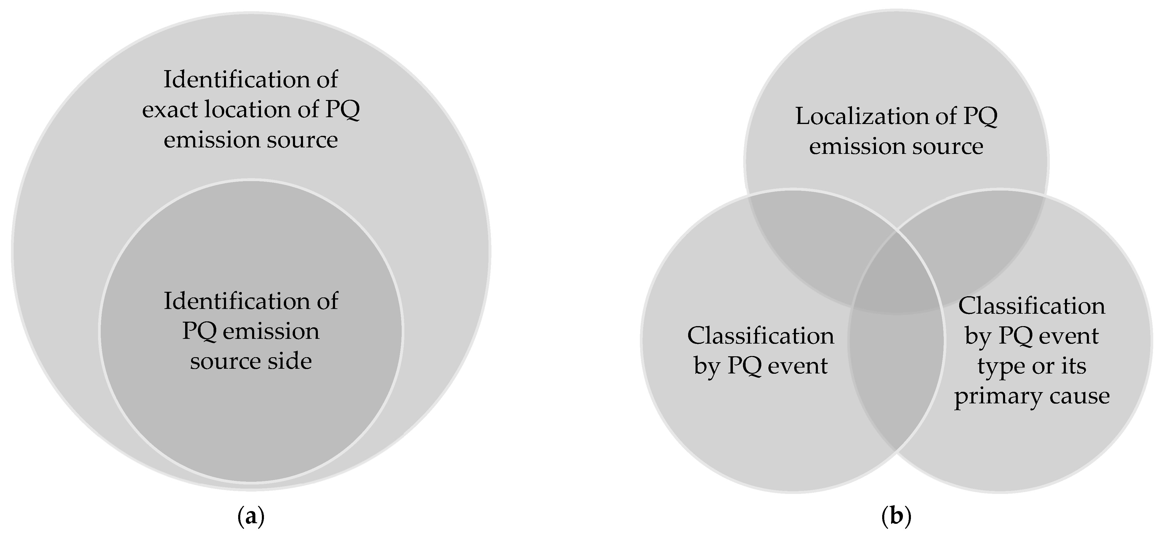
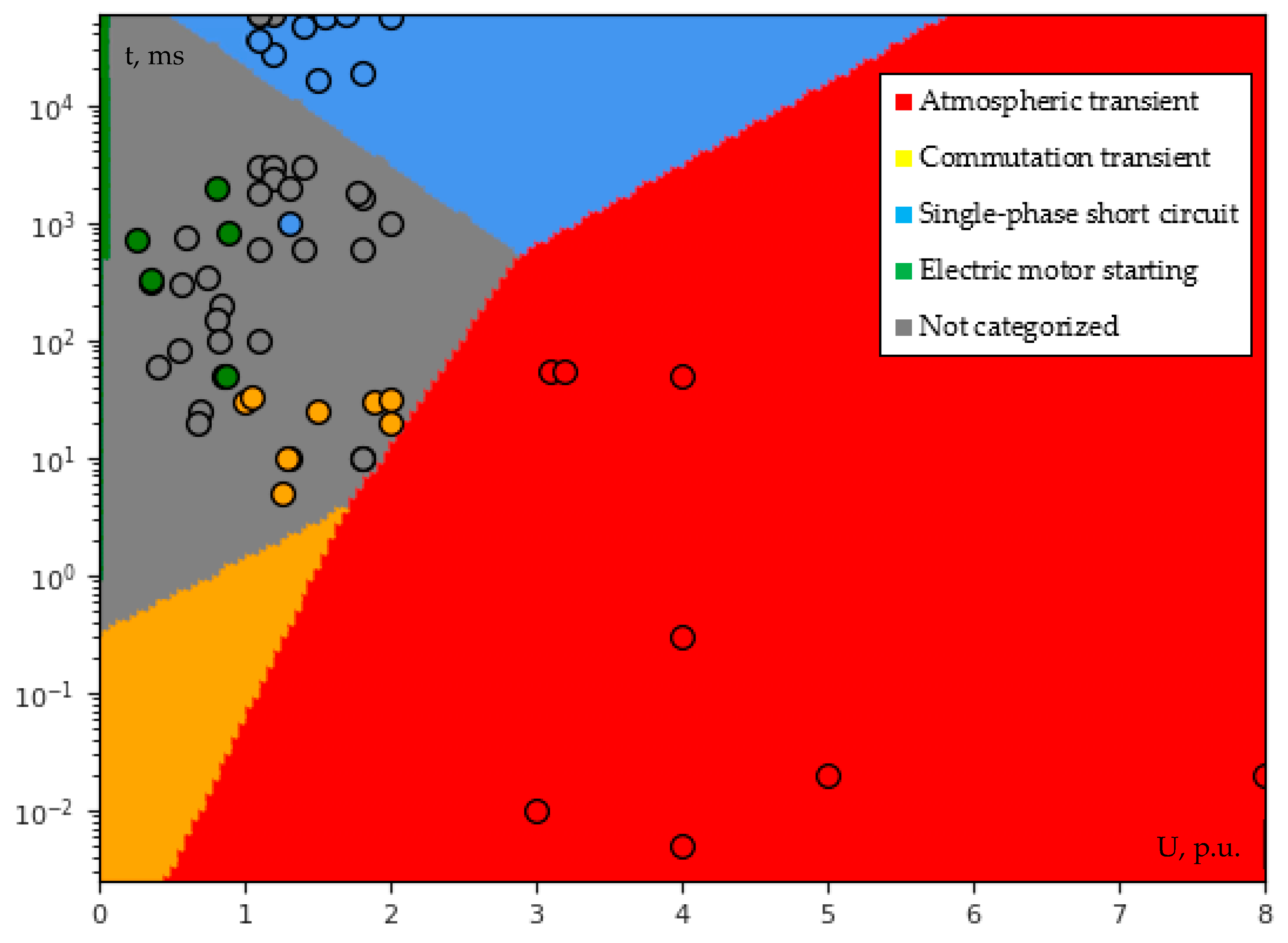
4.1. PQ Events Assessment

A lot of universally unsolved issues in the field of PQ events assessment are considered to be highly limiting factors for the further research and application of AI algorithms [2]. Some of these issues, particularly those regarding voltage sag assessment, which were noticed during the PQ monitoring campaign in the Lithuanian DSO grid (see Section 2.1.3), are discussed in this section. Many of them can be treated as PQ legislation gaps. Appropriate amendments in EN 50160:2010, IEC 61000-4-30:2015, IEEE Std 1159-2019, IEEE Std 1564-2014 and other relevant standards (documents) are essential to accelerate the development and usefulness of PQ monitoring systems. At the moment, there is no similar discussion to this in the existing PQ literature.

Firstly, it has been noticed that the RMS voltage of some voltage sags is time-varying (multistage), i.e., they have a stepped shape. The example is given in Figure 31: a voltage sag event was recorded on 6 March 2019 on the 10 kV side of the 35/10 kV substation (located in Širvintos municipality). Therefore, although the stepped shape can be characterized according to EN 50160:2010, i.e., with a single residual voltage and duration (as in Section 2.1.3), such an approach seems to be inaccurate and inappropriate because it does not reflect any information about the voltage sag profile. IEC 61000-4-30:2015 also briefly mentions this aspect, i.e., that the envelopes of both voltage sag and swell are not necessarily rectangular. This is one of the main drawbacks of currently the most popular method of the voltage–duration plane (e.g., as in Figure 2a). In our opinion, the problem can be solved by using the voltage sag energy characteristic, which is defined in IEEE Std 1564-2014 as follows:

$$E=\underset{0}{\overset{T}{{\displaystyle \int }}}\left(1-\frac{U^2\left(t\right)}{U_N{}^2}\right)dt,$$

(46)

where $U\left(t\right)$—RMS voltage during the event; $U_N$—nominal voltage. Despite the fact that the energy index considers the RMS voltage profile, it is more difficult to understand (interpret) its result (especially for specialists having lower competence). Therefore, in our opinion, the feature vector should be at least three-dimensional and contain the values of voltage, duration and energy. Also, please note that the terminology used to describe the magnitude of a voltage sag is often confusing, and reference voltage selection for voltage sags assessment currently remains an open question [9,12]: the residual (remaining) voltage is preferred by both EN 50160:2010 and IEEE Std 1159-2019, while IEEE Std 1564-2014 does not reject the idea of using either pre-event or nominal voltage (e.g., see Equation (46)).

Secondly, during voltage sag feature extraction, another question arises regarding the multiphase aggregation required by EN 50160:2010. It is obvious that the multiphase aggregation leads to information loss: for example, from Figure 31, it is much more informative to extract all three phase-to-phase residual voltages (5.8 kV, 7.0 kV, 7.1 kV) than only one (5.8 kV). The same also applies to the time domain. Therefore, the multiphase aggregation increases the entropy of a message, but in machine learning, the goal is to minimize uncertainty. Considering the above, in our opinion, the approach depends on the task: the multiphase aggregation is completely not preferred in this paper.

Thirdly, incorrect marking of the voltage sag event start can be clearly seen in Figure 31. If we refer to the definitions given in [39] (see Table 1), it would probably be the second duration time needed for multistage voltage sag characterization. This is exactly what the software does; however, such a feature extraction technique does not match the definition in PQ legislation. It is obvious that it is impossible to recheck all data manually; thus, software errors during feature extraction and other stages will reduce the benefit gained from AI algorithms. According to EN 50160:2010, a voltage sag begins when at least one voltage out of three drops below a 90% value, and it ends when all three voltages rise above the end threshold, which is equal to same 90% plus 2% hysteresis as recommended in IEC 61000-4-30:2015. The standard argues that the hysteresis—the difference between the start and end thresholds—is required to avoid the counting multiple events when the voltage magnitude oscillates about the threshold level. However, in our opinion, based on the experience gained during the PQ monitoring campaign in the Lithuanian DSO grid, the usefulness and necessity of this parameter should be reviewed and rethought. Please note that the mentioned hysteresis has nothing in common with well-known iron core saturation.

Fourthly, after capturing the voltage sag bursts (Figure 32, Figure 33 and Figure 34), a lack of literature on the topic was encountered [2]. For example, a 3 s time interval separates the voltage sags of Figure 32; thus, it is highly probable that these events are dependent. Currently, there are no investigations directly relating voltage sags with their primary causes [9,59]. According to IEC 61000-4-30:2015, multiple voltage sags “may occur […] during a failed attempt to auto-reclose and re-energize a faulty line section”. Also, it may be caused during windstorms as well as by certain sequences of operation of relay protection and automation under both normal and emergency operating conditions. However, more detailed research is needed to substantiate these thoughts. Analysis of the primary causes plays an important role in preventive measures planning [9] as well as in the determination of typical time intervals between the events, which will be beneficial for both legal regulation and machine learning. Presently, IEC 61000-4-30:2015 allows counting the number of sags that “occurs at approximately the same time” as a single event. According to IEEE Std 1564-2014, recommendations regarding the time interval cannot be made at the present stage, since “the discussion is ongoing on which aggregation time to use”.

Fifthly, a voltage sag followed by a power supply interruption (Figure 33) should be treated more seriously/heavily (i.e., as more dangerous) than casual voltage sag. Power supply interruptions can be identified from electric current measurements. Moreover, the current direction coincides with the power-flow direction; hence, electric current measurements should be highly beneficial for the determination of voltage sag source location. Also, current measurements provide useful information about electric energy consumption; thus, it can be beneficial for impact assessment on end-user equipment. After the detailed investigation of the situation from the primary causes to consequences (e.g., economic loss, damaged equipment), the concept of responsibility sharing (considering the obligation to pay penalties, compensations) should be introduced. For example, the information about voltage sags regulation in Sweden can be found in the CEER 5th Benchmarking Report [60] (2011, p. 67); however, the up-to-date situation is unknown. In the document, two voltage–duration planes are given (for up to and including 45 kV and above 45 kV), and each of them is divided into three areas as follows: (1) voltage sags in Area A are treated as rapid voltage change (RVC) events; (2) the grid operator has the responsibility to mitigate voltage sags in Area B; (3) there shall not be any voltage sags in Area C. After deeper examination, it can be noted that the events in Area C can occur only in case of inappropriate (e.g., wrong logic, too high delay) grid relay protection and automation response to a fault: duration threshold for up to and including 45 kV starts from 1 s, for above 45 kV—from 0.6 s. For example, no event of Figure 2a falls in Area C.

The three dependent voltage sags are shown in Figure 34. Similar to Figure 32, both time intervals between them are also approximately 3 s. The power supply interruption, followed after the second voltage sag, is eliminated after 3 s (probably by an automatic circuit recloser, or if this reclosing is unsuccessful—by an automatic transfer switch) causing both the third voltage sag and current transient during the commutation. The third voltage sag probably occurs due to transformers energizing (magnetizing current is greater than 150 A) because it is followed by the smooth operation of the power grid afterwards. In addition, two time-varying phase-to-phase voltage sags are seen during the second event (similar to Figure 31). Moreover, it can be noticed that the voltage sag events’ currents decrease in Figure 32 and Figure 33, and they increase in Figure 34.

Sixthly, there is a lack of discussion regarding how to assess PQ events when they are recorded by two or more measuring devices. This issue is important mainly for central data processing. In general, if a voltage sag is observed by $n$ monitors, the number of alternatives to select $k$ monitors for the assessment, when the order of the selection is not important, is equal to:

$$C_n^k=\frac{A_n^k}{P_k}=\frac{n!}{k!\left(n-k\right)!}, 1\le k\le n,$$

(47)

where $n$—total number of monitors that recorded the event; $k$—number of selected monitors for the assessment; $A_n^k$—partial permutation; $P_k$—permutation. Probably, in many particular cases, only extreme cases of $k$, i.e., either one or all of $n$, will be considered. On the other hand, a slight redundancy in measurements is sometimes desirable [2]; thus, other values of $k$ can also be considered. In case the order of selection is important (e.g., for sorting the array by distance from short circuit location), the total number of possible combinations is equal to:

$$A_n^k=\frac{n!}{\left(n-k\right)!}, 1\le k\le n.$$

(48)

Seventhly, it is understandable that the accuracy of PQ algorithms can be affected by power consumption and transformers’ tap changers (or, generally speaking, by long-duration RMS variations). The example is given in Figure 35: the maximal absolute error is determined by the voltage profile range (in normal mode, i.e., excluding RVC and others short-duration events) which in the given case is approximately equal to 2 kV. This error will be summed with other absolute errors such as the instrument error. This aspect is irrelevant in the case of the reference voltage being either pre-fault (also known as sliding reference voltage) or residual, however: (1) the implementation of pre-fault voltage tracking is much more complex; (2) in our opinion, residual voltage is important for impact assessment on a customer and his equipment, but it is not appropriate enough for voltage sag magnitude (depth) assessment. Since all possible nuances regarding this are not described in PQ standards as a universally agreed approach, questions may arise during the development of algorithms, which can also lead to data interpretation errors.

To continue, the information about ohmic losses in power lines can be found in the classical literature such as [61,62]. The relationship between the vector components of the voltage drop $\Delta U$ along the line and its loading takes the following form:

$$\{\begin{array}{c}\Delta U_x=\frac{PR+QX}{U_2},\\ \Delta U_y=\frac{PX+QR}{U_2},\end{array}$$

(49)

where $R$—line resistance; $X$—line reactance; $P$—active power flow; $Q$—reactive power flow; $U_2$—voltage at the end of the line.

Eighthly, let us briefly discuss the measurement of waveform. As has been mentioned in Section 2.1.1, the magnitude and phase frequency response of a measurement circuit must be known in order to evaluate distortions and the validity of results. For example, since this characteristic is unknown in the case of Figure 36, it cannot be determined whether the observed waveform distortion is caused by the frequency response, instrument internal reasons, insufficient sampling frequency or other reasons. For example, in IEEE Std 1159-2019 (pp. 68–69), the two figures of unrealistic voltage waveforms are given, which most likely resulted from instrument error. As has been figured out by [2], currently, the best achievements in determining the frequency response of measurement circuits are (1) the “Primary Networks PQ Analysis” study [63] carried out by one of the British DSOs, and (2) the three examples given by IEEE Std 1159-2019 (pp. 37–38). However, the spectrum of the first work is limited up to 5 kHz (i.e., only for harmonics and inter-harmonics), and the second work does not provide any information about the phase frequency response. It should be noted that the results of both of the aforementioned research studies, in the overlapping frequency range where they can be compared, are not similar. It should be noted that when dealing with the higher spectral components, the relationship between impedance and frequency must be taken into consideration: inductive reactance is directly proportional and capacitive reactance is inversely proportional to the signal frequency.

Ninthly, there are some gaps in the definitions of transients’ duration, especially oscillatory ones. IEC 61000-4-30:2015 states that this duration “is a difficult parameter to define due to damping, irregularity of waveforms, etc.”. In spite of this, IEEE Std 1159-2019 provides the typical durations of oscillatory transients—however, without a clear definition of them. On the other hand, the nomenclature of impulsive transients seems to be more or less clear. For example, in the case of a surge waveform of 1.2/50 (which perhaps is the most commonly used), it is clearly defined that 1.2 stands for the rise time in microseconds (from 10–90% peak), and 50 stands for the duration. The definition of this duration is different, for example: (1) according to IEEE Std 1159-2019, it starts from the beginning of the event and lasts to a 50% peak in the decay phase, but (2) in IEC 61000-4-5:2014 [64], this definition is based on full-width at half-maximum (which can be multiplied by a constant). At first glance, it may appear that the discussion on the issue can be omitted, since expected errors are small. However, it depends on the application, but the issue will be relevant at least during the code writing. Obviously, the definition may vary by scope (e.g., substation shielding, equipment immunity, predictive maintenance, PQ compliance). For example, in the case of predictive maintenance, it may be desirable not to lose the time of the decaying tail of an impulse. In this paper, such errors are not very important at the moment due to the insufficient state-of-the-art of the field.

Tenthly, during both the PQ measurement and assessment stages, questions regarding the RMS measurement method may arise. The standard RMS method is appropriate for a pure sine wave, while the true-RMS method calculates the correct RMS value even if such a waveform is distorted. This aspect is also important for smart meters, since a high level of harmonics is typically expected in an LV grid. The difference between these methods is best seen from the comparison of their formulas. An average responding meter assumes a sinusoidal wave and calculates the RMS value according to the following equation:

$$U_{RMS}=\frac{U_p}{\sqrt{2}} ,$$

(50)

while the true-RMS value is calculated by:

$$U_{RMS}=\sqrt{\frac{1}{N}{\displaystyle \sum }_{i=1}^N{U}_i{}^2},$$

(51)

where $U_p$—peak value; $U_i$—instantaneous value; $N$—window size [65,66].

Eleventhly, despite the fact that DSOs cannot influence the frequency, the requirement for this parameter is given in EN 50160:2010. On the other hand, a frequency array can be useful as additional information: for example, if the PQ monitor either does not measure the frequency or does it incorrectly, concerns about the validity of both voltage and current data must be raised. The example of a frequency measurement result under the condition of power supply interruption, which lasted approximately 1 h, is given in Figure 37. It can be understood that the frequency value has a certain random behavior in the normal operation mode. However, in the emergency mode of this case, the constant value is outputted. Although this constant has no meaning, it can be beneficial for both checking the operation of the device and power supply interruption detection.

To conclude, many encountered issues are described, but this list is definitely not full. These aspects in the form of legal gaps inhibit the progress in many areas such as PQ classification, impact assessment, compliance verification, etc.; therefore, a great leap forward is impossible without universally agreed answers (solutions) to the questions raised [2]. However, solid and competent solutions cannot be made without enough experience, which inevitably requires more measurement data and analysis of various situations. This once again emphasizes the need for PQ monitoring.

4.2. PQ—Part of Smart Grid and Its Communication Network

The development of traditional electric power systems started from such events as the war of the currents, invention of polyphase system, standardization of both frequency and voltage levels, and electrification (which in North America went more smoothly than in Europe due to the world wars, different national interests and the Cold War; for example, the Soviet Union refusal to accept the Marshall Plan) [62,67]. Now, it is already in the past, and the new challenges related to information and communication technologies (ICT) are emerging in anticipation of smart grids. Problems that will negatively impact PQ data assessment can occur during data transmission, i.e., in between local data processing and central data processing blocks. Moreover, it should be understood that not only pure PQ data packets may be used but also mixed ones containing data packets of other applications. Packet aggregation approaches can be applied due to technical convenience and comprehensive assessment (e.g., PQ interoperability with the following smart grid applications has been identified as beneficial in [2,9]: advanced metering infrastructure—AMI, outage management—OM, predictive maintenance—PM, substation automation—SA). A smart grid should be understood in a broader context through a prism of Power-to-X concept, i.e., when the electricity sector is integrated with other sectors such as gas, heat, fuel, chemical, etc. An example of such a concept is shown in Figure 38. Surplus electric power (which typically occurs due to fluctuating renewable energy generation) can be used in many sectors, for example, for hydrogen production by the electrolysis of water. Hydrogen is required for fuel cells (including hydrogen transport) as well as ammonia NH₃ production or methanation process. Since the enthalpy change in methanation of both carbon monoxide CO and dioxide CO₂ is negative (i.e., the reaction is exothermic), released heat can be used for the anaerobic digestion of biogas as well as for biogas upgrading to biomethane (i.e., the separation of methane CH₄ from CO₂). Every monitoring system in each sector will have its own sensors and data packets, and it will be a part of a smart grid’s communication network, which currently remains to be a further research avenue.

In a noisy communication channel, the amount (probability) of altered messages can be diminished by selecting a proper modulation scheme. The theoretical bit error rate (BER) of some common modulations (phase-shift keying—PSK, quadrature amplitude modulation—QAM, frequency-shift keying—FSK) dependence on the energy per bit to noise power spectral density ratio $E_b/N_0$ (also known as normalized SNR) in an additive white Gaussian noise (AWGN) channel is given in Figure 39. The AWGN model accurately imitates real data transmission mediums (wired, optical, wireless); thus, it is often used [68]. The highest BER can be expected with 32-PSK modulation, and the lowest can be expected with 32-FSK. Lower-order PSK and QAM schemes are more robust to errors. Also, it is obvious that a lower BER is achieved with a stronger signal, but more energy is required to generate it. In all cases, demodulation is coherent, i.e., both the phase and frequency in local oscillators of the transmitter and receiver are ideally synchronized. This condition reduces the BER. Influences of both differential encoding and channel coding are not considered. Differential encoding reduces error probability, but it increases a number of errors if an error occurs [68]. BER highly correlates with the channel quality index (CQI), which can be negatively influenced, for example, by rainy weather. The lowest CQI corresponds to the poorest quality of a signal, for which more robust (against interference, noise) modulations must be used (e.g., 4-PSK). When the CQI is high, 32-QAM or 64-QAM schemes can be used, which are more efficient (i.e., have a higher ratio of average information per symbol to average code length) but less resistant to errors.

To continue, let us take a deeper look at the influence of AWGN noise through a prism of modulation order. Constellations in the AWGN channel output are given in Figure 40 when the energy per bit to noise power spectral density ratio is equal to 4 dB. When the size of the data packet was equal to 100 symbols, 4 of them were decoded incorrectly by a receiver in the case of 4-QAM, and 20 were decoded incorrectly in the case of 16-QAM. In addition, the data transfer performance is be evaluated with error vector magnitude (EVM), which is 41.0% in the case of 4-QAM and 24.5% in the case of 16-QAM. EVM is calculated by the following equation:

$${\mathrm{EVM}}_{\mathrm{RMS}}[\%]=100·\sqrt{\frac{1}{P_{\mathrm{avg}}}·\frac{1}{N}{\displaystyle \sum }_{i=1}^N{\left(I_i-I_i^{*}\right)}^2+{\left(Q_i-Q_i^{*}\right)}^2},$$

(52)

where $P_{\mathrm{avg}}$—average power of reference constellation (equal to 1 W); $I_i$—in-phase component of reference constellation; $I_i^{*}$—in-phase component of received signal; $Q_i$—quadrature component of reference constellation; $Q_i^{*}$—quadrature component of received signal.

Another issue can be an insufficient level of received power. Communication system coverage is evaluated with reference signal received power (RSRP) and reference signal received quality (RSRQ). For example, according to the Communications Regulatory Authority of the Republic of Lithuania [69], the RSRP of 2G GSM ranges from −95 to −75 dBm, while the RSRP of 4G LTE ranges from −115 to −95 dBm (at 1.5 m height when the receiver’s antenna gain is equal to 0 dBi). It is obvious that base stations located at a higher location will provide a larger coverage. Also, a higher RSRP can be reached by installing mode base stations, but then, both the cost and complexity of a smart grid’s ICT system will be increased.

Two examples of the coverage calculation in EDX SignalPro software are given in Figure 41: 4G LTE technology is chosen, but the ICT grid designing principles are similar to the case of other wireless wide area network technologies such as GPRS and WiMAX. The total area of the site is 902 km² (in comparison, the area of Lithuania is 65,300 km²): one half is covered by the city, and the rest is covered by forests, mountains, and suburbs. The highest altitude is 600 m, which is a potential place for one of the 4G LTE communication towers. The height of all the antenna towers is 40 m. The maximal gain of the antennas is 17.4 dBi, the output power maximum is 60 W (47.7 dBm), polarization is horizontal, and MIMO technology is not used. Each three-sector antenna broadcasts 1 Gbps on average (i.e., 334 Mbps per sector on average), and the channel bandwidth is up to 20 MHz. In Figure 41, it has been tried to reach sufficient coverage with a minimum number of LTE base stations, and it is clearly seen that 1920 MHz communication (Figure 41a) ensures a higher RSRP in comparison with the 800 MHz case (Figure 41b): in the case of 1920 MHz, the RSRP in 61% (550 km²) of the area is between −90 and −80 dBm (green area). Moreover, different coverage patterns are clearly seen in Figure 41, and the reason for this is not only different frequencies but also different origins (and, respectively, limitations) of the propagation models: COST 231—the empirical—model (the extension of the Okumura–Hata model for frequencies up to 2 GHz) is used for 1920 MHz frequency, and “free space + RMD”—the theoretical—model (assessing the mutual effect of both free space path loss and reflection plus multiple diffraction, i.e., terrain and obstacles influence) is used for 800 MHz frequency.

In addition, four wireless point-to-point microwave links are shown in Figure 41b. The designing example of such a link is given in Figure 42: the distance between the base stations is approximately 11 km, the maximum elevation is approximately 600 m, and the chosen frequency is 7.8 GHz. The strongest signals of point-to-point communication propagate within the first Fresnel zone: the theoretical allowable limit of the coverage is 40% of the zone. In Figure 42, there are no obstacles in the zone; thus, the communication reliability is greater than 99.999%; however, such a value is not always the best solution because, for example, a 99.997% level can be significantly cheaper.

To continue, minimum quality of service (QoS) requirements must be established for each smart grid application. The example in the case of security, bandwidth, reliability, and latency can be found in [70]; however, PQ application has been skipped. In addition, IEEE Std 2030-2011 [71] with its smart grid interoperability reference methodology should be considered, as it has been done by [2]. QoS requirements can be quantitative and qualitative [70]. These requirements are discussed through a prism of PQ in

Table 5. QoS requirements for PQ application.

Requirement	General Information	Nuances in PQ Monitoring
Latency	Data transmission delay between smart grid components	PQ monitoring is not a time critical or real-time application; thus, the delay requirement can be not very strict [2]
Bandwidth	Wireless communication frequency determines its coverage and bandwidth (data rate) [70]; hence, low, medium and high frequencies will have their specific roles in a smart grid. Therefore, a detailed examination of data rate, transmission distance and other features is essential in order to select appropriate technology 1	PQ monitoring is a wide area network application whose end-nodes are static (hence, handoff regions are not relevant). The required bandwidth can be diminished by feature extraction which, however, not always can be applied, for example, in the case of transient waveforms
Data rate	Various types of data (text, pictures, audio, video, etc.) will be generated by smart grid applications at different rates [70]. Hence, it is important to select appropriate ICT, considering its technical characteristics and cost efficiency	Data rate depends on feature extraction techniques. Probably, PQ application will be a part of a smart grid’s ICT network, and there are numerous possible ways to implement this task, including technology selection (e.g., see [2] for the list of potential ICTs)
Throughput	The sum of data transferred between smart grid components in a specific time interval [70]	PQ measurements must be carried out continuously. This is not essential for PQ data transmission: it could be scheduled considering an ICT network’s traffic profile and the memory of the monitor with an obvious exception in case of a high-priority request. Also, the throughput will depend on the monitors’ quantity optimization (including smart meters and other relevant devices), data redundancy factor, feature extraction, etc.
Reliability	Quantified success of proper data transferring. In [70], the reliability requirement is higher than 98% for all smart grid applications	Currently, the PQ system reliability can reach 98%; however, it must be significantly increased after the integration with SA. Also, perhaps, a reliability requirement could be slightly lowered with an increase in the data redundancy factor. The transferring of high-entropy messages is more valuable and thus must be more reliable than low-entropy messages 2
Accuracy andprecision	Accuracy is the difference between a measurement and a true (accepted) value, while precision characterizes how close the measurements are to each other 3	As already mentioned, along with well-known aspects such as the instrument error, the magnitude and phase frequency response of the measurement circuit also play an important role. In the case of frequency domain analysis, which is an integral part of PQ, even more less understood nuances emerge: for example, Heisenberg uncertainty, resolution bandwidth, spectrum aliasing, spectral leakage, etc. [2]
Validity	Characterizes information usefulness, strength, accuracy and other relevant features which are required to efficiently achieve the desired goal. It is closely related to feature extraction strategies: useful data must be retrieved	Validity depends directly on feature extraction. This aspect is important for every PQ task regardless of whether it is technical, economic or political
Accessibility	Access rules must be established for interested parties such as TSO, DSO, regulator, industry, and households. Equal opportunities must be offered for the members of each group without discrimination [70]	Probably, each user will have access to simplified and understandable to him information restricted to his narrow area of responsibility. Meanwhile, grid operators must possess full data
Interoperability	Various protocols and ICTs are expected in smart grids. Thus, a proper protocol conversion must be ensured to achieve the best possible interoperability	Various protocols and ICTs can be used for PQ data and its smooth interactions with other applications (AMI, OM, PM, SA, etc.) must be ensured. Along with popular general-purpose protocols and data formats, more specialized protocol could also be used such as PQDIF specified in IEEE Std 1159.3-2019 [72]
Security	Protection from both physical threats and cyberattacks	Currently, PQ data are not as critical as they will become in the future, especially after the integration with SA. All structural parts of the PQ monitoring process are potentially vulnerable, in particular local data assessment, data transmission and central data assessment. For example, [18] investigates classification defense from an adversarial attack. The question regarding minimum storage time of PQ history currently also remains unanswered [2]

¹ In general, on one side, lower frequencies have lower bandwidths, but they can be used for long-distance communication. On the other side, the propagation path of higher frequencies is shorter, but they have a higher bandwidth, resulting in a higher data rate. ² In information theory, the entropy of a message describes its informational value which depends on the average level of surprise (uncertainty). It is directly analogous to the entropy which is central to the second law of thermodynamics. ³ Errors can be systematic (e.g., faulty calibration, parallax error) and random (e.g., mistakes during measurement reading). Systematic errors are one-sided, cannot be easily analyzed by statistical analysis and cannot be eliminated by performing additional experiments. Random errors are two-sided, can be easily detected by statistical analysis and reduced by increasing a number of measurements (according to the law of large numbers).

.

Finally, the importance of this section can be supported with the already mentioned PQ study [63] carried out by the “Western Power Distribution” company, which is one of the British DSOs. This research has been already cited in this and our previous paper [2], but in this section, we would like to focus on ICT problems which were faced with less than 50 monitors when both 4G LTE and IEC 61850 were used in the communication network. Currently, the project is one of the few best examples of a remote PQ monitoring [2]. From the following, outcomes must be learned in anticipation of a massive PQ monitoring system:

• Trial sites can have poor communication, hence: (1) this criterion should be considered during trial sites selection; (2) alternative sites with better communication should be considered; and (3) the availability of communication alternatives should be ensured. Surveys revealed that no single cellular network operator is capable of covering all sites, in particular with 4G LTE. In this case, roaming SIM cards can be used; thus, the communication hub will be able to utilize an available provider at each site.
• IEC 61850 can be implemented differently (particularly in terms of file transfer mechanisms), and this is not essentially desirable. Moreover, in the case of IEC 61850 usage, the monitor sometimes is unable to reply to all requests. This can lead to (small) data loss, which subsequently cannot be retrieved.
• The episodic instability of one monitor was solved by developing a method of remote triggering. This allows avoiding site visits when a reset is needed.
• Since PQ data do not need to be transmitted continuously, file transfer is preferred because it can be carried out asynchronously. This approach requires less resources and is more robust (resilient) to a temporary loss of communication.
• Monitors installation has been sped up by pre-configuring and pre-commissioning them and communication hubs prior to traveling to site.
• In comparison with more commonly used CSV and JSON file formats, the HDF format offers several advantages such as faster data retrieval, storage and memory saving.

Despite various problems and challenges, remote PQ monitoring has many advantages. One of them is a fast detection of data loss, which can occur, for example, due to the loss of synchronization between a PQ monitor and the grid. Many synchronization loss flags were found during the PQ monitoring campaign in the Lithuanian DSO grid (Section 2.1.3) [2]. The data quality topic is slightly covered by IEEE Std 1159-2019, which discusses issues of missing data points, data latching, abnormal range, and extreme value. The example of data loss is also given by [2]. Moreover, data latching is clearly seen in Figure 37; however, this particular case is not an anomaly because randomness in the frequency measurement disappears during the power supply interruption. In the case of classification tasks, it is important to detect both abnormal ranges and extreme values of PQ phenomena in order to reduce the probability of large errors as well as to select the appropriate dynamic range of a measuring device. To conclude, in a remote PQ monitoring system, it is much easier to immediately detect data quality issues and deal with them.

4.3. Further Development of the Algorithms

In this section, we will discuss some ideas regarding a further expansion of the classification: Section 4.3.1 reviews some mathematical concepts, while Section 4.3.2 reviews the integration with PM application focusing on electrical grid insulation.

4.3.1. Mathematical Methods

To begin with, an upgrade of the current approach to probabilistic classification seems to be promising and realizable. However, the challenge lies in finding probability values due to insufficient experience in PQ monitoring [2,9]. Three interrelated groups of PQ probabilistic analysis can be highlighted—event occurrence frequency, probability of values of parameters characterizing the event, and probability of its primary cause (see Figure 43a). After that, this model can be further connected with both probabilistic analysis in other closely related fields (see [9] for the examples) and PQ classification (see Figure 43b). In addition, it can be stated that such labels as “not categorized”, “not identified” and “others” should be absent in an ideal PQ classification algorithm; however, data aggregation and grouping processes may also have their own limitations: for example, the dependence on an expert’s competence and subjectivity. Moreover, since PQ monitoring capabilities are limited and may not meet expectations, probability and statistics should play an important role in synthetic data generation, for example, by Monte Carlo methods. Despite the fact that this paper demonstrated the unnecessity of a large-sized training set for PQ machine learning (in contrast to biometrics), such data abundance will be essential for probabilistic and statistical analysis (according to both law of large numbers and central limit theorem), and synthetic data are not suitable for this purpose at all. Also, please note that biometric data are much easier to obtain, while PQ events occurrence frequency is not sufficient to quickly create a database.

Let us continue the discussion about decision boundaries of a classification. In this paper, a simplified geometrical method has been used, when an analytic expression of PQ data cluster’s border is found manually (see Section 3.2.2). However, there are other ways to obtain these equations. As an example, let us examine one area of two-phase fault of Figure 25. The result is given in Figure 44: the closed boundary is split into the upper and lower parts (which is a common practice in classical mathematics) and then approximated with the polynomials.

At first glance, the similarity with Taylor series (or its special case—Maclaurin series) may be noticed in Figure 44, because they are among the best known; but indeed, it is a polynomial regression which solves the curve-fitting task focusing on all data points, while Taylor series approximates the function around the point $x_0$. However, the accuracy of both methods improves with the increasing order of their polynomials. For real-valued continuous function $f\left(x\right)$ that is differentiable $n$ times at $x_0$, the Taylor series is given by:

$$f\left(x\right)=f\left(x_0\right)+\frac{f’\left(x_0\right)}{1!}\left(x-x_0\right)+\frac{f’’\left(x_0\right)}{2!}{\left(x-x_0\right)}^2+\dots +\frac{f^{\left(n\right)}\left(x_0\right)}{n!}{\left(x-x_0\right)}^n+\frac{f^{\left(n+1\right)}\left(\xi \right)}{\left(n+1\right)!}{\left(x-x_0\right)}^{n+1},$$

(53)

where $n$—order of the polynomial; $\xi$—remainder in the Lagrange form.

Obviously, there are many more series expansions in addition to the already mentioned, and after determining the analytic expression of a closed curve in any way, it will be possible to estimate such characteristics as arc length, area, overlapping area, etc., which can upgrade PQ analytics to the next level. The area (volume) and arc length in ${ℝ}^n$ can be estimated by well-known either surface or line integrals, whose interrelationship is defined by either Green’s or Stokes’ theorem, which are also well known. Nonetheless, let us take a deeper look at the extension of real numbers when PQ features are plotted on the complex plane. It is entirely possible to encounter such a situation because complex numbers are widely used in electrical engineering. In this case, the line integral of a positively oriented closed contour $\gamma$, which is described by a complex function $f\left(z\right)$, can be evaluated using the residue theorem:

$${{\displaystyle \oint }}_{\gamma }^{}f\left(z\right)dz=2\pi i{\displaystyle \sum }_{k=1}^n\underset{z=z_k}{\mathrm{Res}}f\left(z\right),$$

(54)

where $i$—imaginary unit. Please note that function $f\left(z\right)$ is not fully holomorphic, i.e., is not holomorphic at singularities $z_k$; otherwise, the line integral over a closed path in a complex plane will be equal to zero (according to Cauchy’s integral theorem). Also, it is noteworthy that the geometric intuition of complex integrals is a much more complicated question than in the case of real valued functions (e.g., see [73] for more information). One of several ways to calculate residues is the series method: the residue of $f\left(z\right)$ at the point $z_0$ is the coefficient $c_{-1}$ in the Laurent series of $f\left(z\right)$ around $z_0$. In other words, this series around $z_0$ is given by:

$${\displaystyle \sum }_{n=-\infty }^{\infty }{c}_n{\left(z-z_0\right)}^n={\displaystyle \sum }_{n=-\infty }^{-1}{c}_n{\left(z-z_0\right)}^n+{\displaystyle \sum }_{n=0}^{\infty }{c}_n{\left(z-z_0\right)}^n=\frac{c_k}{{\left(z-z_0\right)}^k}+\dots +\frac{c_{-1}}{z-z_0}+{\displaystyle \sum }_{n=0}^{\infty }{c}_n{\left(z-z_0\right)}^n,$$

(55)

where the residue lies in the principal part of the series as follows:

$$\underset{z=z_0}{\mathrm{Res}}f\left(z\right)=c_{-1}.$$

(56)

Next, the limitation of overlapping areas can probably be eliminated (mitigated) with both a combination (ensemble) of different algorithms and more dimensions in a feature space. On the other hand, if both ideas are implemented poorly, it will bring about confusion and worsen the result. Another dimension, supplementing the classification in either voltage–duration or other investigated planes, can obviously be the frequency domain. It is relevant not only to transients, harmonics and inter-harmonics but also to voltage sags (due to discovered interconnection between sag and transient by [9]). Many problematic aspects of this domain are listed in both this and our previous paper [2]: for example, Heisenberg uncertainty, which is an important concept not only in quantum mechanics but also in signal processing. Nonetheless, in this paragraph, let us briefly present one of these challenges—spectral leakage caused by windowing. It is important to select appropriate window function and be aware of its characteristics. For example, both the time and frequency domains of a Bohman window are shown in Figure 45. In addition, in a similar manner to the already mentioned (investigated) digital filters and measurement transducers, windowing also may have undesirable phase response (such a characteristic is not given). Moreover, it goes without saying that a phenomenon of spectral leakage is very important in the assessment of both harmonics and inter-harmonics.

4.3.2. Integration with Other Applications: Case of PM of Grid Insulation

The PQ and PM interconnection idea has already been mentioned several times in this and our previous papers [2,9]. PM can be treated as a partial case of PQ impact assessment. The latter can be divided into two large and mutually related groups, as shown in Figure 46: (1) influence on the equipment and its aging (of both grid infrastructure and end-user), and (2) influence on grid reliability in the form of power supply interruptions and outages. One of the best examples regarding PQ impact assessment is methods for voltage sag severity quantification proposed by IEEE Std 1564-2014. In this section, let us take a deeper look at electrical insulation, which is one of the main parts of a power grid’s infrastructure. In electric power systems, a large variety of insulation is used—gas, liquid, solid, and combined. Each material has its own advantages and disadvantages as well as different characteristics which should be stored in a database. Moreover, transients monitoring is not only a prerequisite for impact assessment on insulation, but it also is a prerequisite for a better understanding of these phenomena’s propagation, reflection and mitigation, which still remains poorly understood.

It is clear that the most popular used dielectric gases are air (nitrogen) and sulfur hexafluoride SF₆. The latter has an octahedral geometry: a central sulfur atom is surrounded by six fluorine atoms, the bond angles are right angles, and the dipole moment is zero. This gas has high electronegativity and density as well as a property of “self-healing” after the exposure to an electric arc. Its main drawback is a very high global warming potential value as well as a long lifespan. It is noteworthy that both these characteristics are even higher than refrigerant trichlorofluoromethane CFCl₃ (widely used earlier), which is an ozone-depleting chlorofluorocarbon also known as freon-11 or R-11. The destruction principle is the following (see Figure 47): (1) a chlorine atom Cl^• is removed from the CFCl₃ molecule by ultraviolet radiation; (2) chlorine reacts with ozone O₃, converts it to an oxygen O₂, and forms chlorine monoxide ClO^• (by removing an oxygen atom); (3) ClO^• reacts with another ozone molecule and splits it into two oxygen molecules, thereby regenerating Cl^• and enabling the cycle to repeat. It should be noted that environmentally friendly materials will become more and more important in smart grids due to strict environmental policy and sustainable development.

To continue, the most well-known liquid insulation undoubtedly is an insulating oil. Most often, it is a mixture of higher alkanes C_nH_2n+2 produced during the petroleum refining process—mineral oil (which is distinct from both vegetable oil and synthetic oil)—which also serves as a coolant. Properties of liquid insulation depend on impurities, in particular water and gases: water can be dissolved, in an emulsion state (including colloidal solution), or accumulated at the bottom of the tank, while gases can be either dissolved or dispersed [42,74]. Obviously, there are many more factors such as temperature and voltage transient frequency; therefore, various sensors and monitoring systems will be essential to PM implementation. Formerly, the insulating fluid of both transformers and capacitors consisted of polychlorinated biphenyls C₁₂H_10−nCl_n (Figure 48a), whose production is currently internationally banned due to carcinogenicity and other dangerous properties. In addition to the mentioned materials, there are many other liquid dielectrics: for example, 1-phenyl-1-xylyl ethane C₁₆H₁₈ (Figure 48b), also called PXE, is used as an impregnating agent in the capacitors manufacturing process.

Some of the most widely known materials of solid insulators are porcelain (ceramic) and glass, because they can be easily spotted with the naked eye in overhead power lines. However, there are many more materials used: these are various rocks (minerals) such as mica and soapstone, and there are also a large variety of polymers—both duroplasts (e.g., various resins, polyurethane (Figure 49a), polyamide (Figure 49b), etc.) and thermoplastics (e.g., polyethylene (C₂H₄)_n, polypropylene (C₃H₆)_n (Figure 49c), polytetrafluoroethylene (C₂F₄)_n (Figure 49d), etc.). Furthermore, layered solid insulation is generally more electrically resistant than monolithic insulation of the same length: generally, its resistance depends on partial discharges in the gaps between layers, which is prevented by both impregnation and coverage with either gas or liquid [42]. Such a type of insulation can be called combined. Electrotechnical paper, a cellulosic material (Figure 49e), is often included in such combinations (especially in HV equipment), for example, paper–oil insulation or paper–polypropylene film–synthetic liquid (e.g., already mentioned PXE) insulation.

Undoubtedly, the breakdown voltage and loss tangent are among the most important parameters of an insulator. The loss tangent of a solid insulator consists of three components:

$$\tan \delta =\tan {\delta }_1+\tan {\delta }_2+\tan {\delta }_3,$$

(57)

where ${\delta }_1$—loss angle due to a flow of free charges; ${\delta }_2$—loss angle due to polarization; ${\delta }_3$—loss angle due to both partial discharges and ionization processes [42]. The loss tangent also depends on various external factors. In addition to the already mentioned water and gaseous impurities in liquids, insulation must be resistant to various mechanical, thermal, physical, chemical and other effects, and it must meet many requirements regarding acidity, viscosity, wettability, immunity against radiation, etc. For example, acidity can be characterized by pH scale along with the potassium hydroxide KOH amount needed to neutralize acids, wettability—by the contact angle of a liquid droplet on a solid surface (when the zero angle corresponds to a perfect wetting), and the resistance against radiation consists of both electromagnetic radiation (including full spectrum, in particular both X-rays and gamma) and particle radiation (e.g., helium ions ${}_2{}^4\mathrm{H}{\mathrm{e}}^{2+}$, electrons ${\mathrm{e}}^{-}$, positrons ${\mathrm{e}}^{+}$, neutrons ${\mathrm{n}}^0$). In addition, an uneven distribution of the electric field gradient along the insulator along with the influence of both corona and grading rings must also be taken into consideration. To sum up, a heterogeneity in materials, their properties and external factors complicates PM research and development, delays the implementation, and can also reduce its accuracy. Moreover, as has been mentioned many times, real data capture remains challenging—not only due to the insufficient occurrence frequency of voltage transients but also due to their damping, a lack of measuring devices and limitations of their technical capabilities [2,9]. Perhaps progress can be accelerated by laboratory tests, but they require complex and expensive set-up.

5. Conclusions

• Research on the fundamental grid component removal from a PQ signal has not been found in the existing literature. However, data processing with an IIR shelving filter showed that such filtering distorts PQ signals and converts them to the unsuitable form for a further analysis: (1) when $\Delta f$ is set to 1 Hz, a filter’s transient process lasts a relatively long time, concealing the signal, and (2) when $\Delta f$ is set to 25 Hz, the duration of the transient process is minimized but unfortunately in exchange for frequency response quality.
• Contrary to biometrics, a large database is not always needed for PQ machine learning. On the other hand, it is more difficult to create a high-quality PQ database due to insufficient PQ events occurrence frequency (especially at a single grid node), which highly correlates with the difficulty in covering all possible scenarios (situations). The results provided by KNN are much more satisfying than SVM; however, it does not mean that KNN alone can successfully cope with all arising classification challenges, for example, with clusters overlapping which perhaps could be solved by both AI ensemble and adding more additional dimensions to the feature vector.
• The proposed unique approach of three-dimensional voltage classification is a successful outcome achieved by using the simulation results presented in [9], and the geometric analysis of the feature clusters highlighted certain patterns, which has the potential to bring the problem significantly closer to successful completion. Moreover, developed the Clarke transformation-based method showed outstanding results; thus, it can be considered as a promising tool suitable for the simplification of short circuit data analysis in three-dimensional space. In order to successfully implement all proposed mathematical operations, it is important to maintain the same order of elements in the vectors.
• At present, many methodological gaps in PQ assessment inhibit AI application. Some of them have been noticed during the analysis of PQ data measured in the Lithuanian DSO grid: for example, regarding a multistage voltage sag, voltage sag burst, voltage sag followed by a power line disconnection, etc. It should be underlined that the majority of these solutions must be universally agreed upon in the form of PQ law amendments. It is noteworthy that such a discussion as that given in Section 4.1 is presented for the first time in the scientific literature.

References

1. Khokhar, S.; Mohd Zin, A.A.B.; Mokhtar, A.S.B.; Pesaran, M. A Comprehensive Overview on Signal Processing and Artificial Intelligence Techniques Applications in Classification of Power Quality Disturbances. Renew. Sustain. Energy Rev. 2015, 51, 1650–1663. [Google Scholar] [CrossRef]
2. Liubčuk, V.; Radziukynas, V.; Naujokaitis, D.; Kairaitis, G. Grid Nodes Selection Strategies for Power Quality Monitoring. Appl. Sci. 2023, 13, 6048. [Google Scholar] [CrossRef]
3. McCorduk, P. Machines Who Think: A Personal Inquiry into the History and Prospects of Artificial Intelligence, 2nd ed.; A K Peters: Natick, MA, USA, 2004. [Google Scholar]
4. Egypt Independent. Ancient Egyptians Invented First Robot 4000 Years Ago: Study. Available online: https://egyptindependent.com/ancient-egyptians-invented-first-robot-4000-years-ago-study (accessed on 30 September 2023).
5. Maspero, G. Manual of Egyptian Archaeology and Guide to the Study of Antiquities in Egypt; Cambridge University Press: Cambridge, UK, 2010. [Google Scholar]
6. Aristotle. Aristotle’s Politics; Clarendon Press: Oxford, UK, 1885. [Google Scholar]
7. Russell, S.J.; Norvig, P. Artificial Intelligence: A Modern Approach, 3rd ed.; Pearson Education: London, UK, 2016. [Google Scholar]
8. Hasija, Y. Artificial Intelligence and Digital Pathology Synergy: For Detailed, Accurate and Predictive Analysis of WSIs. In Proceedings of the 8th ICACCS, Coimbatore, India, 25–26 March 2022. [Google Scholar]
9. Liubčuk, V.; Radziukynas, V.; Kairaitis, G.; Naujokaitis, D. Power Quality Monitors Displacement Based on Voltage Sags Propagation Mechanism and Grid Reliability Indexes. Appl. Sci. 2023, 13, 11778. [Google Scholar] [CrossRef]
10. LST EN 61000-4-30:2015; Electromagnetic Compatibility (EMC)—Part 4–30: Testing and Measurement Techniques—PQ Measurement Methods (IEC 61000-4-30:2015). Lithuanian Standards Board: Vilnius, Lithuania, 2016.
11. EN 50160:2010; Voltage Characteristics of Electricity Supplied by Public Electricity Networks. CENELEC: Brussels, Belgium, 2010.
12. IEEE Std 1159-2019; IEEE Recommended Practice for Monitoring Electric Power Quality. IEEE: New York, NY, USA, 2019.
13. IEEE Std 1564-2014; IEEE Guide for Voltage Sags Indices. IEEE: New York, NY, USA, 2014.
14. Kezunovic, M.; Liao, Y. A New Method for Classification and Characterization of Voltage Sags. Electr. Power Syst. Res. 2001, 58, 27–35. [Google Scholar] [CrossRef]
15. Huang, N.; Peng, H.; Cai, G.; Chen, J. Power Quality Disturbances Feature Selection and Recognition Using Optimal Multi-Resolution Fast S-Transform and CART Algorithm. Energies 2016, 9, 927. [Google Scholar] [CrossRef]
16. Khetarpal, P.; Tripathi, M.M. A Critical and Comprehensive Review on Power Quality Disturbance Detection and Classification. Sustain. Comput. Inform. Syst. 2020, 28, 100417. [Google Scholar] [CrossRef]
17. Jiang, Z.; Wang, Y.; Li, Y.; Cao, H. A New Method for Recognition and Classification of Power Quality Disturbances Based on IAST and RF. Electr. Power Syst. Res. 2024, 226, 109939. [Google Scholar] [CrossRef]
18. Zhang, L.; Jiang, C.; Chai, Z.; He, Y. Adversarial Attack and Training for Deep Neural Network Based Power Quality Disturbance Classification. Eng. Appl. Artif. Intell. 2024, 127, 107245. [Google Scholar] [CrossRef]
19. Khan, M.A.; Asad, B.; Vaimann, T.; Kallaste, A.; Pomarnacki, R.; Hyunh, V.K. Improved Fault Classification and Localization in Power Transmission Networks Using VAE-Generated Synthetic Data and Machine Learning Algorithms. Machines 2023, 11, 963. [Google Scholar] [CrossRef]
20. Fu, L.; Deng, X.; Chai, H.; Ma, Z.; Xu, F.; Zhu, T. PQEventCog: Classification of Power Quality Disturbances Based on Optimized S-Transform and CNNs with Noisy Labeled Datasets. Electr. Power Syst. Res. 2023, 220, 109369. [Google Scholar] [CrossRef]
21. Khetarpal, P.; Tripathi, M.M. Power Quality Disturbance Classification Taking into Consideration the Loss of Data during Pre-Processing of Disturbance Signal. Electr. Power Syst. Res. 2023, 220, 109372. [Google Scholar] [CrossRef]
22. Liu, Y.; Jin, T.; Mohamed, M.A. A Novel Dual-Attention Optimization Model for Points Classification of Power Quality Disturbances. Appl. Energy 2023, 339, 121011. [Google Scholar] [CrossRef]
23. Li, M.; Li, Y.; Tian, D.; Lou, J.; Chen, Y.; Liu, X. Assessment of Voltage Sag/Swell in the Distribution Network Based on Energy Index and Influence Degree Function. Electr. Power Syst. Res. 2023, 216, 109072. [Google Scholar]
24. Lin, W.-M.; Wu, C.-H. Fast Support Vector Machine for Power Quality Disturbance Classification. Appl. Sci. 2022, 12, 11649. [Google Scholar] [CrossRef]
25. Salles, R.S.; Ribeiro, P.F. The Use of Deep Learning and 2-D Wavelet Scalograms for Power Quality Disturbances Classification. Electr. Power Syst. Res. 2023, 214, 108834. [Google Scholar] [CrossRef]
26. Wang, J.; Zhang, D.; Zhou, Y. Ensemble Deep Learning for Automated Classification of Power Quality Disturbances Signals. Electr. Power Syst. Res. 2022, 213, 108695. [Google Scholar] [CrossRef]
27. Mohammadi, Y.; Miraftabzadeh, S.M.; Bollen, M.H.J.; Longo, M. Voltage-Sag Source Detection: Developing Supervised Methods and Proposing a New Unsupervised Learning. Sustain. Energy Grids Netw. 2022, 32, 100855. [Google Scholar] [CrossRef]
28. Upadhya, M.; Singh, A.K.; Thakur, P.; Nagata, E.A.; Ferreira, D.D. Mother Wavelet Selection Method for Voltage Sag Characterization and Detection. Electr. Power Syst. Res. 2022, 211, 108246. [Google Scholar] [CrossRef]
29. Yang, L.; Guo, L.; Zhang, W.; Yang, X. Classification of Multiple Power Quality Disturbances by Tunable-Q Wavelet Transform with Parameter Selection. Energies 2022, 15, 3428. [Google Scholar] [CrossRef]
30. Turonović, R.; Dragan, D.; Gojić, G.; Petrović, V.B.; Gajić, D.B.; Stanisavljević, A.M.; Katić, V.A. An End-to-End Deep Learning Method for Voltage Sag Classification. Energies 2022, 15, 2898. [Google Scholar] [CrossRef]
31. Mohstaham, M.B.; Jalilian, A. Classification of Multi-Stage Voltage Sags and Calculation of Phase Angle Jump Based on Clarke Components Ellipse. Electr. Power Syst. Res. 2022, 205, 107725. [Google Scholar]
32. Zhang, Y.; Zhang, Y.; Zhou, X. Classification of Power Quality Disturbances Using Visual Attention Mechanism and Feed-Forward Neural Network. Measurements 2022, 188, 110390. [Google Scholar] [CrossRef]
33. Chamchuen, S.; Siritaratiwat, A.; Fuangfoo, P.; Suthisopapan, P.; Khunkitti, P. High-Accuracy Power Quality Disturbance Classification Using the Adaptive ABC-PSO As Optimal Feature Selection Algorithm. Energies 2021, 14, 1238. [Google Scholar] [CrossRef]
34. Mohammadi, Y.; Salarpour, A.; Leborgne, R.C. Comprehensive Strategy for Classification of Voltage Sags Source Location Using Optimal Feature Selection Applied to Support Vector Machine and Ensemble Techniques. Electr. Power Energy Syst. 2021, 124, 106363. [Google Scholar] [CrossRef]
35. Khoa, N.M.; Dai, L.V. Detection and Classification of Power Quality Disturbances in Power System Using Modified-Combination between the Stockwell Transform and Decision Tree Methods. Energies 2020, 13, 3623. [Google Scholar] [CrossRef]
36. Nagata, E.A.; Ferreira, D.D.; Bollen, M.H.J.; Barbosa, B.H.C.; Ribeiro, E.G.; Duque, C.A.; Ribeiro, P.F. Real-Time Voltage Sag Detection and Classification for Power Quality Diagnostics. Measurements 2020, 164, 108097. [Google Scholar] [CrossRef]
37. Bravo-Rodríguez, J.C.; Torres, F.J.; Borrás, M.D. Hybrid Machine Learning Models for Classifying Power Quality Disturbances: A Comparative Study. Energies 2020, 13, 2761. [Google Scholar] [CrossRef]
38. Wang, J.; Xu, Z.; Che, Y. Power Quality Disturbances Classification Based on DWT and Multilayer Perceptron Extreme Learning Machine. Appl. Sci. 2019, 9, 2315. [Google Scholar] [CrossRef]
39. Li, P.; Zhang, Q.S.; Zhang, G.L.; Liu, W.; Chen, F.R. Adaptive S Transform for Feature Extraction in Voltage Sags. Appl. Soft Comput. 2019, 80, 438–449. [Google Scholar] [CrossRef]
40. Wang, J.; Xu, Z.; Che, Y. Power Quality Disturbance Classification Based on Compressed Sensing and Deep Convolution Neural Networks. IEEE Access 2019, 7, 78336–78346. [Google Scholar] [CrossRef]
41. Pukys, P. Teorinė Elektrotechnika II, 4th ed.; Bartkevičius, S., Lazauskas, V., Pukys, P., Stonys, J., Virbalis, A., Eds.; Kaunas University of Technology—Publishing House “Technologija”: Kaunas, Lithuania, 2011. [Google Scholar]
42. Baublys, J.; Jankauskas, P.; Marckevičius, L.A.; Morkvėnas, A. Izoliacija ir Viršįtampiai; Kaunas University of Technology—Publishing House “Technologija”: Kaunas, Lithuania, 2008. [Google Scholar]
43. LST EN 62305-1:2011; Protection Against Lightning—Part 1: General Principles (IEC 62305-1:2010). Lithuanian Standards Board: Vilnius, Lithuania, 2011.
44. Vejuvić, S.; Lovrić, D. Exponential Approximation of the Heidler Function for the Reproduction of Lightning Current Waveshapes. Electr. Power Syst. Res. 2010, 80, 1293–1298. [Google Scholar] [CrossRef]
45. Yu, Z.; Zhu, T.; Wang, Z.; Lu, G.; Zeng, R.; Liu, Y.; Luo, J.; Wang, Y.; He, J.; Zhuang, C. Calculation and Experiment of Induced Lightning Overvoltage on Power Distribution Line. Electr. Power Syst. Res. 2016, 139, 52–59. [Google Scholar] [CrossRef]
46. Evdokunin, G.A.; Petrov, N.N. Lightning-Induced Voltage on Overheard Lines. In Proceedings of the 2016 ElConRusNW, St. Petersburg, Russia, 2–3 February 2016. [Google Scholar]
47. IEEE Std 998-2012; IEEE Guide for Direct Lightning Stroke Shielding of Substations. IEEE: New York, NY, USA, 2013.
48. Pedra, J.; Sainz, L.; Córdoles, F. Effects of Symmetrical Voltage Sag on Squirrel-Cage Induction Motors. Electr. Power Syst. Res. 2007, 77, 1672–1680. [Google Scholar] [CrossRef]
49. Silva, B.F.; Vanço, W.E.; Da Silva Gonçalves, F.A.; Bissochi, C.A., Jr.; De Carvalho, D.P.; Guimarães, G.C. A Proposal for the Study of Voltage Sag in Isolated Synchronous Generators Caused by Induction Motor Start-up. Electr. Power Syst. Res. 2016, 140, 776–785. [Google Scholar] [CrossRef]
50. Hashem, M.; Abdel-Salam, M.; Nayel, M.; El-Mohandes, M.T. Mitigation of Voltage Sag in a Distribution System During Start-up of Water-Pumping Motors Using Superconducting Magnetic Energy Storage: A Case Study. J. Energy Storage 2022, 55, 105441. [Google Scholar] [CrossRef]
51. Boльдек, А.И. Электрические Мaшины, 3rd ed.; Тoлвинскaя, E.B., Ed.; «Энергия»: Leningrad, Russia, 1978. [Google Scholar]
52. Marozas, V. (Biomedical Engineering Institute of Kaunas University of Technology, Kaunas, Lithuania). Personal communication, 2018. [Google Scholar]
53. Orfanidis, S.J. Introduction to Signal Processing; Prentice Hall: Hoboken, NJ, USA, 1996. [Google Scholar]
54. Haykin, S. (Ed.) Neural Networks and Learning Machines, 3rd ed.; Person Education: Upper Saddle River, NJ, USA, 2009. [Google Scholar]
55. Using a Hard Margin vs Soft Margin in Support Vector Machines. Available online: https://www.section.io/engineering-education/using-a-hard-margin-vs-soft-margin-in-support-vector-machines (accessed on 17 November 2023).
56. Using a Hard Margin vs. Soft Margin in SVM. Available online: https://www.baeldung.com/cs/svm-hard-margin-vs-soft-margin (accessed on 17 November 2023).
57. MathWorks. Clarke and Park Transforms. Available online: https://se.mathworks.com/solutions/electrification/clarke-and-park-transforms.html (accessed on 15 November 2023).
58. MathWorks. Park Transform. Available online: https://se.mathworks.com/help/sps/ref/parktransform.html (accessed on 15 November 2023).
59. De Santis, M.; Di Stasio, L.; Noce, C.; Varilone, P.; Verde, P. Indices of Intermittence to Improve the Forecasting of the Voltage Sags Measured in Real Systems. IEEE Trans. Power Deliv. 2021, 37, 1252–1263. [Google Scholar] [CrossRef]
60. Council of European Energy Regulators. 5th CEER Benchmarking Report on the Quality of Electricity and Gas Supply; CEER: Brussels, Belgium, 2011. [Google Scholar]
61. Svinkūnas, G.; Navickas, A. Elektros Energetikos Pagrindai, 2nd ed.; Kaunas University of Technology—Publishing House “Technologija”: Kaunas, Lithuania, 2013. [Google Scholar]
62. Kundur, P. Power Systems Stability and Control, 1st ed.; Balu, N.J., Lauby, M.G., Eds.; McGraw-Hill: New York, NY, USA, 1994. [Google Scholar]
63. Western Power Distribution. Primary Networks Power Quality Analysis. Six Monthly Project Progress Reports, 2018–2021. Available online: https://www.westernpower.co.uk/projects/primary-networks-power-quality-analysis-pnpqa (accessed on 5 May 2021).
64. LST EN 61000-4-5:2014; Electromagnetic Compatibility (EMC)—Part 4–5: Testing and Measurement Techniques—Surge Immunity Test (IEC 61000-4-5:2014). Lithuanian Standards Board: Vilnius, Lithuania, 2014.
65. What Is True RMS Measurement? Available online: https://www.electricalvolt.com/2018/09/what-is-true-rms-measurement/?utm_content=cmp-true (accessed on 22 October 2023).
66. What Do RMS and True RMS Stand for? Available online: https://www.promaxelectronics.com/ing/news/561/what-do-rms-and-true-rms-stand-for-here-we-explain-you-the-differences (accessed on 22 October 2023).
67. Ponce-Jara, M.A.; Ruiz, E.; Gil, R.; Sancristóbal, E.; Pérez-Molina, C.; Castro, M. Smart Grid: Assessment of the Past and Present in Developed and Developing Countries. Energy Strat. Rev. 2017, 18, 38–58. [Google Scholar] [CrossRef]
68. Kašėta, S. Telekomunikacijų Teorija; Kaunas University of Technology—Publishing House “Technologija”: Kaunas, Lithuania, 2012. [Google Scholar]
69. Communications Regulatory Authority of the Republic of Lithuania. Expected Coverage Areas of Cellular Networks. Available online: https://www.rrt.lt/judriojo-rysio-tinklu-tiketinos-aprepties-zonos/?highlight=RSRP (accessed on 10 October 2023).
70. Faheem, M.; Shah, S.B.H.; Butt, R.A.; Raza, B.; Anwar, M.; Ashraf, M.W.; Ngadi, M.A.; Gungor, V.C. Smart Grid Communication and Information Technologies in the Perspective of Industry 4.0: Opportunities and Challenges. Comput. Sci. Rev. 2018, 30, 1–30. [Google Scholar] [CrossRef]
71. IEEE Std 2030-2011; IEEE Guide for Smart Grid Interoperability of Energy Technology and Information Technology Operation with the Electric Power System (EPS), End-Use Applications, and Loads. IEEE: New York, NY, USA, 2011.
72. IEEE Std 1159.3-2019; IEEE Recommended Practice for Power Quality Data Interchange Format (PQDIF). IEEE: New York, NY, USA, 2019.
73. Youtube. Complex Integration, Cauchy and Residue Theorems [Video]. Available online: https://www.youtube.com/watch?v=EyBDtUtyshk (accessed on 23 November 2023).
74. Kurienė, A. Chemija. In Trumpas Chemijos Kursas; “Gimtinė”: Vilnius, Lithuania, 1999. [Google Scholar]
Figure 1. (a) Proposed classification model of the tasks of PQ pollutant localization; (b) Proposed interconnection model between PQ classification and pollutant localization.
Inventions 09 00012 g001
Figure 2. Voltage sags statistics of the 35/10 kV substation (located in Širvintos municipality): measurements were taken on the 10 kV side from January to April 2019. (a) Phase-to-phase residual voltage–duration plane; (b) Histogram of phase-to-phase residual voltage; (c) Histogram of duration; (d) Histogram of duration after the multiphase aggregation according to EN 50160:2010.
Inventions 09 00012 g002aInventions 09 00012 g002b
Figure 3. Phase-to-ground voltage in the 35 kV line (located in Rokiškis municipality): measurements from 1 February 2020 to 13 February 2020.
Inventions 09 00012 g003
Figure 4. Phase-to-ground voltage and its phasors scattering in the 35 kV line (located in Rokiškis municipality): measurements were taken from 15 August 2020 to 14 September 2020.
Inventions 09 00012 g004
Figure 5. Phase-to-ground voltage in the 10 kV line (located in Rokiškis municipality): measurements were taken from 15 August 2020 to 15 September 2020. One voltage array is unavailable due to the absence of one voltage transformer (out of three).
Inventions 09 00012 g005
Figure 6. Proposed interconnection model of voltage sags causes from the perspective of electric motors.
Inventions 09 00012 g006
Figure 7. The block diagram of the shelving filter.
Inventions 09 00012 g007
Figure 8. (a) Transient response to 50 Hz signal (phase-to-ground voltage of 10 kV grid) when Δ f is equal to 1 Hz; (b) Transient response to 50 Hz signal (phase-to-ground voltage of 10 kV grid) when Δ f is equal to 25 Hz.
Inventions 09 00012 g008
Figure 9. (a) Impulse response when Δ f is equal to 1 Hz; (b) Impulse response when Δ f is equal to 25 Hz.
Inventions 09 00012 g009
Figure 10. (a) The pole–zero plot when Δ f is equal to 1 Hz; (b) The pole–zero plot when Δ f is equal to 25 Hz.
Inventions 09 00012 g010
Figure 11. (a) Phase-to-ground voltage transient caused by 10 kV line commutation (switching on); (b) Phase-to-ground voltage transient in a 10 kV line caused by lightning stroke; (c) Filter output of phase A (red curve) of a commutation transient when Δ f is equal to 1 Hz; (d) Filter output of phase A (red curve) of an atmospheric transient when Δ f is equal to 1 Hz; (e) Filter output of phase A (red curve) of a commutation transient when Δ f is equal to 25 Hz; (f) Filter output of phase A (red curve) of an atmospheric transient when Δ f is equal to 25 Hz.
Inventions 09 00012 g011aInventions 09 00012 g011b
Figure 12. (a) Frequency response when Δ f is equal to 1 Hz; (b) Frequency response when Δ f is equal to 25 Hz.
Inventions 09 00012 g012
Figure 13. (a) Phase-to-ground voltage of a single-phase short circuit in a 10 kV line; (b) Filter output of phase A (red curve) when Δ f is equal to 25 Hz.
Inventions 09 00012 g013
Figure 14. Single-voltage classification according to the type of event (primary cause) by using SVM with linear kernel.
Inventions 09 00012 g014
Figure 15. Single-voltage classification according to the type of event (primary cause) by using SVM with RBF kernel when the width parameter γ is equal to 0.35.
Inventions 09 00012 g015
Figure 16. Single-voltage classification according to the type of event (primary cause) by using SVM with the second-order polynomial kernel.
Inventions 09 00012 g016
Figure 17. Single-voltage classification according to the type of event (primary cause) by using KNN when k is 1.
Inventions 09 00012 g017
Figure 18. Single-voltage classification according to the type of event (primary cause) by using KNN when k is 4.
Inventions 09 00012 g018
Figure 19. Single-voltage classification according to the type of event (primary cause) by using KNN when k is 7.
Inventions 09 00012 g019
Figure 20. Single-voltage classification according to the type of event (primary cause) by using the ensemble of both SVM with RBF kernel when the width parameter γ is equal to 0.35 and KNN when k is 3.
Inventions 09 00012 g020
Figure 21. Phase-to-phase voltage three-dimensional classification according to the type of short circuit by using KNN when k is 3. (a) Front view; (b) Back view.
Inventions 09 00012 g021
Figure 22. Phase-to-ground voltage three-dimensional classification according to the type of short circuit by using KNN when k is 3. (a) Front view; (b) Back view.
Inventions 09 00012 g022
Figure 23. Three-dimensional geometric analysis of the characteristic features. (a) Three-phase fault; (b) Two-phase-to-ground fault; (c) Two-phase fault; (d) Single-phase fault.
Inventions 09 00012 g023aInventions 09 00012 g023b
Figure 24. Phase-to-phase voltage classification in the αβ plane according to the type of short circuit by using SVM with RBF kernel when the regularization parameter C is equal to 1.
Inventions 09 00012 g024
Figure 25. Phase-to-phase voltage classification in the αβ plane according to the type of short circuit by using SVM with RBF kernel when the regularization parameter C is equal to 10.
Inventions 09 00012 g025
Figure 26. Phase-to-ground voltage classification in the αβ plane according to the type of short circuit by using SVM with RBF kernel when the regularization parameter C is equal to 1.
Inventions 09 00012 g026
Figure 27. Phase-to-phase voltage classification in the αβ plane according to the type of short circuit by using KNN when k is 3.
Inventions 09 00012 g027
Figure 28. Phase-to-ground voltage classification in the αβ plane according to the type of short circuit by using KNN when k is 3.
Inventions 09 00012 g028
Figure 29. Geometric analysis of characteristic features of phase-to-phase voltage in αβ plane.
Inventions 09 00012 g029
Figure 30. Geometric analysis of characteristic features of phase-to-ground voltage in αβ plane.
Inventions 09 00012 g030
Figure 31. Time-varying voltage sag depth with incorrectly determined moment of its beginning. Phase-to-phase voltage and current measurements during a voltage sag event (occurred on 6 March 2019) on the 10 kV side of the 35/10 kV substation (located in Širvintos municipality).
Inventions 09 00012 g031
Figure 32. Two probably dependent voltage sags separated by 3 s time interval. Phase-to-phase voltage and current measurements during voltage sag events (occurred on 1 April 2019) on the 10 kV side of the 35/10 kV substation (located in Širvintos municipality).
Inventions 09 00012 g032
Figure 33. Voltage sag burst followed by power supply interruption. Phase-to-phase voltage and current measurements during voltage sag events (occurred on 14 February 2019) on the 10 kV side of the 35/10 kV substation (located in Širvintos municipality).
Inventions 09 00012 g033
Figure 34. Phase-to-phase voltage and current measurements during voltage sag events (occurred on 14 February 2019) on the 10 kV side of the 35/10 kV substation (located in Širvintos municipality). Power supply, interrupted after the second voltage sag, is restored after slightly more than 3 s, causing both the third voltage sag and current transient.
Inventions 09 00012 g034
Figure 35. End-users and transformer’s on-load tap changer influence on voltage profile of the 35 kV node (located in Rokiškis municipality).
Inventions 09 00012 g035
Figure 36. Measured 10 kV voltage waveform during the voltage sag events.
Inventions 09 00012 g036
Figure 37. Frequency measurement during power supply interruption.
Inventions 09 00012 g037
Figure 38. Example of Power-to-X concept.
Inventions 09 00012 g038
Figure 39. BER dependence on energy per bit to noise power spectral density ratio (from 0 to 18 dB) and modulation type in AWGN channel. Curves of BPSK and 4-QAM coincide.
Inventions 09 00012 g039
Figure 40. Constellations of received signal in AWGN channel output. Data packet consists of 100 symbols. Energy per bit to noise power spectral density ratio is equal to 4 dB. (a) Case of 4-QAM (EVM is 41.0%, 4 symbols out of 100 were decoded incorrectly); (b) Case of 16-QAM (EVM is 24.5%, 20 symbols out of 100 were decoded incorrectly).
Inventions 09 00012 g040
Figure 41. (a) RSRP in the case of 1920 MHz communication (COST 231 model); (b) RSRP in the case of 800 MHz communication (“free space + RMD” model).
Inventions 09 00012 g041
Figure 42. Example of the point-to-point link: the line-of-sight and the first Fresnel zone in the terrain cross-section plot.
Inventions 09 00012 g042
Figure 43. (a) Proposed structure of PQ events probabilistic analysis; (b) Proposed interconnection model between PQ classification and probabilistic analysis of both PQ and related fields.
Inventions 09 00012 g043
Figure 44. Example of polynomial regression application to find an analytical expression of a curve. The closed curve is divided into the upper and lower arcs, and both coefficients of determination are higher than 0.85.
Inventions 09 00012 g044
Figure 45. (a) Time domain of Bohman window; (b) Frequency domain of Bohman window.
Inventions 09 00012 g045
Figure 46. Proposed classification model of PQ impact.
Inventions 09 00012 g046
Figure 47. Principle of the ozone depletion caused by trichlorofluoromethane.
Inventions 09 00012 g047
Figure 48. (a) The isomer of polychlorinated biphenyl; (b) The isomer of 1-phenyl-1-xylyl ethane.
Inventions 09 00012 g048
Figure 49. (a) Polyurethane; (b) General structure of an amide; (c) Polypropylene; (d) Polytetrafluoroethylene; (e) Structural unit of a linear chain of cellulose is β-D-glucose [74].
Inventions 09 00012 g049