Article

Static Robust Design Optimization Using the Stochastic Frontier Method: A Case Study of Pulsed EPD Process on TiO2 Films

1
Laboratory of Mechanics, Production and Energy, Higher National Engineering School of Tunis, University of Tunis, Tunis 1008, Tunisia
2
Department of Environmental Process Engineering, Institute of Environmental Technology, Technische Universität Berlin, 10623 Berlin, Germany
3
Higher National Engineering School of Tunis, University of Tunis, Tunis 1008, Tunisia
4
Department of Energy Engineering, School of Natural Resources Engineering and Management, German Jordanian University, Amman 11180, Jordan
5
Fraunhofer-Institut für Solare Energiesysteme, ISE, 79110 Freiburg, Germany
*
Author to whom correspondence should be addressed.
Inventions 2024, 9(2), 31; https://doi.org/10.3390/inventions9020031
Submission received: 28 January 2024 / Revised: 1 March 2024 / Accepted: 4 March 2024 / Published: 8 March 2024

Abstract

:
This paper aims to optimize a pulsed electrophoretic deposition (EPD) process for TiO2 films. This is accomplished by determining the optimal configuration of the coating parameters from a robust optimization perspective. The experimental study uses a composite central design (CCD) with four control factors, i.e., the initial concentration (x1 in g/L), the deposition time (x2 in s), the duty cycle (x3 in %), and the voltage (x4 in V). The process responses that should all be maximized are the photocatalytic efficiency of the thin film (De) and three critical charges, which characterize the adhesion failure, i.e., LC1: the load at which the first cracks occurred; LC2: the load at which the film starts to delaminate at the edge level of the scratch track; and LC3: the load when the damage of the film exceeds 50%. This paper compares the robust optimization design of the EPD process using two methods: the robust design of processes and products using the stochastic frontier (RDPP-SF) and the surface response and desirability function methods. The findings show that the RDPP-SF method is superior to the response surface–desirability method for the process responses De and LC2 because of non-natural sources of variation; however, both methods perform comparably well while analyzing the LC1 and LC3 responses, which are subjected to pure random variability. The parameters setting for the process robust optimization are met in run 25 (x1 = 14 g/L, x2 = 150 s, x3 = 50%, and x4 40 V).

1. Introduction

Various coating techniques have been employed to deposit titanium dioxides TiO2, such as spin coating [1], plasma-enhanced chemical vapor deposition (PECVD) [2], anodization [3], and electrophoretic deposition (EPD) [4,5]. However, electrophoretic deposition (EPD) is more popular for depositing TiO2 coatings due to its low cost, basic equipment requirements, short processing time, high productivity, and simple setup. The EPD technique utilizes electrostatically stabilized suspensions, which are often organic [6] or mixtures of organic solvents and water [7]. In an aqueous medium, the electrochemical reactions at the surface of the electrodes can cause the formation of bubbles in the deposit, which may make adhesion difficult. One way to mitigate this problem is to create a conversion layer (CL) before the coating using conventional techniques for chemical etching of the surface [4]. Stainless steel (SS-316L) is employed as a substrate for titanium dioxide (TiO2) films because of its electrical and mechanical properties as well as its low corrosion rate [8,9,10]. However, the adhesion between the TiO2 and bare SS-316L is poor due to their chemical incompatibility [11,12]. A few research studies have tackled the effect of the EPD operational factors on the decolorization efficiency and adhesion of the film to find the optimal operational conditions for the deposition of the TiO2 layer. Studies have shown that the CL has led to the improvement of film adhesion and resulted in a degradation percentage of 60% [4].
This paper extends previous research on optimizing the EPD process for the deposition of coatings by investigating the factor setting in the context of a robust optimization perspective. This study employs the static version of the robust design of products and processes using the stochastic frontier method (RDPP-SF), as proposed by Trabelsi and Rezgui [13] and Rezgui and Trabelsi [14], to estimate both the random part-to-part and systematic variations, which occur in the pulsed EPD process. Using this approach, this study aims to find the optimal setting of the process parameters, which yields a sustainable improvement in the coating quality by reducing the global variability in the EPD process.

1.1. Robust Design of Products and Processes

Robust design optimization, referred to as design for Six Sigma (DFSS), seeks to establish process parameters at specific levels such that the process output is close to the optimal while noise factors are acting. The Taguchi method [15] for robust optimization of products and processes is a popular approach, which is based on the signal-to-noise (S/N) ratio metric. The engineering and research community embraces the method because of its easier implementation and engineering common sense. It operates in two major steps: (i) find out the best set of the control parameters, which yields tight response variation; and then (ii) bring the average closer to the target value while operating under the environmental noise factors. Nonetheless, the Taguchi method is frequently criticized, primarily for its procedural scheme and signal-to-noise ratio. As a result, alternative methods have been developed. The RDPP-SF method [13,14] is just one contribution in this regard.
Del Castillo et al. [16] studied multi-response functions with non-differentiable points. They presented modified desirability functions, which allow any gradient-based optimization method to maximize overall desirability. Chen [17] devised a method where the S/N ratio is transformed into satisfactory indices, which are fitted to the multi-regression model in multi-response problems. Su and Tong [18] developed a method that is based on the principal component analysis (PCA); thereby, the original responses are collapsed into a few uncorrelated responses to optimize multi-response problems using the Taguchi method. Tong and Su [19] used a fuzzy logic technique to cope with constraints and multi-criteria; hence, the optimization problem is reverted to a multiple-attribute decision-making problem.
Antony [20] used Taguchi’s quadratic loss function to optimize multi-response problems in manufacturing. Kim and Lin [21] used a modified exponential desirability function to optimize multi-response problems. Liao and Chen [22] used data envelopment analysis (DEA) ranking to optimize multi-response problems. Moreover, Liao [23] developed a procedural scheme, which is based on the process capability ratio (PCR) theory and the theory of order preference by similarity to the ideal solution (TOPSIS), to optimize multi-response problems. Hsu et al. [24] utilized the artificial neural network (ANN) technique and exponential desirability function to optimize the performance of the broadband tap coupler. Ortiz et al. [25] developed a multiple-response solution technique using a genetic algorithm, which was combined with an unconstrained desirability function. Liao [26] used the ANN methodology and data envelopment analysis (DEA) to perform an optimization of multi-response problems. Fung and Kang [27] optimized the injection molding process for the friction properties of polybutylene terephthalate using the Taguchi method and PCA technique. Liao [28] developed an original method based on the weighted principal component technique to address the optimization of multi-response problems. Liao et al. [29] transformed multi-response optimization into performance indices using the canonical correlation technique; therefore, the setting of the optimal factor combination in static multi-response problems is directly determined. Köksoy [30] introduces a method for optimizing multi-response problems based on the mean square error (MSE) criterion and generalized reduced gradient (GRG) algorithm for non-linear programming. The methodology is effective when the correlation structure of the responses does not affect the analysis.
Al-Refaie [31] proposed an approach for solving the multi-response problem based on the quadratic loss function, grey relation analysis, and efficiency technique in data envelopment analysis (DEA). He treated each experiment in Taguchi’s orthogonal array (OA) as a decision-making unit (DMU), while the grey relational coefficients were set as the inputs for all DMUs. Pal and Gauri [32] proposed a new multi-response optimization approach using multiple regression-based weighted Taguchi’s signal-to-noise ratio (MRWSN). The optimal factor-level combination is obtained considering the weighted signal-to-noise ratio as the overall process performance index. Al-Refaie et al. [33] used fuzzy regression and desirability functions to solve multi-response problems in the Taguchi method based on the S/N ratio approach. The optimization model is constructed using the desirability function and the process’s performance. Canessa et al. [34] developed a static robust design for multi-objective problems based on Taguchi’s parameter design approach and a Pareto genetic algorithm (PGA). This method is used for designs that are highly fractioned, such as Taguchi’s orthogonal arrays. The robust design for the multi-objective problems is found in the Pareto frontier of solutions. Many authors [35,36,37,38] have integrated only the S/N ratio approach and grey relation analysis to optimize multi-objective quality characteristics. Parinam et al. [39] presented a design parameter optimization procedure, which combines the Taguchi technique with a genetic algorithm to obtain the optimal values of the design parameters. Parnianifard et al. [40] introduced a novel multi-objective robust optimization method, which investigates the best levels of the design variables such that a trade-off between robustness, production cost, and process performance is obtained. The approach is based on response surface methodology, quality loss function, and process capability ratio.
Viswanathan et al. [41] combined the S/N ratio approach and the grey relational analysis with a principal component analysis based on the response surface methodology to optimize the optimal parameter-setting process. Sreedharan et al. [42] combined a weighted grey relational analysis with a principal component analysis as well as the desirability analysis in response surface methodology to obtain the best combination set that optimizes the process with a multi-objective response. Kumar and Mondal [43] applied the technique for order of preference by similarity to ideal solution (TOPSIS) and grey relational analysis to investigate the capability of optimizing the output performance characteristics of a process. Li and Zhu [44] and Huang et al. [45] applied, in their first work, an intelligent modeling method by combining three approaches, the S/N ratio approach, the grey relation analysis, and the fuzzy logic technique, to find the multiple quality characteristic-optimized process parameters. Lin et al. [46] determined the optimal processing conditions for simultaneously optimizing two responses with conflicting goals by applying a hybrid approach based on the Taguchi robust design methodology and the grey relation analysis theory. Jiang and Zou [47] proposed a hybrid model to transform multiple Taguchi S/N ratios into a composite response variable in a way similar to, but slightly different from, data envelopment analysis. To enable companies to focus on continuous improvement, Tanash et al. [48] implemented a Deming cycle (Plan–Do–Check–Act: PDCA) as a formal procedure of the improvement approach in a multi-criteria decision-making problem to ensure the consistency and sustainability of the enhancement methods. They used the S/N ratio approach and a fuzzy model to produce a single comprehensive output measure to be optimized. Motivated by the unused potential for a robustness evaluation with the embodiment function relation and tolerance (EFRT-) model, Li et al. [49] proposed an approach that allows information exchange between the contact and channel approach (C&C²-A) and the tolerance graph. They explored the missing link between the applicable robustness criteria and the extended information from the tolerance graphs and the C&C²-A. Chen et al. [50] used stochastic gradient descent to formulate and solve design problems with distributionally robust optimization (DRO) approaches. They studied the connections between a class of DRO and the Taguchi method in the context of robust design optimization. To optimize the parameters of a process with a multi-objective function, Shrimali et al. [51] proposed a methodology that was based on the Taguchi S/N ratio approach coupled with a multi-criteria decision-making method, namely the analytic hierarchy process approach. Zheng et al. [52] proposed a new robust design for multi-objective optimization using probability theory. They took the arithmetic mean values of performance indicators and deviations as two independent factors to deal with the problem of the robust optimization of process parameters. The arithmetic mean value of the performance indicator is assessed as a representative of the performance indicator according to the function, and the deviation is the other index of the performance indicator, which generally has the characteristic of “the smaller the better”. For multi-objective optimization, Zheng and Yu [53] developed a robust design approach with an orthogonal experimental methodology in the case of targeting the best target based on the probabilistic method. The objectives are the difference between the target value and the arithmetic mean value of performance indicators for the alternatives and the square root of the mean squared error of actual performance indicator values from the target value of the alternatives.
Based on the Taguchi approach, Parnianifard et al. [54] classified eighteen hybrid metamodels for robust design optimization. The common goal of these many methods is the robust design and accurate optimization of the processes. However, the process environment, uncertainties, uncontrollable factors, and the number of conflicting responses may bias the optimal response.
This paper is structured as follows. Section 1.2 reviews the robust design of products and processes using the stochastic frontier method (RDPP-SF) [13,14]. Section 2 presents the material and methods for the EPD coating process. Section 3 discusses the statistical analysis and main findings of the research. The conclusion (Section 4) presents the main findings concerning the EPD process. The limitations of the RDPP-SF method and perspective are also considered.

1.2. Static RDPP-SF Method

SFA stands for stochastic frontier analysis, and it is a commonly used technique in the econometric field. It is used to model and estimate the technical, allocative, and economic inefficiency of the decision-making units (DMUs) in the framework of the production functions [55]. Originally, work on the stochastic frontier production functions is traced back to Aigner et al. [56], Meeusen and Van Den Broeck [57], and Schmidt and Knox Lovell [58]. The math model as proposed by Aigner et al. [56] is given in Equation (1).
y i = f ( x i ;   β ) + ( v i   u i )              i = 1 , , N
where the observed logged output values yi are bound above by exp( x i β   + v i ); xi is vector of k logged values, xi = [1 ln(x1i) ln(x2i) … ln(xki)] used by the producer i; and β is a vector of technology parameters to be estimated, β = [β0 β1 … βk]’.
The common assumption for the vi and ui distributions are the normal and semi-normal distributions, respectively [59]:
(a)
vi~N(0,   σ v 2 ).
(b)
ui~N+(0,   σ u 2 ).
(c)
vi and ui are independent and uncorrelated with the input variables.
The parametric stochastic frontier (SF) model, which is stated in Equation (1), accommodates a compound error structure; a neoclassic symmetrical error (vi), which represents the random disturbance in a process or a production unit (e.g., random chocks, measurement error, uncontrolled explanatory variables, etc.); and another positive one-sided disturbance term (ui), which stands for the technical efficiency (TE) of the process of DMUs.
The production DMUs, which operate under the same technology, are expected to reach the frontier as the maximum attainable output for a given set of input resources (xi). However, in practice, because of operating and managerial circumstances and exogenous variables that are beyond the control of the DMU, the inefficiency error (ui) occurs, explaining why a DMU cannot achieve the maximum feasible output performance beyond noise variation.
The static RDPP-SF method, which was originally devised by Trabelsi and Rezgui [13] and amended by Rezgui and Trabelsi [14] to consider multi-objective processes, borrowed from the econometric model to isolate natural (i.e., experimental unit-to-unit) and non-natural (i.e., environment, use, and deterioration) sources of variation. As for the production DMUs, in a manufacturing process, the inputs are the operating parameters, and the outputs are the process responses. In engineering applications, a planned experiment is typically carried out to determine the optimal combination of the input factor levels, which yields the least amount of variation in the process response(s) when environmental noises are in action. Comparable with the econometric field, the RDPP-SF method [13,14] states that each combination level of the operating parameters (i.e., each run of the designed experiment) would yield variation in the process response(s). The variation is composed of a neoclassic pure random term arising from the sampling strategy and unit-to-unit variation and a non-random component, which may originate from dynamic functional degradation, tool and batch error, material contamination, measurement calibration, etc. Robust systems and processes are sustainable in time, meaning that they are a priori under statistical control. Therefore, they are only laced with pure random variation. When compared with the econometric field, the RDPP-SF method matches the robustness to the inefficiency of the DMUs, which is now estimated for each run of the planned experiment. The lower the ui term, the higher the robustness. Table 1 shows the mapping scheme between the stochastic econometric and the RDPP-SF models [13].
Designed experiments using the response surface method (RSM) are usually employed in optimization problems, especially when curvature is suspected [60]. In RSM, the system’s probabilistic response is represented by linear or quadratic models. This is sufficient for most engineering problems, which are investigated using at least an IV resolution design. The following steps are involved in the RSM procedure: first, a number of the most influential random variables are chosen; second, the system response is assessed using a deterministic analysis for each set of values of the chosen random variables; third, using the data gathered from the deterministic analyses, a linear or quadratic approximation is constructed to represent the system response by regression analysis; and lastly, the approximate closed-form representation is obtained, and the system’s probabilistic characteristics are assessed using contour and surface plots and tools like (MCS). The procedural scheme of the RDPP-SF method for static multi-objective problems follows the steps shown in Figure 1 [13,14].
Step 1 defines the DoE strategy and assigns factor levels (±3σ coding is recommended, while any other coding is also relevant). Each combination of the factors set at each trial (run of the DoE) is viewed as a decision-making unit (DMU), which uses the sources xi [61]. Each process response (Yi) is transformed and scaled upon the optimization objective, i.e., nominalization, maximization, or minimization. Because the stochastic production function initially considers the maximum output that is attainable for a combination of inputs (xi), the outputs of the types smaller-the-best (STB) and nominal-the-best (NTB) should be transformed to meet maximization and scaled afterwards. This is performed using the transformation function as in Equations (2) and (3).
Nominal-The-Best   ( NTB ) :   Y i = exp [ abs ( y i y T ) ]
Smaller-The-Best   ( STB )   Y i = 1 y i
  Y scaled = ( U b L b ) Y i Y min Y Max Y min + L b
where yi, yT, Yi, Yscaled, Ub, and Lb are the original output (not transformed), target value, transformed output (not scaled), and transformed and scaled output, which are used in the RDPP-SF method, upper, and lower bound of the original data interval, respectively.
To return to the original interval of the raw data for the STB and the NTB performance characteristics, a scaling procedure is carried out as in Equation (4). Also, it is advised to analyze the stochastic frontier model using the graded levels of the inputs (xi) as opposed to the engineering units. This is because coded inputs are effective for determining the relative size of the individual effects of the input parameters; moreover, they allow for homogenous estimates of the regression coefficients of the frontier model.
Step 2 chooses the transfer function for the stochastic frontier model. A quadratic translog (TL) model is recommended to account for factor interactions. We execute the FRONTIER4.1® program for each output (Yi) and test the following hypotheses at a 95% confidence level.
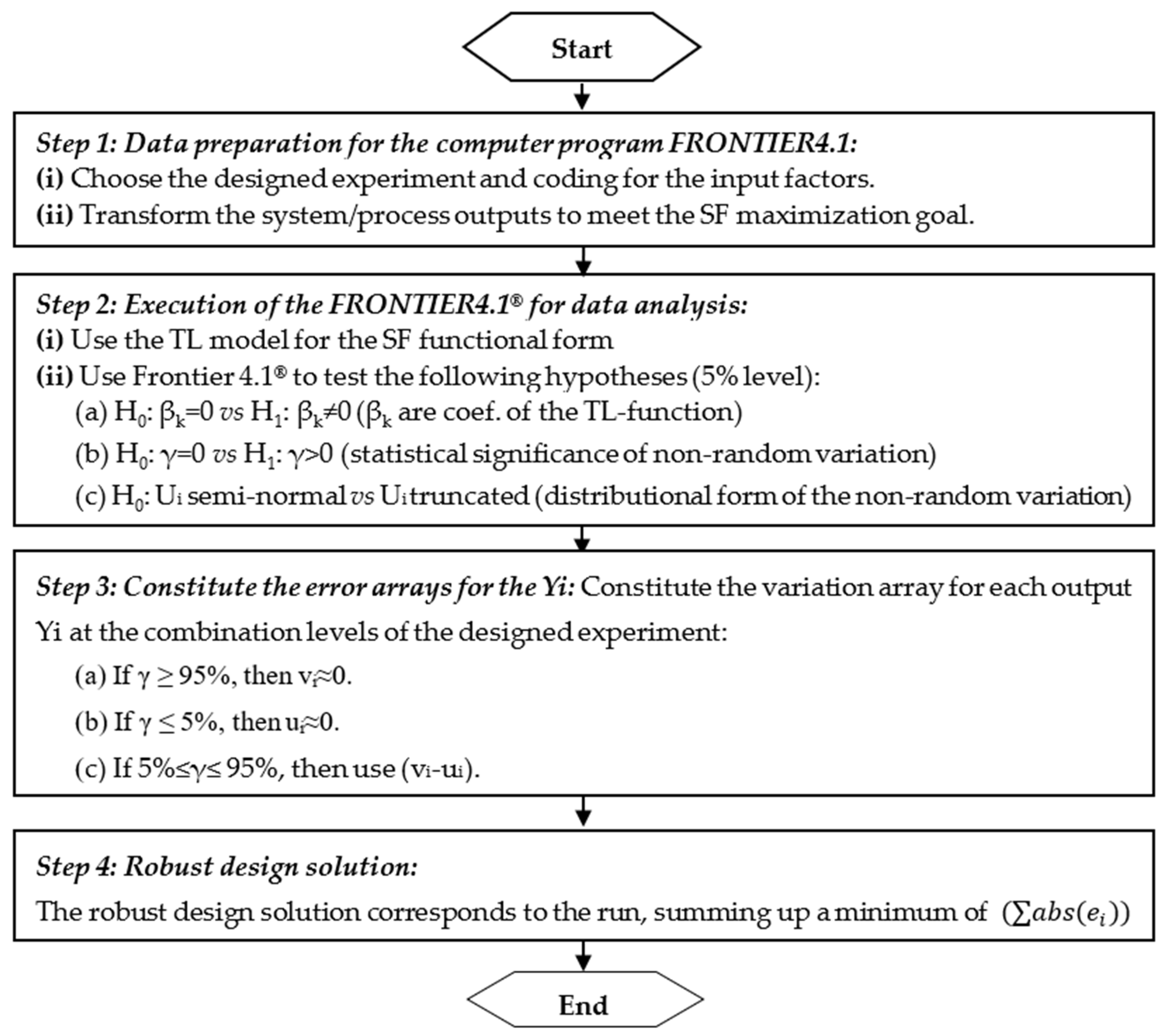
  • H0: βk = 0 vs. H1: βk ≠ 0. This is to check the statistical significance of the coefficients of the frontier model.
  • H0: γ = 0 vs. H1: γ > 0. This is to assess the fitness of the average line model (RSM) and investigate the statistical significance of the special cause error for the (Yi).
  • H0: Ui~Half-normal vs. H1: Ui~truncated normal distribution.
Only hypotheses (a) and (b) are checked for the RDPP-SF method [13,14]. The distributional form of the Ui is assumed to be half-normal.
Step 3, the printout, which is generated by the FRONTIER4.1® program, provides the regression model of the transfer function, the γ-value for each system response (Yi), and the inefficiency score of each run. The error array for Yi is based on the γ-value and the inefficiency score ui for each run (i). The ui(s) are obtained from the FRONTIER4.1® print output as the individual inefficiency (exp(-ui)).
  • If γ ≥ 95%, then vi ≈ 0 and special cause variation prevails. The error array (ei) is then composed of the ui(s) values of the output (Yi) for each run.
  • If γ ≤ 5%, then ui ≈ 0 and the bulk of variation is due to only random unit-to-unit variation. The error array (ei) is composed of the vi(s) values of the output (Yi) for each run. In this situation, the average line model (RMS) is confounding with the SF model.
  • If 5% ≤ γ ≤ 95%, both random and special cause variation sources are accountable for the result. The error array (ei) is then composed of the Abs(vi–ui) values of the output (Yi) for each run. The (vi–ui) values represent the observable variation in Yi.
Step 4 is concerned with lessening variation in each Yi for the multiple quality characteristics process. The least sensitive solution would correspond to the run (i*) in the designed experiment, which adds up to a minimum of ( abs ( e i ) ) accounting for all Yi(s).

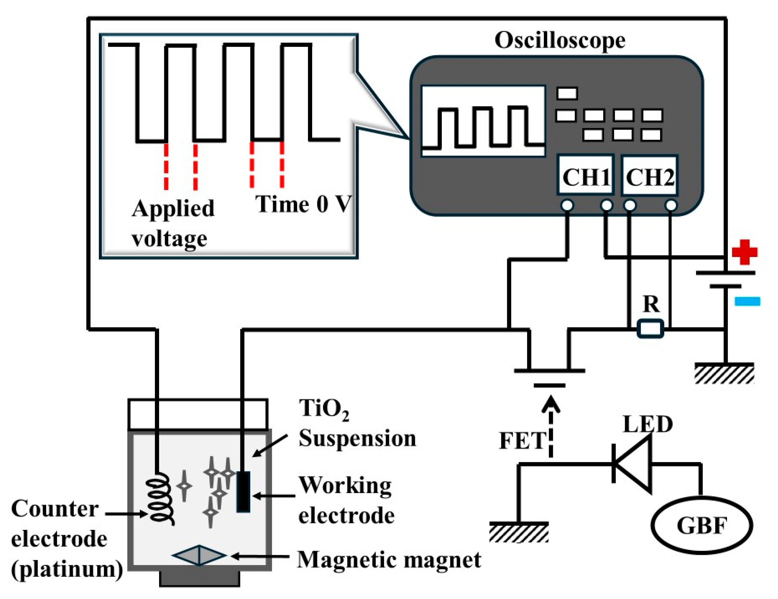
2. Materials and Methods

Barbana et al. [62] have conducted a central composite design (CCD) as an experimental strategy [63] to investigate the effects of four operating factors, i.e., the initial concentration (x1), the deposition time (x2), the duty cycle (x3), and the voltage (x3) on the properties of the TiO2 film. The levels of the operating factors (xi) are listed in Table 2. The SS-316L substrate preparation and pulsed electrophoretic deposition process are described in Barbana et al. [4]. Figure 2 shows the experimental coating process.
The process performance characteristics, i.e., De (photocatalytic efficiency of the thin film) and three critical charges, LC1, LC2, and LC3, are used to characterize the properties of the TiO2 films. LC1 is defined as the load at which the first cracks occurred (cohesive failure); LC2 is the load at which the film starts to delaminate at the edge level of the scratch track (adhesion failure); and LC3 is the load when the damage of the film exceeds 50%. The degradation experiments allow us to calculate the decolorization efficiency (De). All responses should be maximized. Table 3 shows the CCD layout as well as the process responses (De, LC1, LC2, and LC3). The 30 manipulations are prepared in random order for homogeneity.

3. Results and Discussion

The four steps listed above in Section 4 are followed when implementing the RDPP-SF method for static systems.
Step 1_ Data preparation: The data are arranged as required by the FRONTIER 4.1® program. Because the process outputs De, LC1, LC2, and LC3 are all larger-the-best types, no transformation is needed to satisfy the requirements of the stochastic frontier model.
Step 2_ Execution of FRONTIER 4.1® program and hypotheses testing: We choose a 5% type I error and a translog as a transfer function for the process responses. This choice is supported by the log-ratio values shown in Table 4 (tests 1); i.e., LR-stat = 37.98 for De, 50.94 for LC1, 48.92 for LC2, and 27.36 for LC3, respectively. The coefficients of the regression models for De, LC1, LC2, and LC3 are shown in Table 5.
Table 5 indicates that assuming a 5% error level, the γ-values for the LC1 and LC3 process responses are inferior to 5%, meaning that most of the residual variation is attributable to pure random sources of variation (sampling and part-to-part process variation). Therefore, the SF and neoclassic response surface model (RSM), are confounding. However, the high γ-values of 1 (at 3 dp) for the process outputs De and LC2 indicate that the bulk of variation is due to non-natural sources and that the SF and RSM are not confounding.
Step 3_ Constitute the error array for each process response (Yi): As for the γ-values, the abs(vi) terms at each run of the CCD layout make up the error arrays for the LC1 and LC3 outputs, while the ui values make up the error arrays for the De and LC2 outputs. Table 6 shows the error matrix for the De, LC1, LC2, and LC3 process responses.
Step 4_ Determination of the robust design solution: The error terms are added over the process responses for every run (i) in the CCD layout. The robust design solution corresponds to the one having a minimum value. Allowing for a 95% confidence interval, Table 6 and Figure 3 suggest that run 25 (initial concentration of 14 g/L, deposition time of 150 s, duty cycle of 50%, and voltage of 40 V) is the robust optimization setting for the pulsed electrophoretic deposition parameters on TiO2 film properties. Other potential design solutions, such as runs 23 and 29, should also be investigated based on their functionality, quality, and cost. Irrespectively, at a duty cycle of 50%, the voltage is the best sitting, which does not affect the sensitivity of the four outputs, De, LC1, LC2, and LC3. The level combinations of runs 24 and 30 yield the most sensitive design solutions, so they should be avoided at any cost.

4. Conclusions

The static RDPP-SF method was used for the robust design optimization of the electrophoretic deposition process on TiO2 films. The results of the hypothesis test regarding the residual variation in the De and LC2 responses show significance at the 5% level (both responses have a γ-value of one). Consequently, as the overall variation in the De and LC2 is not random, the EDP is not under statistical control concerning these outputs. Furthermore, the stochastic frontier and RSM are not confounding. From an output point of view of the stochastic production function, higher levels of De and LC2 outputs could be obtained while using the same input resources (xi). For the LC1 and LC3 outputs, the significance tests on non-random variation are insignificant at a 5% level (γ-values equals 0.05 and 0.00, respectively) meaning that the variation in the LC1 and LC3 process responses is only due to pure random sources (part-to-part variation). As a result, the least square response model (RSM) coincides with the stochastic frontier.
Table 6 shows the added values for the error arrays regarding the outputs De and the three critical charges LC1, LC2, and LC3. Accordingly, the robust optimization design for the pulsed electrophoretic deposition parameters corresponds to run 25 (minimum total). The robust optimization solution corresponds to the following setting: x1: initial concentration at 14 g/L; x2: deposition time at 150 s; x3: duty cycle at 50%; and x4: applied voltage at 40. Runs 23 and 29 are additional potential runs that should be accounted for from an economic standpoint. This study also showed that the duty cycle of 50% voltage is the best setting, which does not affect the sensitivity of the four outputs, De, LC1, LC2, and LC3 (see Table 6 and Table 7).
Using the response surface model (RSM) and desirability function method (RS-DF) as suggested in Barbana et al. [62], the optimum in continue space is obtained when setting the concentration of TiO2 at 16.34 g/L, the deposition time at 150 s, the duty cycle at 90%, and the applied voltage at 4 V. The discrepancy with the RDPP-SF method is partly due to the fact the RS-DF method [62] does not account for the non-random noise sources in the De% and LC2 responses. According to Table 7, pure non-natural variation (γ-value of nearly one) is present in both process responses. This suggests that contrary to Barbana et al. [62], the RSM should not be used to estimate the optimal setting for the De% and LC2 responses.
For the robust optimization of the EPD process, the RDPP-SF method can be viewed as a long-term reliability approach where part-to-part variation is compounded with non-natural sources of variation (noise variables). The objective is to engineer the process mean square deviation (MSD), which is associated with long-term process part-to-part, use, and deteriorative sources of variation.
The signal-to-noise metric, which is employed in many robust design techniques, can be linked with the RDPP-SF approach using the estimation of the γ-value metric. Thus, in engineering domains like reliability, resilience, adaptability, and versatility, the RDPP-SF approach has the greatest potential. However, the RDPP-SF method suffers from two major limitations: (i) A translog transfer function is used in the RDPP-SF method to consider the interactions between the control factors. Further investigation is required to identify alternative functional forms for engineering processes, and (ii) The RDPP-SF method uses graded rather than continued scales to code process parameters. An investigation utilizing a hybrid ANN-GA framework is being conducted to address the second limitation of the RDPP-SF approach.
Adopting optimized electrophoretic deposition (EPD) parameters in industrial settings offers substantial economic advantages. By refining these parameters, companies can achieve cost savings through enhanced process efficiency and minimized material wastage. Improved product quality resulting from optimized EPD parameters leads to heightened customer satisfaction and loyalty. Furthermore, the scalability of the process enables companies to handle larger production volumes without proportional increases in costs. Overall, these optimizations bolster industry competitiveness and profitability by streamlining operations and maximizing resource utilization.

Author Contributions

Conceptualization, A.T., M.A.R. and N.B.; methodology, A.T., M.A.R., N.B. and A.B.Y.; validation, N.B. and A.B.Y.; investigation, M.A.R. and N.B.; data curation, A.T. and N.B.; writing—original draft preparation, A.T., M.A.R. and N.B.; writing—review and editing, M.A.R., N.B. and M.A.-A. supervision, M.A.-A. All authors have read and agreed to the published version of the manuscript.

Funding

This research received no external funding.

Data Availability Statement

The data that support the findings of this study are available from the corresponding author (Nesrine Barbana) upon reasonable request.

Acknowledgments

We acknowledge support from the German Research Foundation and the Open Access Publication Fund of the Technical University of Berlin.

Conflicts of Interest

The authors declare no potential conflicts of interest concerning the research, authorship, and/or publication of this article.

References

  1. Zeribi, F.; Attaf, A.; Derbali, A.; Saidi, H.; Benmebrouk, L.; Aida, M.S.; Dahnoun, M.; Nouadji, R.; Ezzaouia, H. Dependence of the physical properties of titanium dioxide (TiO2) thin films grown by sol-gel (spin-coating) process on thickness. ECS J. Solid State Sci. Technol. 2022, 11, 023003. [Google Scholar] [CrossRef]
  2. Xu, J.; Nagasawa, H.; Kanezashi, M.; Tsuru, T. TiO2 coatings via atmospheric-pressure plasma-enhanced chemical vapor deposition for enhancing the UV-resistant properties of transparent plastics. ACS Omega 2021, 6, 1370–1377. [Google Scholar] [CrossRef]
  3. Puga, M.L.; Venturini, J.; Ten Caten, C.S.; Bergmann, C.P. Influencing parameters in the electrochemical anodization of TiO2 nanotubes: Systematic review and meta-analysis. Ceram. Int. 2022, 48, 19513–19526. [Google Scholar] [CrossRef]
  4. Barbana, N.; Ben Youssef, A.; Dhiflaoui, H.; Bousselmi, L. Preparation and characterization of photocatalytic TiO2 films on functionalized stainless steel. J. Mater. Sci. 2018, 53, 3341–3364. [Google Scholar] [CrossRef]
  5. Ben Youssef, A.; Barbana, N.; Al-Addous, M.; Bousselmi, L. Preparation and characterization of photocatalytic TiO2/WO3 films on functionalized stainless steel. J. Mater. Sci. Mater. Electron. 2018, 29, 19909–19922. [Google Scholar] [CrossRef]
  6. Santillán, M.; Membrives, F.; Quaranta, N.; Boccaccini, A. Characterization of TiO2 nanoparticle suspensions for electrophoretic deposition. J. Nanopart. Res. 2008, 10, 787–793. [Google Scholar] [CrossRef]
  7. Hanaor, D.; Michelazzi, M.; Veronesi, P.; Leonelli, C.; Romagnoli, M.; Sorrell, C. Anodic aqueous electrophoretic deposition of titanium dioxide using carboxylic acids as dispersing agents. J. Eur. Ceram. Soc. 2011, 31, 1041–1047. [Google Scholar] [CrossRef]
  8. de Sousa, R.R.M.; de Araújo, F.O.; da Costa, J.A.P.; Nishimoto, A.; Viana, B.C.; Alves, C., Jr. Deposition of TiO2 film on duplex stainless-steel substrate using the cathodic cage plasma technique. Mater. Res. 2016, 19, 1207–1212. [Google Scholar] [CrossRef]
  9. Gao, F.; Sherwood, P. Photoelectron spectroscopic studies of the formation of hydroxyapatite films on 316L. Surf. Interface Anal. 2012, 44, 1587–1600. [Google Scholar] [CrossRef]
  10. Krishna, D.; Chena, Y.; Sun, Z. Magnetron sputtered TiO2 films on a stainless-steel substrate: Selective rutile phase formation and its tribological and anti-corrosion performance. Thin Solid Films 2011, 519, 4860–4864. [Google Scholar] [CrossRef]
  11. Tang, F.; Uchikoshi, T.; Ozawa, K.; Sakka, Y. Effect of polyethyleneimine on the dispersion and electrophoretic deposition of nano-sized titania aqueous suspensions. J. Eur. Ceram. Soc. 2006, 26, 1555–1560. [Google Scholar] [CrossRef]
  12. Nurhayati, E.; Yang, H.; Chen, C.; Liu, C.; Juang, Y.; Huang, C.; Hu, C. Electro-photocatalytic fenton decolorization of orange G using mesoporous TiO2/stainless steel mesh photo-electrode prepared by the sol-gel dip-coating method. Int. J. Electrochem. Sci. 2016, 11, 3615–3632. [Google Scholar] [CrossRef]
  13. Trabelsi, A.; Rezgui, M.-A. Robust design of processes and products using the mathematics of the stochastic frontier. Int. J. Adv. Manuf. Technol. 2020, 106, 2829–2841. [Google Scholar] [CrossRef]
  14. Rezgui, M.-A.; Trabelsi, A. Use of the stochastic frontier and the grey relational analysis in robust design of multi-objective problems. Concurr. Eng. Res. Appl. 2020, 28, 110–129. [Google Scholar] [CrossRef]
  15. Taguchi, G. System of Experimental Design; UNIPUB/Kraus International Publications: White Plains, NY, USA, 1987. [Google Scholar]
  16. Del Castillo, E.; Montgomery, D.; McCarville, D.R. Modified desirability functions for multiple response optimization. J. Qual. Technol. 1996, 28, 337–345. [Google Scholar] [CrossRef]
  17. Chen, L.H. Designing robust products with multiple quality characteristics. Comput. Oper. Res. 1997, 24, 937–944. [Google Scholar] [CrossRef]
  18. Su, C.T.; Tong, L.I. Multi-response robust design by principal component analysis. Total Qual. Manag. 1997, 8, 409–416. [Google Scholar] [CrossRef]
  19. Tong, L.-I.; Su, C.T. Optimizing multi-response problems in the Taguchi method by fuzzy multiple attribute decision making. Qual. Reliab. Eng. Int. 1997, 13, 25–34. [Google Scholar] [CrossRef]
  20. Antony, J. Simultaneous optimization of multiple quality characteristics in manufacturing processes using Taguchi’s quality loss function. Int. J. Adv. Manuf. Technol. 2001, 17, 134–138. [Google Scholar] [CrossRef]
  21. Kim, K.J.; Lin, D.K.J. Simultaneous optimization of mechanical properties of steel by maximizing exponential desirability functions. J. R. Stat. Soc. Ser. C Appl. Stat. 2000, 49, 311–325. [Google Scholar] [CrossRef]
  22. Liao, H.-C.; Chen, Y.K. Optimizing multi-response problem in the Taguchi method by DEA-based ranking method. Int. J. Qual. Reliab. Manag. 2002, 19, 825–837. [Google Scholar] [CrossRef]
  23. Liao, H.-C. Using PCR-TOPSIS to optimize Taguchi’s multi-response problem. Int. J. Adv. Manuf. Technol. 2003, 22, 649–655. [Google Scholar] [CrossRef]
  24. Hsu, C.M.; Su, C.T.; Liao, D. Simultaneous of the broadband tap coupler optical performance based on neural networks and exponential desirability functions. Int. J. Adv. Manuf. Technol. 2004, 23, 896–902. [Google Scholar] [CrossRef]
  25. Ortiz, F.J.R.; Simpson, J.R.; Pignatiello, J.R.; Alejandro, H.L. A genetic algorithm approach to multiple-response optimization. J. Qual. Technol. 2004, 36, 432–449. [Google Scholar] [CrossRef]
  26. Liao, H.-C. Using N-D method to solve multi-response problem in Taguchi. J. Intell. Manuf. 2005, 16, 331–347. [Google Scholar] [CrossRef]
  27. Fung, C.P.; Kang, P.C. Multi-response optimization in friction properties of PBT composites using Taguchi method and principle component analysis. J. Mater. Process. Technol. 2005, 170, 602–610. [Google Scholar] [CrossRef]
  28. Liao, H.-C. Multi-response optimization using weighted principal component. Int. J. Adv. Manuf. Technol. 2006, 27, 720–725. [Google Scholar] [CrossRef]
  29. Liao, H.-C.; Chang, H.H.; Hsu, C.M. Using canonical correlation to optimize Taguchi’s multiresponse problem. Concurr. Eng. Res. Appl. 2006, 14, 141–149. [Google Scholar] [CrossRef]
  30. Köksoy, O.A. Nonlinear programming solution to robust multi-response quality problem. Appl. Math. Comput. 2008, 196, 603–612. [Google Scholar] [CrossRef]
  31. Al-Refaie, A. Grey-data envelopment analysis approach for solving the multi-response problem in the Taguchi method. Proc. IMechE Part B J. Eng. Manuf. 2010, 224, 147–158. [Google Scholar] [CrossRef]
  32. Pal, S.; Gauri, S.K. Multi-response optimization using multiple regression-based weighted signal-to-noise ratio (MRWSN). Qual. Eng. 2010, 22, 336–350. [Google Scholar] [CrossRef]
  33. Al-Refaie, A.; Rawabdeh, I.; Abu-Alhaj, R.; Jalham, I. A fuzzy multiple regressions approach for optimizing multiple responses in the Taguchi method. Int. J. Fuzzy Syst. Appl. 2012, 2, 13–34. [Google Scholar] [CrossRef]
  34. Canessa, E.; Bielenberg, G.; Allende, H. Robust design in multiobjective systems using Taguchi’s parameter design approach and Pareto genetic algorithm. Rev. Fac. Ing. Univ. Antioq. 2014, 72, 73–85. [Google Scholar] [CrossRef]
  35. Sylajakumari, P.A.; Ramakrishnasamy, R.; Palaniappan, G. Taguchi grey relational analysis for multi-response optimization of wear in co-continuous composite. Materials 2018, 11, 1743. [Google Scholar] [CrossRef] [PubMed]
  36. Sutono, S.B. Grey-based Taguchi method to optimize the multi-response design of product form design. J. Optimasi Sist. Ind. 2021, 20, 136–146. [Google Scholar] [CrossRef]
  37. Huang, W.-T.; Tasi, Z.-Y.; Ho, W.-H.; Chou, J.-H. Integrating Taguchi method and gray relational analysis for auto locks by using multiobjective design in computer-aided engineering. Polymers 2022, 14, 644. [Google Scholar] [CrossRef]
  38. Muthana, S.A.; Ku-Mahamud, K.R. Taguchi-Grey relational analysis method for parameter tuning of multi-objective pareto ant colony system algorithm. J. Inf. Commun. Technol. 2023, 22, 149–181. [Google Scholar] [CrossRef]
  39. Parinam, S.; Kumar, M.; Kumari, N.; Karar, V.; Sharma, A.L. An improved optical parameter optimisation approach using taguchi and genetic algorithm for high transmission optical filter design. Optik 2019, 182, 382–392. [Google Scholar] [CrossRef]
  40. Parnianifard, A.; Azfanizam, A.S.; Ariffin, M.K.A.; Ismail, M.I.S. Trade-off in robustness, cost and performance by a multi-objective robust production optimization method. Int. J. Ind. Eng. Comput. 2019, 10, 133–148. [Google Scholar] [CrossRef]
  41. Viswanathan, R.; Ramesh, S.; Maniraj, S.; Subburam, V. Measurement and Multiresponse Optimization of Turning Parameters for Magnesium Alloy Using Hybrid Combination of Taguchi GRA- PCA Technique. Measurement 2020, 159, 107800. [Google Scholar] [CrossRef]
  42. Sreedharan, J.; Jeevanantham, A.K.; Rajeshkannan, A. Multi-objective optimization for multi-stage sequential plastic injection molding with plating process using RSM and PCA-based weighted-GRA. Proc. Inst. Mech. Eng. Part C J. Mech. Eng. Sci. 2020, 234, 1014–1030. [Google Scholar] [CrossRef]
  43. Kumar, D.; Mondal, M. Process parameters optimization of AISI M2 steel in EDM using Taguchi based TOPSIS and GRA. Mater. Today-Proc. 2020, 26, 2477–2484. [Google Scholar] [CrossRef]
  44. Li, Y.; Zhu, L. Multi-objective optimisation of user experience in mobile application design via a grey-fuzzy-based Taguchi approach. Concurr. Eng.-Res. A 2020, 28, 175–188. [Google Scholar] [CrossRef]
  45. Huang, W.-T.; Tsai, C.-L.; Ho, W.-H.; Chou, J.-H. Application of intelligent modeling method to optimize the multiple quality characteristics of the injection molding process of automobile lock parts. Polymers 2021, 13, 2515. [Google Scholar] [CrossRef]
  46. Lin, C.-M.; Hung, Y.-T.; Tan, C.-M. Hybrid Taguchi–gray relation analysis method for design of metal powder injection-molded artificial knee joints with optimal powder concentration and volume shrinkage. Polymers 2021, 13, 865. [Google Scholar] [CrossRef]
  47. Jiang, R.; Zou, B. A DEA-based multi-response fusion model in the context of Taguchi method. In Proceedings of the Fourth International Conference on Mechanical, Electric and Industrial Engineering, Kunming, China, 22–24 May 2021; Volume 1983, p. 012108. [Google Scholar]
  48. Tanash, M.; Al Athamneh, R.; Bani Hani, D.; Rababah, M.; Albataineh, Z. A PDCA framework towards a multi-response optimization of process parameters based on Taguchi-fuzzy model. Processes 2022, 10, 1894. [Google Scholar] [CrossRef]
  49. Li, J.; Horber, D.; Keller, C.; Grauberger, P.; Goetz, S.; Wartzack, S.; Matthiesen, S. Utilizing the embodiment function relation and tolerance model for robust concept design. In Proceedings of the International Conference On Engineering Design, ICED23, Bordeaux, France, 24–28 July 2023. [Google Scholar]
  50. Chen, L.; Rottmayer, J.; Kusch, L.; Gauger, N.R.; Ye, Y. Data-driven aerodynamic shape design with distributionally robust optimization approaches. arXiv 2023, arXiv:2310.08931v1. [Google Scholar]
  51. Shrimali, R.; Kumar, M.; Pandey, S.; Sharma, V.; Kaushik, L.; Singh, K. A robust Taguchi combined AHP approach for optimizing AISI1023 low carbon steel weldments in the SAW process. Int. J. Interact. Des. Manuf. 2023, 17, 1959–1977. [Google Scholar] [CrossRef]
  52. Zheng, M.; Teng, H.; Wang, Y. Application of new robust design by means of probability-based multi-objective optimization to machining process parameters. Vojnoteh. Glas. Mil. Tech. Cour. 2023, 71, 84–99. [Google Scholar] [CrossRef]
  53. Zheng, M.; Yu, J. Probabilistic approach for robust design with orthogonal experimental methodology in case of target the best. J. Umm Al-Qura Univ. Eng. Archit. 2024, 15, 55–59. [Google Scholar] [CrossRef]
  54. Parnianifard, A.; Azfanizam, A.S.; Ariffin, M.K.A.; Ismail, M.I.S. An overview on robust design hybrid metamodeling: Advanced methodology in process optimization under uncertainty. Int. J. Ind. Eng. Comput. 2018, 9, 1–32. [Google Scholar] [CrossRef]
  55. Coelli, J.T.; Rao, P.; Christopher, O.J.; Battese, E.G. An Introduction to Efficiency and Productivity Analysis, 2nd ed.; Springer: New York, NY, USA, 2005. [Google Scholar]
  56. Aigner, D.; Knox Lovell, C.A.; Peter, S. Formulation and estimation of stochastic frontier production function models. J. Econ. 1977, 6, 21–37. [Google Scholar] [CrossRef]
  57. Meeusen, W.; Van Den Broeck, J. Efficiency estimation from Cobb–Douglas production functions with composed error. Int. Econ. Rev. 1977, 18, 435–444. [Google Scholar] [CrossRef]
  58. Schmidt, P.; Knox Lovell, C.A. Estimating stochastic production and cost frontiers when technical and allocative inefficiency are correlated. J. Econ. 1980, 13, 83–100. [Google Scholar] [CrossRef]
  59. Von Hirschhausen, C.R.; Cullmann, A.; Kappeler, A. Efficiency analysis of German electricity distribution utilities–non–parametric and parametric tests. Appl. Econ. 2006, 38, 2553–2566. [Google Scholar] [CrossRef]
  60. Montgomery, D.C. Design and Analysis of Experiments, 9th ed.; John Wiley & Sons, Inc.: Hoboken, NJ, USA; Arizona State University: Tempe, AZ, USA, 2017; p. 749. [Google Scholar]
  61. Coelli, J.T. A Guide to FRONTIER Version 4.1: A Computer Program for Stochastic Frontier Production and Cost Function Estimation; Centre for Efficiency and Productivity Analysis, University of New England: Armidale, Australia, 1996. [Google Scholar]
  62. Barbana, N.; Ben Youssef, A.; Rezgui, M.-A.; Bousselmi, L.; Al-Addous, M. Modelling, analysis, and optimization of the effects of pulsed electrophoretic deposition parameters on TiO2 films properties using desirability optimization methodology. Materials 2020, 13, 5160. [Google Scholar] [CrossRef]
  63. Box, G.E.P.; Wilson, K.B. On the experimental attainment of optimum conditions. J. R. Stat. Soc. Ser. B 1951, 13, 1–45. [Google Scholar] [CrossRef]
Figure 1. Functional scheme for the static multi-objective RDPP-SF method.
Inventions 09 00031 g001
Figure 2. Schematic illustration of a pulse circuit generator and working electrophoresis cell [4].
Inventions 09 00031 g002
Figure 3. Global error values at each run of the CCD plan.
Inventions 09 00031 g003
Table 1. Mapping table econometric—RDPP-SF.
Econometric ModelRDPP-SF MethodPerformance Metric
DMUsDesign plan (DoE) γ = σ u 2 σ v 2 + σ u 2
DMUiExecution i in the DoE
Cross/panel dataNonreplicated/replicated
vi: Random variationNatural noise (experimental and unit-to-unit variation)
ui: TENon-natural noise (environment and degradation)
Table 2. The setting of the engineering factors’ levels used in the CCD plan.
Operating FactorsUnitsLevels
α−10+1+α
x1: Initial concentrationg/L28142026
x2: Deposition times150300450600750
x3: Duty cycle (DC)%1030507090
x4: VoltageV422405876
Table 3. CCD layout for the experimental study.
RunOperating Parameters (Coded Values)Performance Characteristics (PCHs)
x1 (g/L)x2 (s)x3 (%)x4 (V)De (%)LC1 (N)LC2 (N)LC3 (N)
1−1−1−1−176.394.698.889.23
21−1−1−183.573.897.569.56
3−11−1−168.774.677.3210.74
411−1−158.872.326.8913.84
5−1−11−157.584.789.2911.21
61−11−161.963.247.5211.47
7−111−131.825.1910.0510.78
8111−129.232.926.5912.85
9−1−1−1130.963.616.539.64
101−1−1138.364.397.948.96
11−11−1143.902.565.3210.92
1211−1141.683.256.3610.45
13−1−11142.262.975.5111.85
141−11150.093.806.259.35
15−111134.422.944.4810.30
16111134.622.754.3510.26
17000052.093.466.359.56
18000051.893.567.349.17
19000050.573.556.149.75
20000053.243.876.719.64
21000055.093.525.989.43
22000051.843.776.859.58
23−α00036.133.505.268.41
2400035.522.604.978.53
250−α0060.965.898.929.30
2600041.313.966.4410.33
2700−α070.953.246.9210.45
2800045.373.066.91111.94
29000−α57.624.869.9614.46
3000024.562.925.9812.05
Table 4. Hypotheses tests on the SF models for the De, LC1, LC2, and LC3 PCHs outputs.
Hypotheses (α = 5%)LR-stat.χ20.95-ValueDecision
DeTest 1Linear vs. quadratic37.9818.31Reject
Test 2γ = 013.672.71Reject
LC1Test 1Linear vs. quadratic50.9418.31Reject
Test 2γ = 00.002.71Fail to Reject
LC2Test 1Linear vs. quadratic.48.9218.31Reject
Test 2γ = 042.402.71Reject
LC3Test 1Linear vs. quadratic.27.3618.31Reject
Test 2γ = 00.002.71Fail to reject
Table 5. Estimates of the SF models for De, LC1, LC2, and LC3 outputs.
VariablesParam.De(%)
(γ ≠ 0; µ = η = 0)
LC1(N)
(γ ≠ 0; µ = η = 0)
LC2(N)
(γ = 0, OLS)
LC3(N)
(γ = 0, OLS)
Est.t-test.Est.t-test.Est.t-test.Est.t-test.
Cte.β0−1.244−1.26914.01614.016−4.1854.280−3.7771.579
ln(x1)β12.4092.578 *0.7030.7030.6850.730−0.019−0.026
ln(x2)β24.0706.575 *−3.508−3.508 *0.5781.0820.3850.586
ln(x3)β31.6791.981−0.613−0.6131.4191.6451.5121.719
ln(x4)β4−6.007−6.858 *−0.284−0.2841.1391.3780.8751.321
ln(x1)^2β5−0.153−3.602 *−0.098−0.098−0.141−4.960 *−0.072−2.536
ln(x1)*ln(x2)β6−0.294−1.804−0.373−0.373−0.092−0.7580.2342.267
ln(x1)*ln(x3)β70.0100.061−0.138−0.138−0.230−2.259 *−0.063−0.763
ln(x1)*ln(x4)β80.0200.1380.6640.6640.3834.390*−0.224−3.027
ln(x2)^2β9−0.290−3.644 *0.2790.279−0.011−0.1960.0631.014
ln(x2)*Ln(x3)β10−0.670−5.869 *0.3620.3620.0550.430−0.315−2.706
ln(x2)*Ln(x4)β110.6664.660 *−0.144−0.144−0.166−1.549−0.114−1.215
ln(x3)^2β12−0.047−1.110−0.080−0.080−0.031−0.7240.0842.152
ln(x3)*ln(x4)β130.6824.155 *−0.185−0.185−0.258−2.916 *0.0020.027
ln(x4)^2β14−0.159−4.281 *−0.002−0.002−0.055−2.265 *0.0462.161
σ 2 = σ v 2 + σ u 2 0.030.0050.0120.005
γ-value1.0000.051.0000.000
µ, η----
Log (likelihood)31.7936.4842.4038.44
Critical t-value (5%) = 1.753
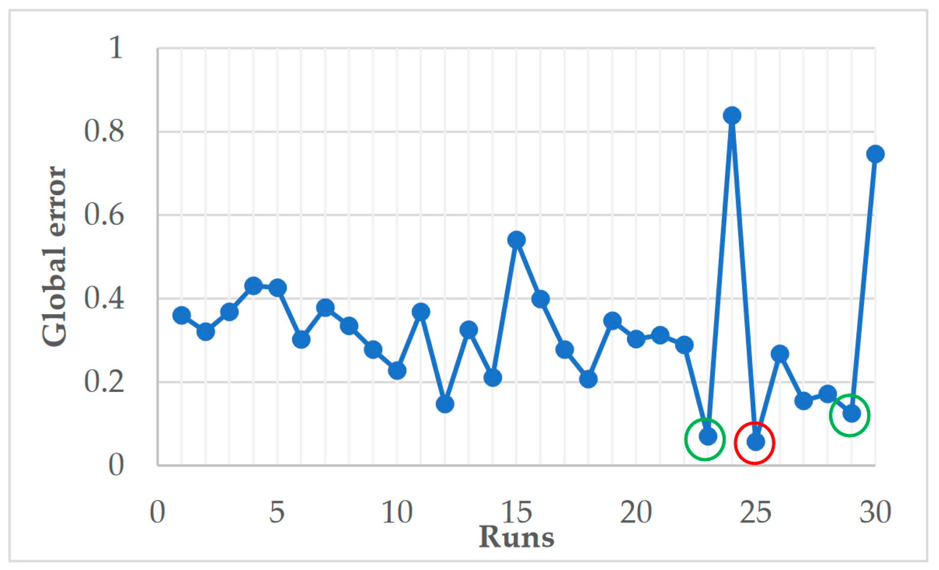
* Starred coefficients are significant parameters at a 5% level.
Table 6. Global error table for the De, LC1, LC2, and LC3 outputs.
RunOperating FactorsPCHsGlobal ErrorRanking
x1 (g/L)x2 (s)x3 (%)x4 (V)De(%)LC1(N)LC2(N)LC3(N)
uiAbs(vi)uiAbs(vi)
1830030220.2530.0660.0040.0380.36021
22030030220.2090.0550.0210.0360.32117
3860030220.1710.0140.1440.0400.36823
42060030220.1850.1360.0020.1080.43127
5830070220.2200.0320.1430.0320.42626
62030070220.1990.0040.0320.0670.30214
7860070220.2320.0760.0430.0280.37924
82060070220.1830.0010.0840.0670.33519
9830030580.2020.0250.0400.0110.27811
102030030580.0500.0590.0410.0780.2289
11860030580.1130.1340.0810.0400.36822
122060030580.0410.0570.0400.0100.1484
13830070580.1340.0020.1820.0070.32618
142030070580.0350.0700.0740.0330.2118
15860070580.2060.0430.2570.0350.54128
162060070580.0840.0460.2450.0230.39925
171445050400.0560.0120.1450.0650.27812
181445050400.0600.0400.0000.1070.2077
191445050400.0860.0370.1790.0460.34720
201445050400.0340.1220.0900.0570.30315
211445050400.0000.0290.2050.0790.31316
221445050400.0610.0960.0690.0630.28913
23245050400.0050.0400.0160.0100.0702
242645050400.3280.1210.2670.1230.83930
251415050400.0030.0110.0120.0320.0571
261475050400.0010.1730.0250.0680.26810
271445010400.0130.0360.0570.0500.1555
281445090400.0370.0390.0210.0750.1726
29144505040.0140.0250.0420.0440.1253
301445050760.4910.0620.0050.1890.74729
Table 7. Optimization results of RDPP-SF [13,14] vs. RS-DF [62] methods.
Operating FactorsProcess Responses
x1 (g/L)x2 (s)x3 (%)x4 (V)De (%)LC1 (N)LC2 (N)LC3 (N)
γ-Value----1.0000.0501.0000.000
RDPP-SFrun 2514150504060.9605.8908.9209.300
run 232450504036.1303.5005.2608.410
run 291445050457.6204.8609.96014.460
RSM-Desirability [41] method16.3415090482.7575.89512.58416.773
Disclaimer/Publisher’s Note: The statements, opinions and data contained in all publications are solely those of the individual author(s) and contributor(s) and not of MDPI and/or the editor(s). MDPI and/or the editor(s) disclaim responsibility for any injury to people or property resulting from any ideas, methods, instructions or products referred to in the content.

