
Silencer Design for the Control of Low Frequency Noise in Ventilation Ducts
by
 , ,
, ,
Edoardo Alessio Piana
1,* ,
,
Ulf Erik Carlsson
2, 
Adriano Maria Lezzi
3,
Diego Paderno
3 and
Susann Boij
2 1
Applied Acoustics Laboratory, University of Brescia, Via Branze 38, 25123 Brescia, Italy
2
MWL, Department of Engineering Mechanics, KTH—Royal Institute of Technology, Teknikringen 8, SE-100 44 Stockholm, Sweden
3
Department of Mechanical and Industrial Engineering, University of Brescia, Via Branze 38, 25123 Brescia, Italy
*
Author to whom correspondence should be addressed.
Designs 2022, 6(2), 37; https://doi.org/10.3390/designs6020037
Submission received: 17 February 2022
/
Revised: 18 March 2022
/
Accepted: 4 April 2022
/
Published: 6 April 2022
(This article belongs to the Special Issue Sustainable and Conventional Buildings)
Abstract
:The control of noise propagating along ventilation system ducts has always been an important issue in the building and vehicle sectors. This problem is generally tackled by selecting noise-reducing components with a suitable transmission loss, possibly verifying their effectiveness at a later time. The aim of this article is to characterize the nature of the problem and propose a design approach focusing directly on the perceived effect, that is, on the sound pressure level downstream of the outlet. Because the nature of the noise emission depends on various generation mechanisms, different methods can be applied. Usually, it is more difficult to realize good attenuations at low frequencies because of the limits of sound absorbing materials in such frequency range. For this reason, the ability of reactive components to attenuate the noise below the cut-on frequency will be investigated. This goal is reached by applying the transfer matrix approach to a duct system, with the implementation of the transfer matrices of each single element, and then assembling a system capable of acoustically describing the source and the duct structure. The coupling between the duct system with source and receiver impedances allows one to predict the sound pressure level at a given distance from the outlet. The proposed methodology is implemented in a user-friendly calculation tool with possible academic and professional application. Predictive capability, usability, and intuitiveness of the proposed design procedure are validated against experimental results by real potential users, who express positive feedback.
1. Introduction
The control of noise in duct systems is a topic of interest in many different sectors. All ducts through which gas flows generate acoustic noise. Sometimes the generated noise causes too high noise exposure or discomfort for operators, drivers, passengers, etc. In such cases, adequate noise reduction measures must be taken. Some examples are vehicles [1,2,3,4,5], buildings [6,7], ships [8,9,10], industries [11,12], and energy plants [13,14,15,16].
Choosing suitable noise reduction measures requires expert knowledge on how the noise is generated and transmitted from the sources to the observation point. Normally, the duct flow noise contains both tonal and random components. The random components, caused by turbulent flow, are distributed over a wide frequency range, whereas the tonal components appear at distinct frequencies. Tonal components are caused by periodic processes or phenomena such as ones involving fans [17,18,19,20] or compressors [7,21,22] running at constant speed or periodic eddy generation [23,24] causing whistling noises. From a noise comfort point of view the tonal components cause more discomfort than the wide-band turbulence flow noise. Therefore, the noise reduction measures often focus on the tonal components. After a comparison of the problematic frequencies with the characteristics of the possible generation mechanisms, the source causing problems can be identified. Once the sources have been identified, it is possible to choose how to reduce the noise, working on the source generation mechanism or on the transmission via the duct.
This type of problem is assuming an ever-growing interest with the expansion of heat recovery ventilation systems. Indeed, the comfort inside buildings is a particularly challenging issue given the extremely low background noise that can be found in some very quiet environments [25,26]. For the same reason, it is important to properly design the building elements against tapping noise, especially for lightweight structures [27]. because many solutions can also be used for façade sound insulation, the thermal properties of classic and sustainable materials can also be of interest [28,29].
As concerns the design of silencers suitable for reducing tonal noise transmitted along the duct system, there are two fundamentally different types of elements: resistive, based on acoustic energy dissipation, and reactive, based on wave interference. Typical resistive elements are porous materials, orifices, and perforated plates. Recently, micro-perforated plates and 3D printed porous materials have becoming more widely used in the aerospace industry because their acoustic properties can be easily tuned to obtain high performance silencers working at specific frequencies or over a broad band frequency range. Another technique used to reduce noise in ducts is based on active control. Even if it is very interesting and a subject of a number of scientific publications, this type of sound reduction strategy will not be considered in this paper because it requires additional electronic components (DSP microphones and actuators), which make it expensive to apply in real cases. In contrast to most of the resistive elements, reactive silencer elements can be tuned to have very high noise reduction capabilities at specific frequencies. Hence, reactive elements are the natural choice for the reduction of low frequency tonal noise.
An interesting way to describe a system through an electro-acoustic analogy was introduced by Schönfeld [30]. The main advantage is the ability of the method to describe the elements through a lumped parameters approach, thus allowing an easy implementation and fast calculations. Later, this theory was mainly applied to exhaust systems. The approach requires the characterization of the source and of the outlet impedances. A contribution to the modelling of fluid machines as sources of sound in duct and pipe systems is given in [31]. Later, Glav and Åbom developed a general formalism for analyzing acoustic two-port networks [32]. Such work led to the realization of lumped parameters software for simulating the sound propagation in complex duct systems based on the transfer matrix method [33]. This paper shows how the transfer matrix method can be used to design reactive silencers suitable for solving the specific noise problem at hand. It is interesting to note that the transfer matrix approach can also be adopted for the acoustic design of building elements, as shown by Caniato [34].
One positive property of the transfer matrix method, also known as the T-matrix method or TMM, is that it describes each silencer element with its T-matrix, and the complete silencer properties can be easily obtained by a combination of the elements’ T-matrices [35].
In particular, the overall sound transmission loss (TL) can be obtained as a direct out-put of the model. The general approach is, therefore, to estimate the TL required to fulfill the design specifications and to select and combine components that can provide it while respecting some practical constraints, such as cost and size limits. However, this approach does not return the impact of the solution on the perceived noise, leaving this verification to a later time. In recent years, comfort evaluations are gradually moving towards an occupant-centric paradigm, which involves the adaptation of traditional design methods to more detailed, easy-to-interpret approaches.
This paper fills the gap by proposing an expanded TMM method (xTMM), integrating the classic TMM procedure to build a reactive silencer with the possibility to evaluate its effectiveness directly in terms of perceived noise—namely, sound pressure level at a certain distance from the ductwork outlet. A self-developed tool in MATLAB is also described that can be used in academic and professional courses to promote noise-oriented design approaches.
The paper presents the formulation of noise in ducts in Section 2. Section 3 describes the xTMM method, based upon coupling the TMM system with source and receiver impedances, and introduces the self-developed design tool and its characteristic components. Section 4 presents the procedure adopted in the design stage. Section 5 discusses the case study, and finally Section 6 draws the conclusions.
2. Noise Generation and Propagation in Ducts
There are different generation mechanisms that build up noise in ducts. Some of them are related to rotating machinery or vibrating membranes, some others have a fluid-dynamic origin such as vortex shedding and turbulence. Usually, once the noise is generated by a source, it propagates inside the duct until it is radiated by an outlet. In the case of ventilation systems, noise is caused by two main sources: a fan or a compressor and the turbulence generated by the air flow in the ducts [36]. At constant speed, the ventilation system fan drives an air volume flow through the ventilation ducts. The volume flow has a non-zero mean value and a superimposed pulsating part caused by the fan blades. At constant speed, the pulsating part causes a tonal acoustic noise. The mean flow itself generates a wide-band random character noise caused by turbulent vortex shedding in the boundary layer between the air flow and the duct walls, and at the fan blades. At specific flow conditions, some components can generate a whistling noise. All these sound generating mechanisms cause volume flow disturbances that radiate acoustic noise from the duct outlet to the receiving environment.
The cut-on frequency is the frequency below which only plane waves propagate in the duct. For example, in a circular duct such frequency is defined as:
where c is the speed of sound in the duct and D is the duct diameter. Above the cut-on frequency, the shape of the wave front is no longer plane, and a good attenuation can be easily achieved by placing absorbing material on the duct walls [37]. For this reason, an advanced design procedure is not necessary to reduce noise components above the cut-on frequency. The cut-on frequency discriminates the low-frequency range from the high-frequency range and gives a first numerical indication on the frequency interval where an acoustic design based on the plane wave assumption is feasible. Below the cut-on frequency, alternative methods must be applied to reduce the noise. Such methods refer to the use of reactive elements, which must be designed to reflect a part of the sound wave with an opposite phase with respect to the sound propagating in the duct. To have such an effect, an abrupt change in the impedance characteristics of the duct is necessary. There are different reactive elements able to introduce an impedance change that can be used to achieve a reduction of the noise at the outlet, and they are: area discontinuities, expansion chambers, and side branches. Each one of these elements has a different behavior that can be exploited to build a system w a broad band sound attenuation. An overview of the devices that can be used for the acoustic design is given in the following sections.
Reactive elements are effectively used to attenuate noise in specific frequency ranges, generally related to the motor rpm and number of blades of a fan [37]. The “passing by frequency” can be computed as:
where rpm is the number of revolutions per minute of the motor and bn is the number of blades of the fan. This is the lowest frequency at which an attenuation may be required. Higher-order harmonics can be computed as:
where n is a natural number. Usually, the first two harmonics (n = 2, 3) correspond to the loudest components, which are the target when designing reactive elements.
The amount of attenuation given by a duct element is usually expressed using two different descriptors: transmission loss (TL) and insertion loss (IL). The TL is defined as the acoustical power difference between the forward travelling incident pressure wave at the inlet of the element and the forward travelling transmitted pressure wave at the outlet of the element. Expressed in decibels, the equation for determining the TL reads:
where W is the sound power, p is the sound pressure, S is the cross section, and the “in” and “out” subscripts indicate the inlet and the outlet of the considered element, respectively.
The IL is defined as twenty times the logarithm of the pressure measured at a certain point in two different system configurations a and b:
As an example, for regulatory applications concerning vehicle noise, the IL is used to compare the sound pressure level (SPL) at 1 m distance, 45° from the outlet of an exhaust system without a silencer to the SPL in the same position when a silencer is fitted on the exhaust system. From a practical point of view, the IL is usually the easiest and most common way for evaluating the sound reduction properties of a silencer system. However, this may not be enough to ensure acceptable conditions in some practical situations, such as the assessment of acoustic comfort in indoor environments with mechanical ventilation systems. In such cases, the SPL in a given position must be estimated, which requires the knowledge of quantities such as source impedance, the nature of the ground (reflection coefficient), and the radiation model of the outlet [38,39].
3. Silencer Design with xTMM
3.1. Overview
The proposed design method is based on a scientific approach. More specifically, the lumped parameters acoustic modeling is positioned halfway between a purely empirical approach and the application of computationally burdensome FEM or BEM simulations. Nevertheless, this method holds some of the attractive features of both approaches, such as quick implementation, short calculation time [40], and consistency with experimental results [41]. A method based on the same element model has been used recently for designing the exhaust systems of vehicles [42] as well as many other systems [43,44,45,46]. The method can also be adapted to be used outside the automotive field, for example to design industrial mufflers as well as HVAC ducts or thermal recovery ventilation systems, with the fire frequency replaced by the blade passing frequency of fans generating noise.
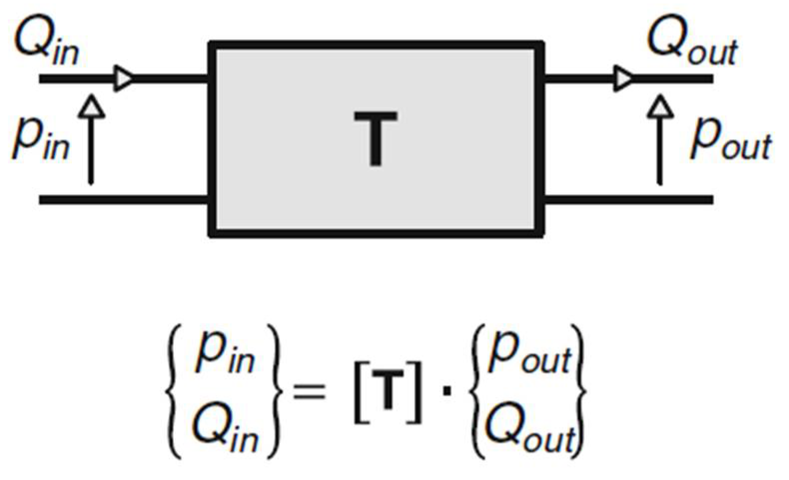
In this approach, the duct is split into fundamental blocks, each one having an inlet and an outlet. Such blocks can be characterized by different transfer matrices relating two variables: the sound pressure, p, and the volumetric flow rate, Q. Applying an electro-acoustic analogy where the pressure is equivalent to voltage and the volumetric flow to current, the transfer matrix approach can be considered as the equivalent of the two Kirchhoff’s circuit laws. The interconnection of different blocks can be expressed by a product of the different transfer matrices characterizing the single blocks describing the system (Figure 1).
Under linear conditions, the T-matrix method can be used to describe the acoustic properties of a silencer system. All models described hereafter assume 1-dimensional plane wave propagation along the duct axis. This means that the models are valid up to a higher frequency limit where the cross section is small compared to half a wavelength. Each block corresponds to a physical component and has a specific effect on the overall sound attenuation of the system. Detailed references to the mathematical models of the single elements described hereafter can be found in [36]. The selection of these blocks and the ability to simulate their combined effect is therefore the key to a good acoustic design of the system.
In this work, a software developed in MATLAB has been used to perform the simulations. Below the cut-on frequency, the software can model the system as a network of blocks because the continuous field variables describing pressure or volumetric flow variations (p(x,t) and Q(x,t)) in the real system can be discretized into elements in which one of the quantities can be assumed to be a locally spatially invariant (p(t) and Q(t)) [36].
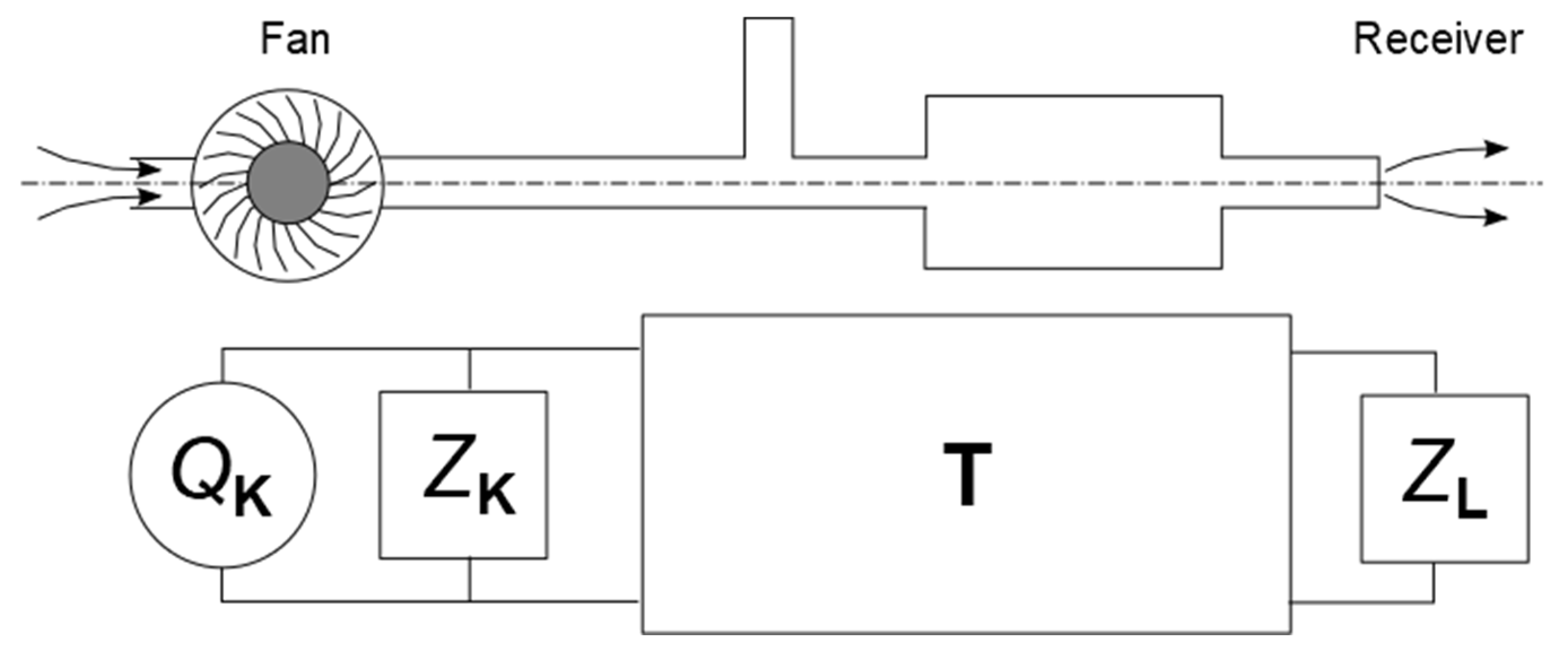
The elements can be selected among several pre-determined elements. These elements are the most common reactive devices used to attenuate low frequency noise and will be introduced in the next section. Figure 2 gives an example of a complete ventilation system and its acoustic T-matrix model. The T-matrix method is tailored for analysis of cascade-coupled systems. The overall behavior can be described by a “total” T-matrix equal to the product of the single T-matrices of its constituents:
The transmission loss of a silencer is a measure of the isolated silencer noise reduction capacity. It is a useful tool when a silencer component is tuned to a certain problematic frequency or frequency range. The insertion loss, on the other hand, also accounts for the system source and receiver impedances. Hence, it is ideal as a measure of the capability of a silencer to reduce the noise when it is installed in the system.
The system transmission loss, expressed using the duct system T-matrix components and the impedances at the duct inlet and outlet, is:
where tij are elements of the system T-matrix. If the impedances at the inlet (Zin) and outlet (Zout) are equal to the corresponding duct plane wave specific impedance, ⍴0c/Sin and ⍴0c/Sout, respectively, reflection free in- and outlets have been assumed. Using this assumption, it is possible to analyze the system sound reduction properties without any influence from the source and the receiver impedances.
The insertion loss, expressed in terms of the system acoustic properties, is:
where tij and tr,ij are T-matrix elements for the case ”with” silencer and the reference case “without” silencer, respectively.
In the construction and validation phases, a silencer system was built and its insertion loss measured. The measured insertion loss could be used to compare and validate the predicted insertion loss. A relevant comparison requires a good estimation of the source and receiver impedances, ZK and ZL. In the MATLAB scripts, the receiver properties are described with the “free space” impedance model, while the source impedance is described with the impedance measured on the loudspeaker used during the validation measurements.
It is worth noting that the xTMM method retains the same limitations of the classic TMM, in that:
- it is only valid under the duct cut-on frequency;
- because it is applicable in the plane wave range, the results are not valid in the vicinity of acoustic treatments or close to duct shape or size variations;
- it neglects evanescent coupling between the silencer elements [47];
- In the following, the reactive elements that can be combined to design the silencer are briefly recalled, based on the formulae in [36]. The time dependence adopted in this work is exp(iωt). As shown in the following Section 3.2.3, such an assumption helps to remove discontinuities (infinity points) to the TL computed for quarter-wavelength resonators. In the case of particularly narrow ducts, Stinson’s model [48] can also be applied. The transmission loss plots in Section 3.2 refer to the actual elements used for the experiments in Section 5. Components are assumed to be characterized by an internal friction factor, Xi, which can be used to estimate pressure drops (see Section 3.3).
3.2. T-Matrices for Acoustical-Physical Elements
3.2.1. Straight Pipe
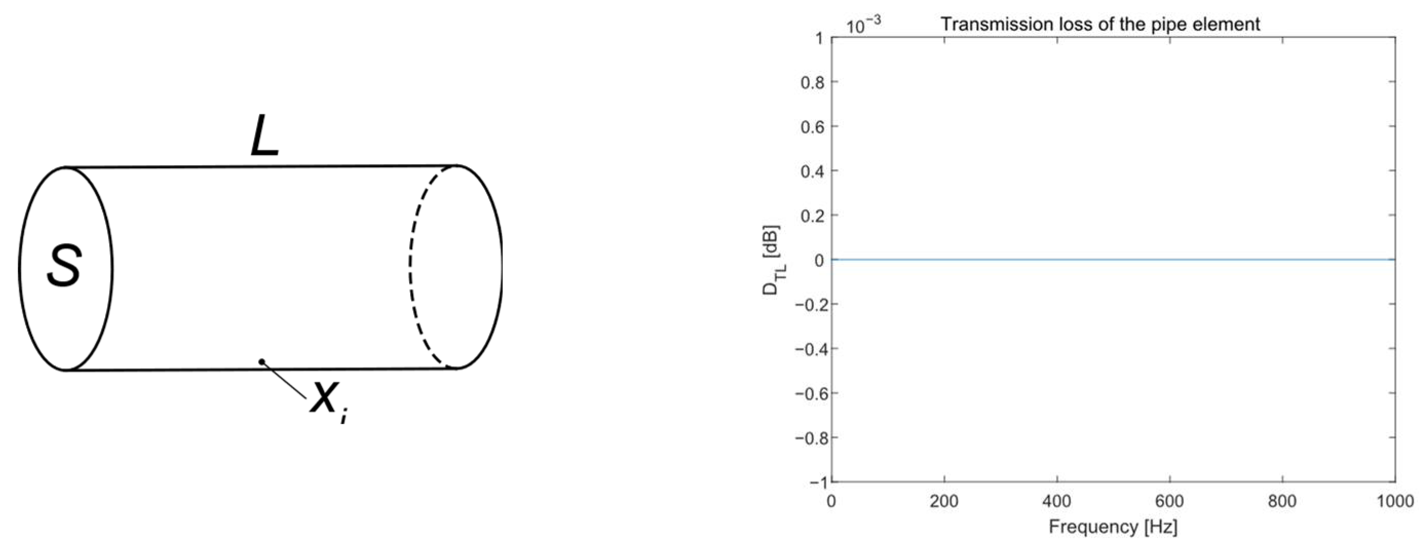
Straight pipe elements are found in all duct systems, and they usually add only a very small dissipation per meter length to the noise propagating in the duct. The T-matrix for a straight pipe, length L (Figure 3), is:
where K = ω/c is the wave number, c is the speed of sound in air, ω is the angular frequency, ⍴ is the air density, S is the pipe cross section area, and Z = ρc is the acoustic impedance of the air inside the duct.
3.2.2. Expansion Chamber
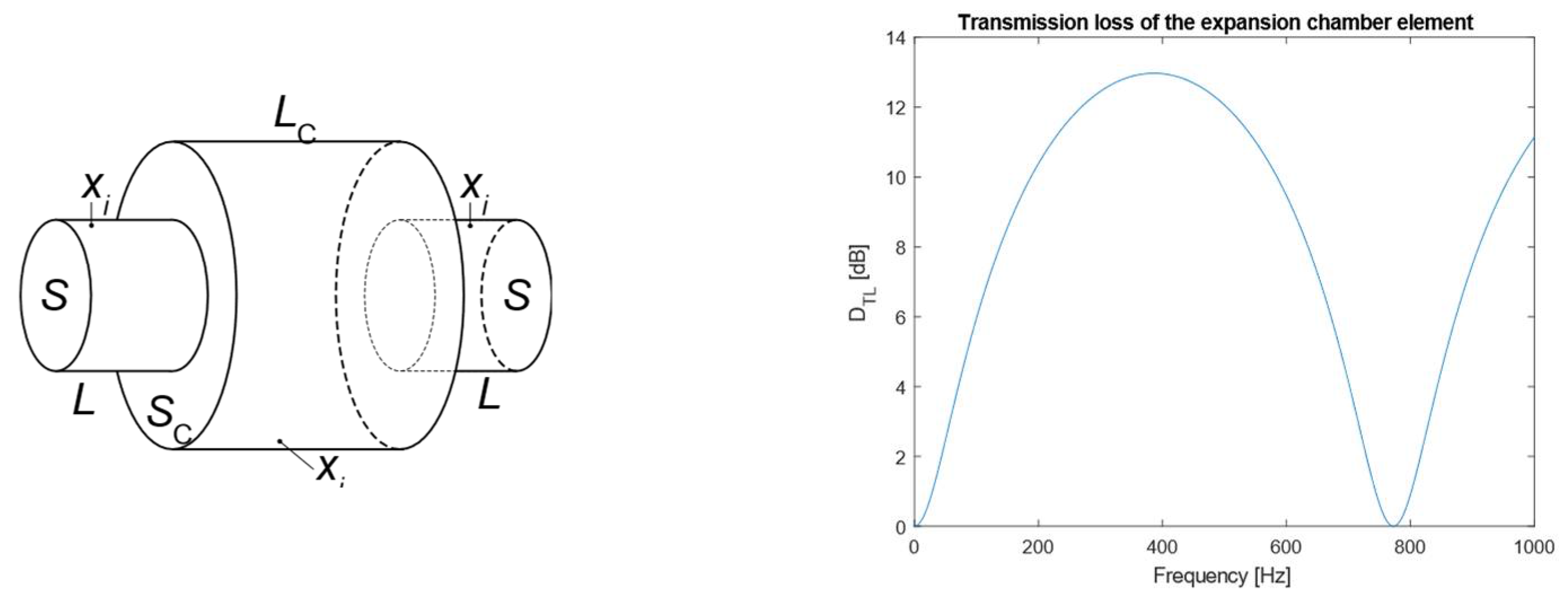
This element features an area expansion followed by an area contraction, resulting in a double reflection. The attenuation depends on the inlet/outlet cross section areas, main chamber cross section area, and the length of the expansion chamber. An expansion chamber can be considered as being made up of three straight pipes, where the middle pipe has a larger cross section area (Figure 4). Its T-matrix is:
where T2 is the intermediate pipe T-matrix.
When using an expansion chamber, the maximum TL is found by:
where c is the speed of sound and L is the length of the expansion chamber. This device has a broadband attenuation, which is positive in the case of wideband noise. On the other hand, the attenuation is not extremely high, so if a large attenuation is required at specific frequencies, it is suggested to use other types of reactive devices such as a quarter-wavelength resonator or a Helmholtz resonator.
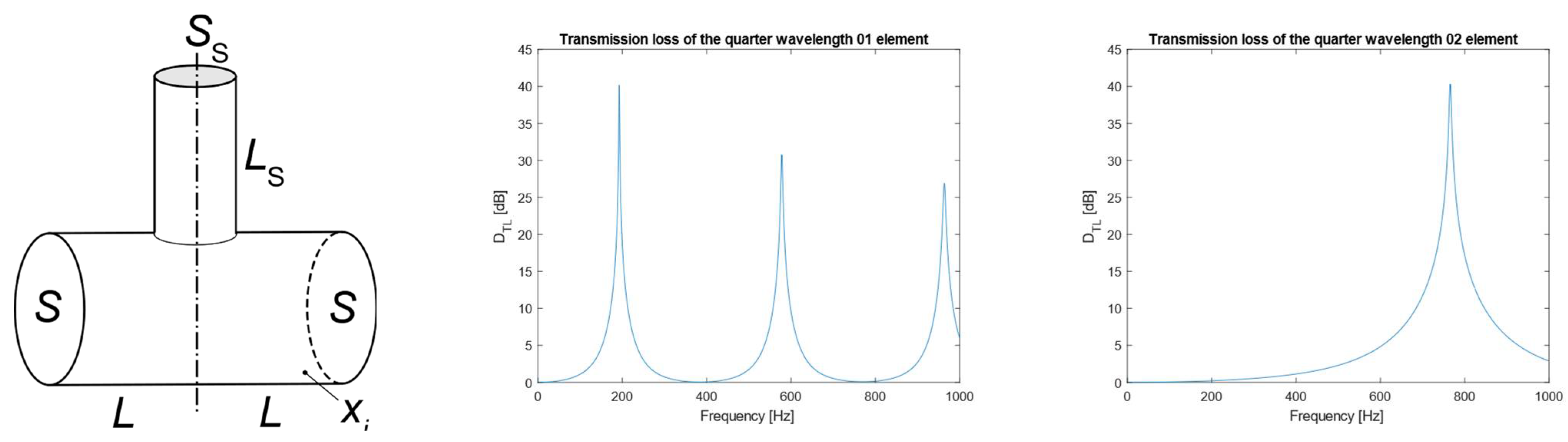
3.2.3. Quarter-Wavelength Resonator
Quarter-wavelength resonators behave like expansion chambers in that they are based on multiple reflections but are characterized by a more selective behavior given by the finite size of the side cavity. A quarter-wavelength resonator is a type of side-branch. In the plane wave frequency region, a side-branch T-matrix can be written as:
where Ss is the side-branch inlet cross section area and Zs is its specific acoustic input impedance seen from its inlet. The specific acoustic input impedance for the quarter-wavelength resonator is:
where Ls is the resonator length. Losses in the resonator are accounted for by the medium complex adiabatic compression modulus, β = β∙(1 + iη), where η is the medium internal loss factor. For this reason, the speed of sound, c = c∙(1 + iη/2), and the wave number, K = ω/c, turn out to be complex-valued.
Equation (12) is the T-matrix for the side-branch seen from its coupling surface with the main duct. For the real physical side-branch, there are also inlet and outlet pipes, both with length, L; see Figure 5. Consequently, the physical quarter-wavelength resonator T-matrix corresponds to the matrix product:
where T1 and T3 are the T-matrices of the straight pipes with length, L, and cross section area S. T2 is the side-branch T-matrix, Equation (12), with side-branch input impedance, Zs, expressed according to Equation (13).
This component provides a high TL at some specific frequencies. The maximum TL is obtained for:
with
thus
Equation (15) shows that the quarter-wavelength resonator size can be significant. For example, for tuning the element at a frequency of 100 Hz, the quarter-wavelength resonator side branch length must have a characteristic length of 0.85 m. It is worth noting that a quarter-wavelength resonator with such a length sometimes cannot be easily fitted in a real system. A common solution for this issue is to bend the resonator or fold it along the main duct axis so that it occupies a space compatible with the overall duct dimension while maintaining its characteristic length.
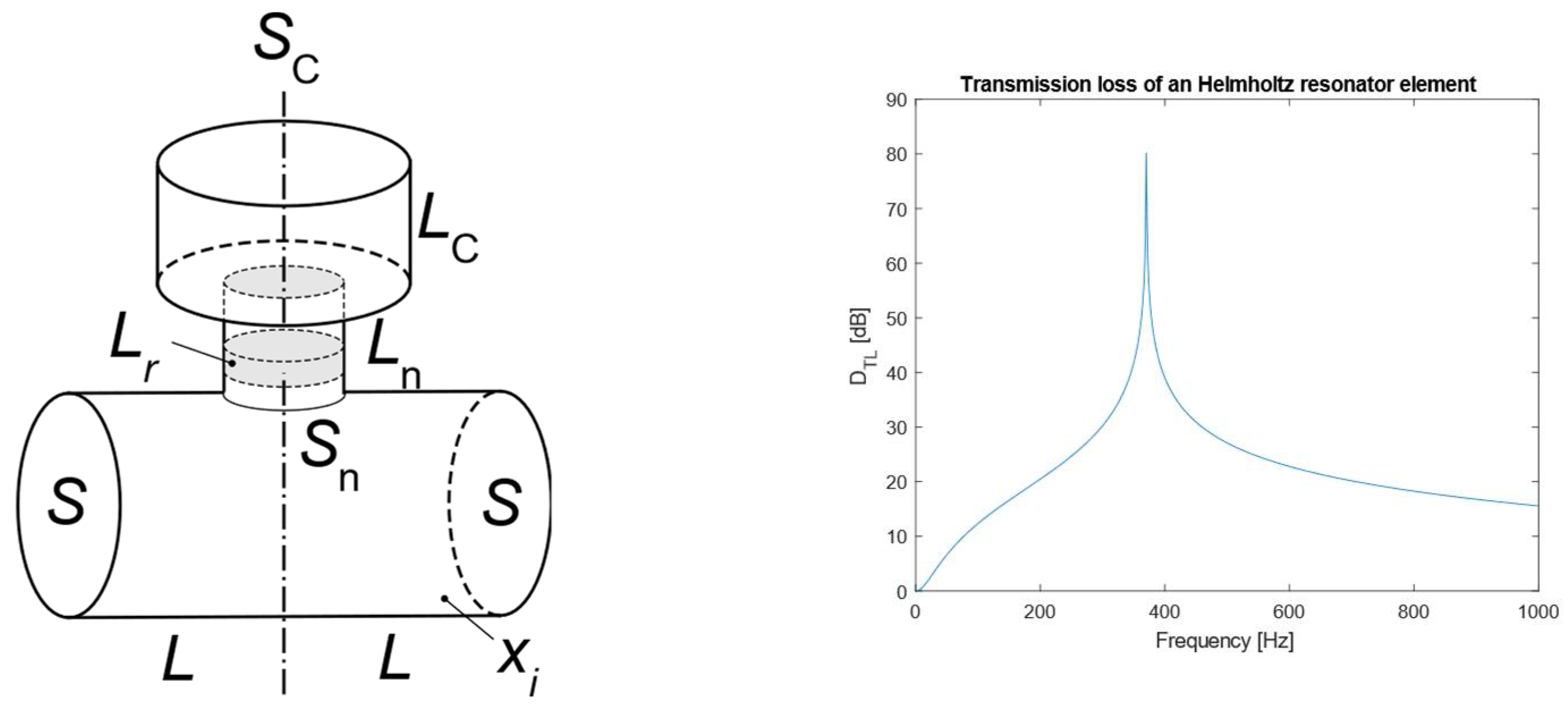
3.2.4. Helmholtz Resonator
The Helmholtz resonator (Figure 6) is a side-branch with a specific input impedance:
where Vc is the resonator volume given by Lc and Sc (see Figure 6). Resonator losses are often generated by a damping material placed in the resonator neck. Such a term is accounted for by introducing the resistance, R. The resistance is determined by the resistivity r [Pa·s/m2] and the damping material length, Lr:
The T-matrix is calculated with (12), where the side-branch acoustic inlet impedance, Zs, is obtained from Equations (18) and (19).
The Helmholtz resonator can be considered as a mass-spring system where an additional inductance (mass of air in the neck of the resonator) is placed between the main duct and the cavity (compliance of the air in the resonator volume acting as a spring). The Helmholtz resonator is highly selective and provides an important attenuation for one specific frequency that depends on the size of the main duct and on the geometry of the resonator. The Helmholtz resonance frequency, not considering the damping material, can be computed as:
It is worth noting that, due to the very low value reached by the side branch impedance at the resonance frequency, the particle velocity at the neck of the resonator can be extremely high. For this reason, a sort of “blockage” appears at the inlet of this component, requiring a “length correction”. In this case, for a circular pipe with a diameter, D, the neck length, Ln, can be modified according to [36]:
- Circular pipe in baffle: ΔL = 0.82 D/2;
- Free end circular pipe ΔL = 0.61 D/2.
A last comment concerns the effect of increasing the inner losses of a Helmholtz Resonator (as well as of a quarter-wavelength resonator). When a material expressing a certain flow resistivity is placed in a side branch, the effect is to slightly reduce the maximum of the attenuation at the resonance frequency/ies, increasing at the same time the frequency width of the peak. This behavior can be used to make the attenuation capability of the element less sharp, and then to make it more flexible in the reduction of noise in the frequency range around the resonance peak. To take into account such behavior, the software can compute the effect of an absorbent layer with a flow resistivity, r, and a thickness, Lr, placed over the neck cross section.
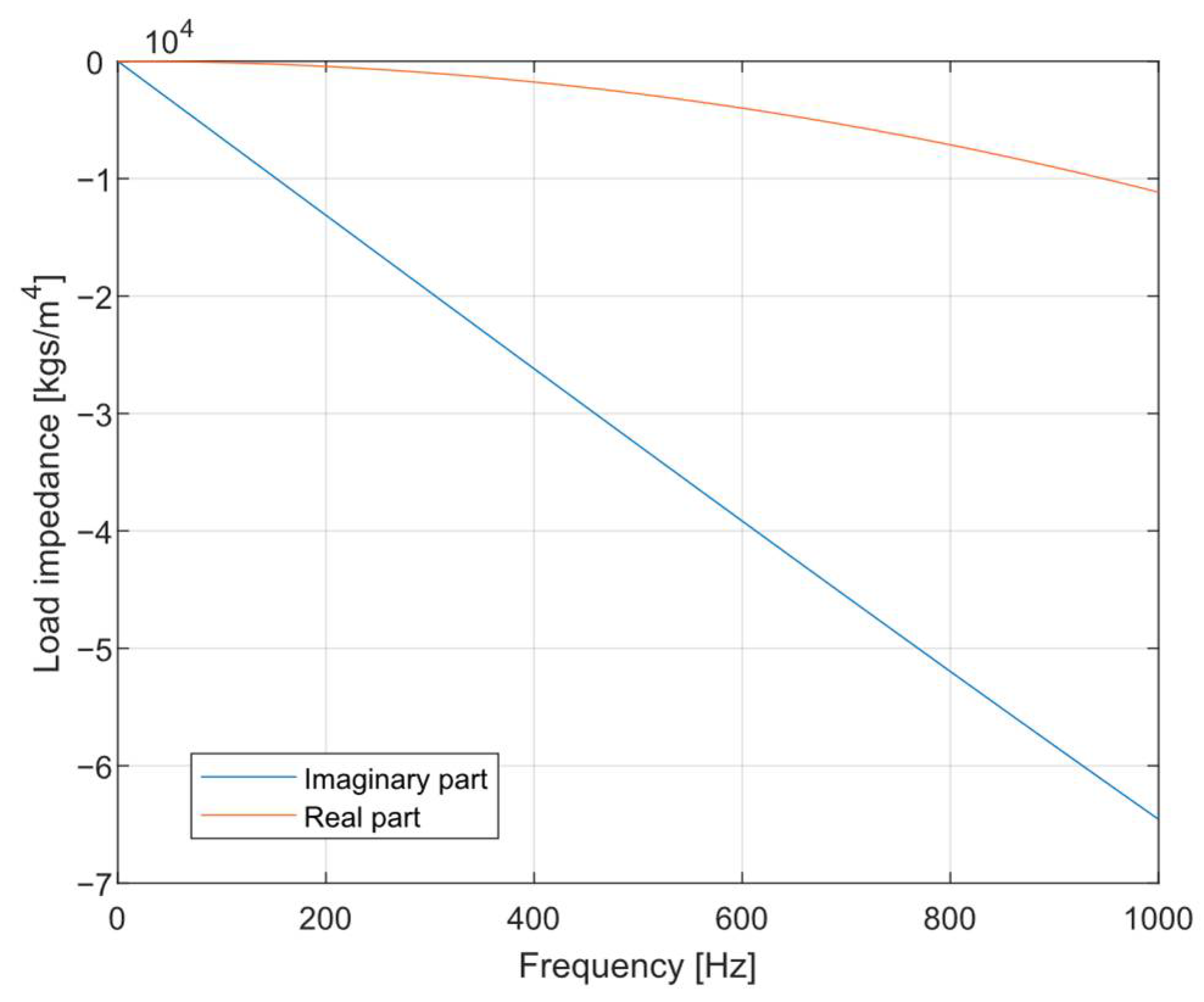
3.3. Outlet Impedance Model
To account for the outlet impedance, a formulation for the radiation impedance, Zr, by Silva et al. for the un-flanged case is used [39]:
where a is the duct radius, k is the wavenumber, and the coefficients d1 = 1.393, d2 = 0.457, and n1 = 0.167 are the result of a numerical fitting. The radiation impedance, Zr, is then multiplied by ρ0c/Sout to obtain the outlet impedance, ZL. Figure 7 shows the real and imaginary parts of the outlet impedance as a function of frequency for a duct of diameter 45.2 mm.
3.4. Pressure Drop Estimation
Aerodynamic losses cause a pressure drop when the air flows through a duct. This energy loss reduces the flow speed and the system efficiency. Therefore, it should be made as small as possible. A good duct and silencer design has a high noise reduction and a low pressure drop. Because the pressure drop is caused by the mean flow, we assume that the pressure drop caused by side-branches with zero mean flow is negligible. In the expansion chamber we have a mean flow and, hence, a possibly significant pressure drop. Below a simple pressure drop estimation method, Darcy’s friction factor method is described.
The method divides the pressure drop in two generation mechanisms. The first is the contribution from the friction force between the flowing medium and the duct wall. The second is the contribution from the flow separation appearing at discontinuities such as a sudden cross section area increase. The pressure drop caused by friction between the flowing medium and the duct wall is estimated with:
where X is Darcy’s friction factor, U is the mean flow speed, L is the pipe length, and D is the pipe hydraulic (wet) diameter. Normally, the hydraulic diameter is equal to the pipe inner diameter. At a sudden cross section area increase, we estimate the flow separation pressure drop with:
where the “friction” factor Xs is
where S1 and S2 are the cross-sectional area at the inlet and at the outlet of the sudden cross-section increase or decrease, respectively. The pressure drop caused by a sudden cross section area decrease is assumed to be negligible. U1 in Equation (23) is the mean flow speed at the inlet where the cross-section area is S1. The total pressure drop over the n-th element is the sum of its friction and flow separation losses:
Finally, the total pressure drop over the duct system is the sum of the contributions from all N elements:
This quantity can be useful when sizing the ventilation system. Because this work focuses on the acoustic aspects of the design procedure, pressure drop results will not be presented in the following.
4. Materials and Methods
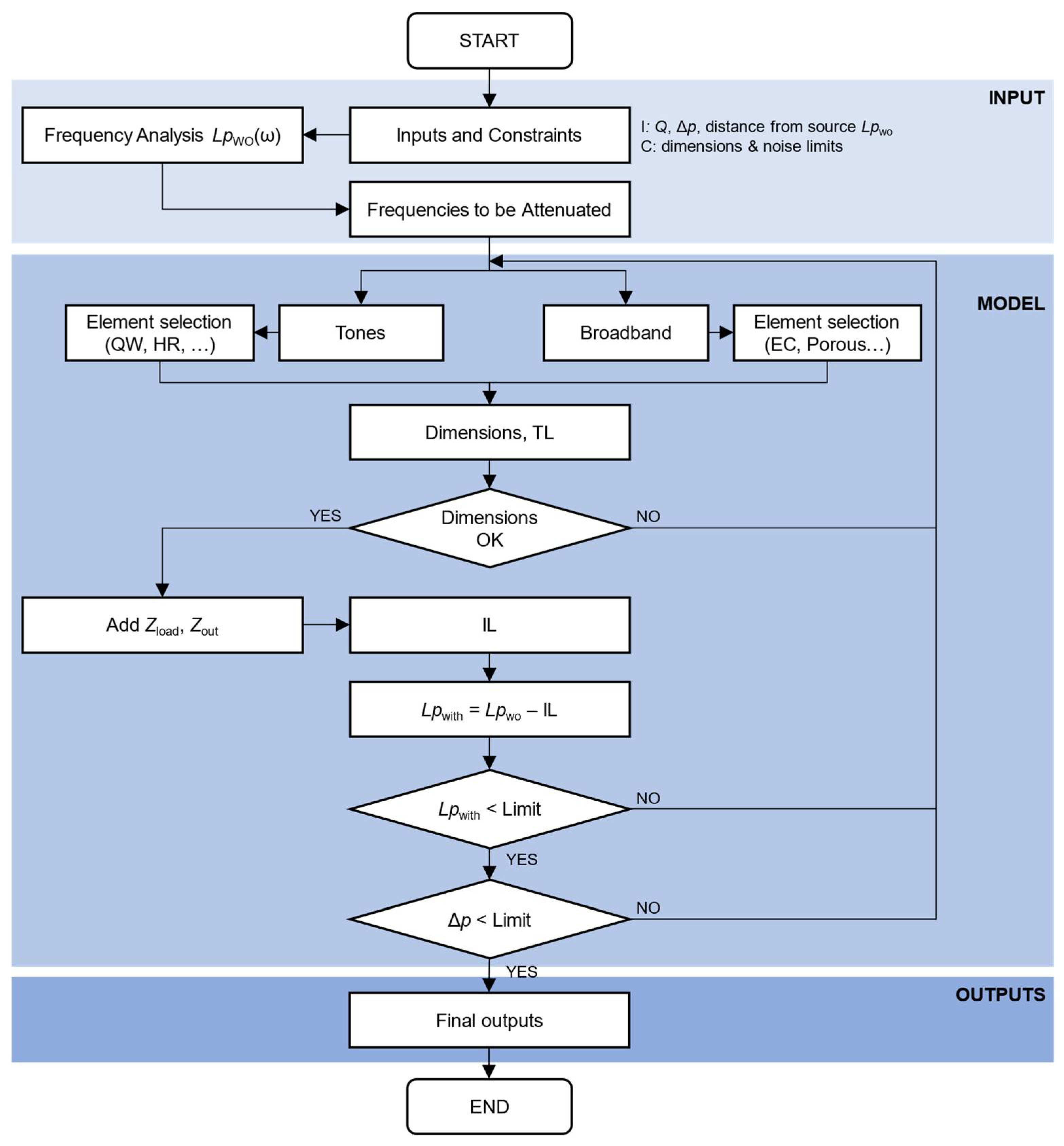
4.1. Outline of the Complete Design Procedure
The TMM theory reported in Section 3 is the core of the design procedure outlined in Figure 8, which can be roughly summarized in the following steps:
- Definition of objectives and design constraints;
- Identification of the frequency components to attenuate;
- Selection of reactive elements and of their sequence;
- Application of TMM method;
- Verification of objective achievement in terms of SPL;
- Verification of design constraint respect;
- Definition of the final solution.
Steps 1–2 form the inputs to be passed to the xTMM method. Step 2 consists of looking at the one-third octave spectrum and identifying the one-third octave bands where noise reduction is required. Then, a second check on the narrow band sound pressure level spectrum allows one to identify the narrow band frequencies where noise reduction measures are needed. The narrow band frequencies are the ones to be used for dimensioning the silencer elements.
Steps 3–6 are carried out through a manual iterative process: in particular, if design criteria, such as size limits, or SPL objective are not fulfilled with the current trial solution, a new element combination must be devised, and steps 3–6 must be repeated. This manual iterative block can be replaced by an optimization algorithm to automatically provide the best element sequence, which is beyond the scope of this work, without modifying the procedure framework.
Step 3 is carried out by investigating the transmission loss for the available silencer elements (quarter-wavelength resonator, Helmholtz resonator, and expansion chamber). In this way, it is possible to make an estimate on which elements to apply, especially when it is necessary to have a high transmission loss at more than a single frequency. In this case, it is interesting to note that while a quarter-wavelength resonator expresses a high TL at odd “resonance frequencies” with a high selectivity (sharp peaks), an expansion chamber has a less sharp TL characteristic (see Figure 4 and Figure 5, respectively). This behavior allows one to have a good TL over a wider frequency range. The position of the frequencies with the higher TL is usually determined by the length of the element, while the amount of reduction for an expansion chamber is controlled by the diameter of the expansion chamber. The real silencer system is built up using silencer elements and straight coupling pipes. The minimum distance between two silencer elements is set by the dimensions of the coupling elements (T-couplings, area changes, and muffs).
When all silencer elements are created, they can be combined to build the silencer system, and it is possible to calculate the overall properties: the length, the TL, and the IL (step 4 in the procedure outlined above). The elements must follow a sequence for the correct implementation of the T-matrix product, with the first element representing the element closest to the source, and so on. The total TL is calculated, and the first check on the dimensions is performed (step 5). As discussed in Section 3, the IL depends on the source and receiver impedances, thus the loudspeaker impedance must be determined. When the IL has been calculated, the system contribution to the sound in the observation point can be computed and compared with the requirement. The fulfillment of the SPL objective is checked at this stage (step 6) and, if necessary, adjustments to the solution are made, from a simple rearrangement of the elements to the complete re-design of the system, until all the requirements are satisfied. Depending on the specific situation, pressure drops can also be part of the acceptability criteria.
The solution provided in step 7 is a silencer that satisfies the noise attenuation objective while respecting all the system design constraints.
4.2. Validation of the Silencing System
Once a system satisfying all the requirements has been modeled, a prototype can be built for experimental validation. A simple sketch showing all the relevant information can be prepared at this stage, taking care of specifying all the necessary internal dimensions. The construction part must follow a certain path:
- Cut the pipe elements and assemble the silencer system according to the sketch;
- Measure the background noise;
- Mount the silencer system in a test rig and measure the SPL frequency spectrum in the observation point at a desired distance from the outlet;
- Measure the reference system SPL in the observation point;
- Calculate the silencer system insertion loss from the measured data.
It is important to build the silencer system such that it agrees with the silencer design stage. An accurately built silencer system has a good chance to show good agreement with the theoretical results in the experimental validation. For this reason, the following specifications must be carefully checked for compliance with the design sketch:
- Center-to-center distances between side branches (quarter-wavelength resonators, and Helmholtz resonators);
- Internal expansion chamber lengths;
- Distances from components, side branch centers, expansion chamber inner walls, etc., to duct inlet/outlet.
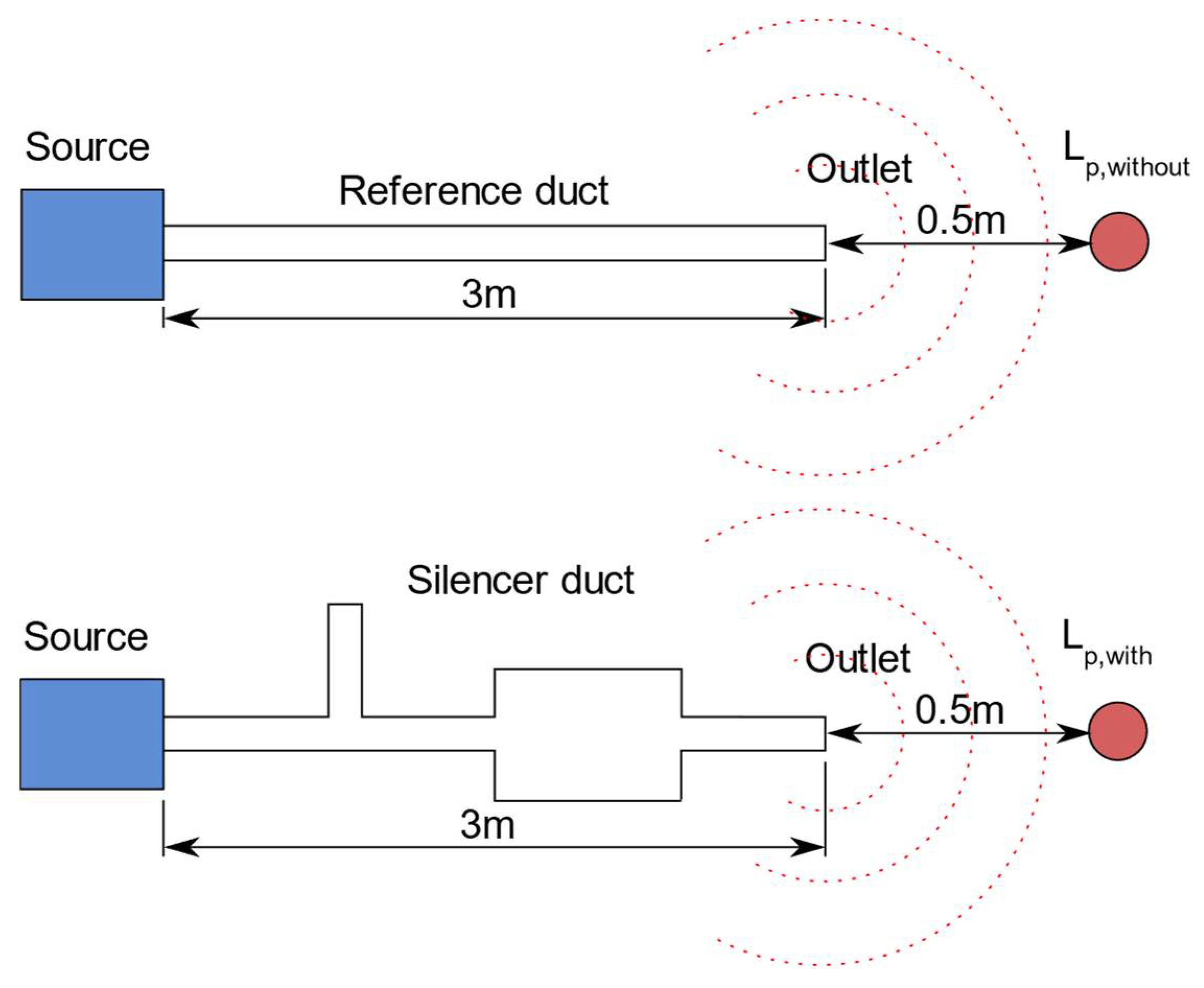
According to the definition, the silencer IL can be estimated as the difference of the SPL between the system with a reference duct (Lp,without) and the system with the silencer (Lp,with):
In the validation measurement, the observation point is placed on the duct axis. For example, in Figure 9 the observation point is placed 0.5 m from the outlet. The source used in the measurement must be the loudspeaker used in the simulations.
The procedure to follow to calculate measurement-based IL is:
- Attach the reference pipe to the loudspeaker;
- Place the microphone in the observation point on the duct axis at the desired distance from the outlet;
- Measure the sound pressure, pwithout, using pink or white noise excitation signal;
- Replace the reference pipe with the silencer duct;
- Measure the sound pressure, pwith, using the same signal;
- Switch off the source;
- Measure the background sound pressure, pbackground;
- Remove the contribution of the background noise from the measured RMS sound pressures for both the measurements;
- ;
- Calculate the reference duct and silencer duct sound pressure levels;
- Calculate the IL.
5. Case Study
5.1. Objectives and Application of xTMM Design Procedure
The validation of the procedure has been carried out at the University of Brescia as part of an advanced course addressed to students and practitioners in the field of acoustics and vibration. To verify the capability of the method and the usability of the calculation tool, four groups of participants were asked to carry out the complete procedure to design a silencer, including selection of components and experimental validation of the system. The steps to follow involve designing, building, and experimentally validating a silencer setup mimicking a small ventilation system located in a building. The objective was to reduce the sound pressure level at 0.5 m from the outlet of a pipe arrangement representing a ventilation system. In detail, the A-weighted Sound Pressure Level (SPL) at an observation point placed at 0.5 m from the outlet on the duct axis must not exceed 55 dB(A). The reason for imposing such a limit is that, during a normal conversation, the A-weighted SPL measured at 1 m distance from the speaker is approximately 65 dB(A). By requiring the ventilation system contribution to be lower than 55 dB(A), a reasonably good sound environment for a conversation is achieved [49].
As the starting point, a real or simulated ventilation system sound and a calibration file for scaling the sound data were made available. These files can be used to characterize the basic ventilation system, consisting a straight pipe, 3 m long, with an inner diameter of 45.2 mm. The ventilation system has only one outlet. For practical implementation reasons, it is assumed that the silencer components can be placed anywhere from 0.5 m from the inlet to 0.3 m from the outlet. Any cascade combination of silencer element types is allowed. The silencer elements are connected through straight pipes, 45.2 mm diameter, meaning that the cut-on frequency of the main duct is 2200 Hz. The chosen silencer elements are mounted in series. In the practical implementation, for comparison reasons, the total length of the duct, including the silencing elements, must be exactly 3 m (from inlet to outlet, see Lsystem in Figure 10).
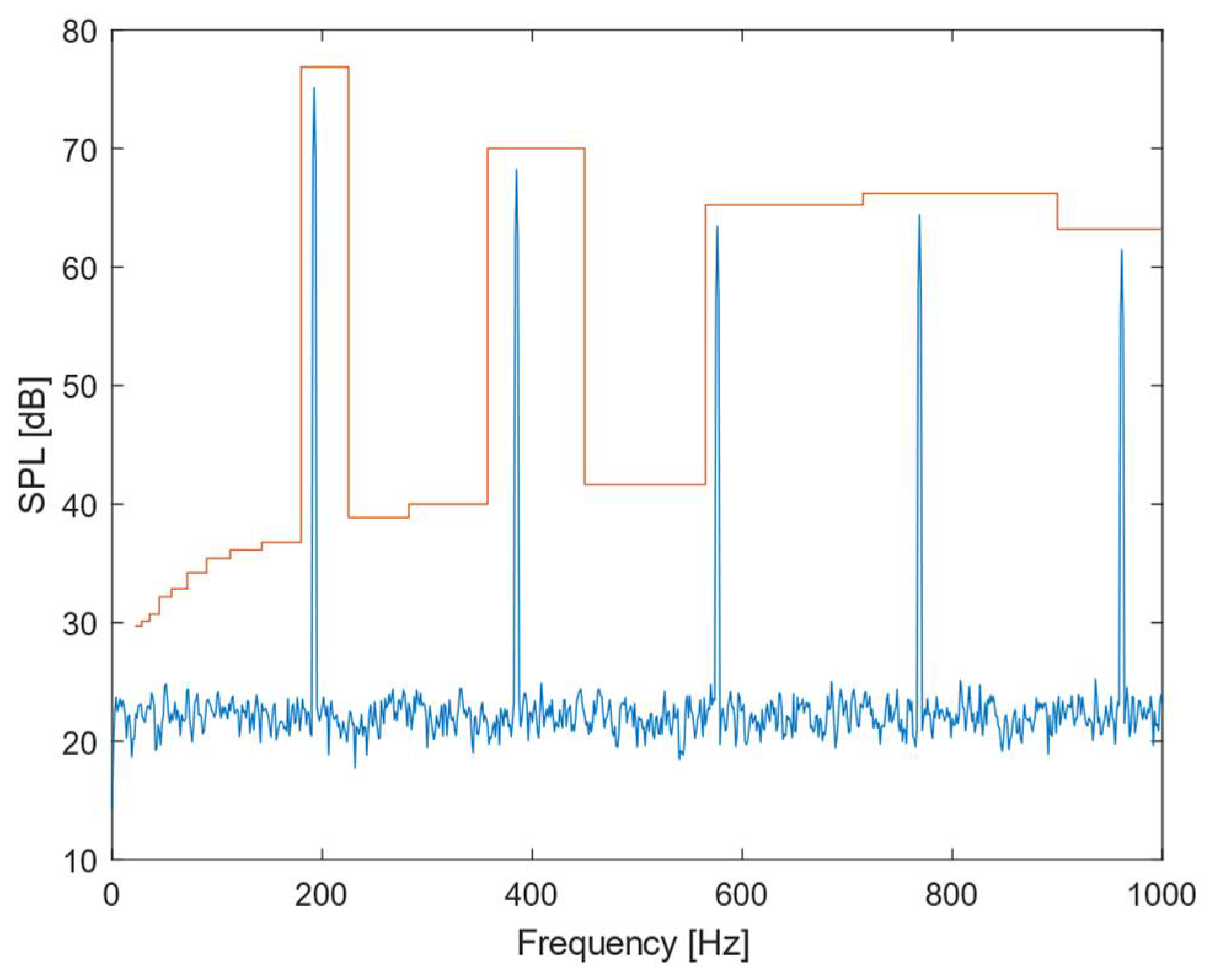
Before selecting the components able to properly attenuate the SPL at the outlet and design a suitable silencer system, the SPL frequency spectrum at the observation point was determined as a signal representing a measurement of the noise generated by a ventilator, together with a certain quote of broad band noise. The SPL was derived by post processing the waveform Audio File Format, simulating the signal recorded by a microphone at the reference position at 0.5 m from the duct outlet. The post processing was carried out by performing an FFT analysis of the signal and computing the one-third octave band spectrum. The latter information is extremely useful because it allows one to determine which frequencies give the highest contribution. Based on the narrow band spectrum, it is possible to make a first estimation of the dimensions of the reactive components by using Equations (11), (17), and (20). The signal needs to be properly averaged to obtain a clear idea about the amplitude of the reductions. For this reason, a synthesis of the FFT spectrum to one-third octave band analysis allows an estimation of the broad band noise and of the A-weighted sound pressure level at the observation point. In the case at hand, the noise at the receiver position for a 3 m long straight pipe is shown in Figure 11. It is worth observing that the noise presents some well-defined components at 192.5 Hz, 385 Hz, 576 Hz, 768 Hz, and 961 Hz. These are the frequencies to be targeted by the implementation of specific reactive elements.
The one-third octave bands where the A-weighted SPL exceeds the maximum allowed level of 55 dB(A) were then decremented by a “first trial” insertion loss of 20 dB (see Table 1). The 20 dB value is merely an indicator that points out for which bands it is necessary to reduce the noise, and it does not specify the amount of reduction required by the individual silencer components. Once the 20-dB IL is applied to the selected bands, the resulting overall sound pressure level was successfully checked to verify that it was below the objective value of 55 dB(A). Had not this been the case, additional IL should also have been applied for the highest remaining one-third octave bands. The required A-weighted SPL at the receiver, LA,req, was then calculated as:
The results of the calculations are reported in Table 1. It can be observed that in this example it is necessary to apply a reduction at the 200 Hz, 400 Hz, 630 Hz, 800 Hz, and 1000 Hz 1/3 octave bands.
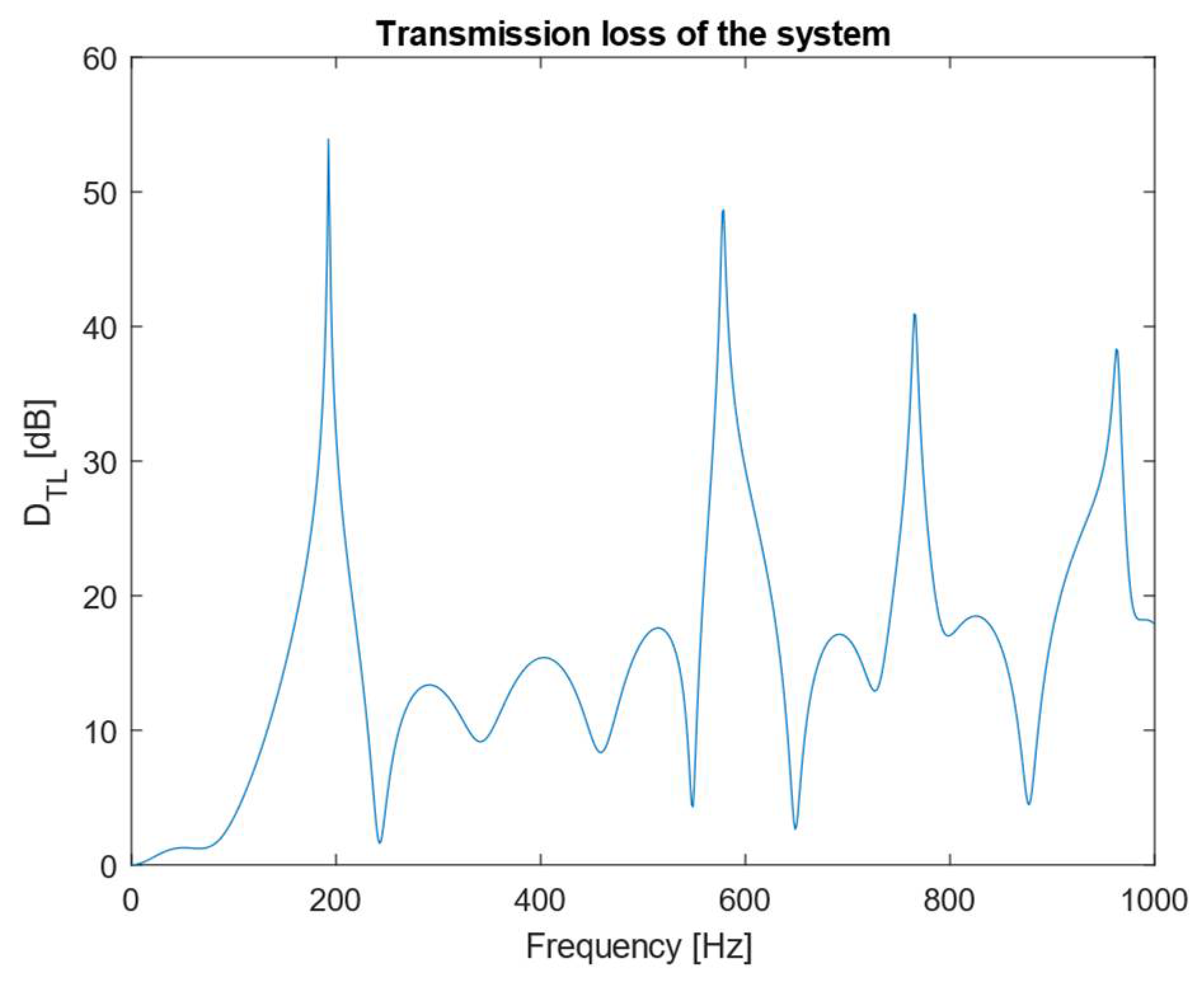
The estimation of the dimensions of the elements required to properly attenuate the targeted frequency components was therefore carried out by recalling the shape and the frequency values of the different elements, and by proceeding with heuristic reasoning. For example, the first group of participants started from a 192.5 Hz component, where a good attenuation can be obtained with a quarter-wavelength resonator. The length of a resonator tuned at this frequency, assuming a speed of sound equal to 343 m/s, is 0.445 m. Such elements can also be used to attenuate other frequencies and can be obtained by multiplying the fundamental frequency by odd natural numbers (for n = 3, f3 = 577.5 Hz, for n = 5, f5 = 962.5 Hz). This means that, with a single quarter-wavelength resonator, it is possible to cover three-out-of-five noise components. The other component at 385 Hz can be removed by using a 0.222 m expansion chamber, whereas the peak at 768 Hz is attenuated with a second, smaller quarter-wavelength resonator. To summarize, the final implementation of the system devised by the first group is made by using a 0.222 m long expansion chamber for eliminating the 385 Hz peak, a 0.112 m long quarter-wavelength resonator to attenuate the 768 Hz component, and a 0.445 m quarter-wavelength resonator to attenuate the other three frequencies of interest. For the sake of completeness, the TLs of the individual elements used in this solution coincide with the graphs in Figure 4 and Figure 5, whereas the TL of the complete system is shown in Figure 12.
5.2. Results and Discussion
In this section, the outcome of the design procedure applied to the case study described in the previous Section is presented, together with an experimental validation. In particular, the results refer to the solution devised by the first group, including two PhD students in acoustics and vibration subjects, and a third-year Mechanical Engineering student. The drawing showing the practical application of the proposed solution scheme is represented in Figure 13.
As concerns the cross-section dimension of the expansion chamber, it was chosen to be equal to 134 mm for practical reasons related to the availability from the local shops of pipes for the implementation of the test rig. The following step was to build the actual system by cutting pipes with the same length of the components used during the design stage. After preparing the 3 m long straight pipe (reference pipe), all the parts represented in Figure 13 were cut. The real silencer system was developed in collaboration with the Technical and Industrial Design Laboratory of the University of Brescia, which develops devices for research and teaching purpose based on the “study—model” approach typical of industrial design product development [50].
Being cheap, effective, quick to build, and based on commercial parts were key requirements for this application. The arrangement was therefore conceived as a modular system based on push-fit PVC wastewater pipes. The straight parts were the only customized pieces and were cut to well-defined sizes. For the construction of the expansion chambers, a range of pipes with different diameters and lengths was provided. The end of the cylinder and the piston body were made of plywood, and an O-ring was placed in a recess of the piston to ensure airtightness. The inlet and the outlet pipes were made using 50 mm external diameter pipe terminations, as illustrated in Figure 14. Quarter-wavelength resonators were made using a T-branch and a vertical pipe. Plywood pistons with an O-ring seal and a rod fitted with a handle for adjusting the position of the sliding piston were integrated in the design of the components.
Figure 15 shows the system assembled before the tests. To avoid flanking transmissions, the source was enclosed in a wooden box filled with absorbing material. The pipes and the other components were suspended using wooden legs. On the top parts of the pipes used to build the quarter-wavelength resonators, the handles for moving the pistons are clearly visible.
To measure the SPL at 0.5 m from the outlet, an OROS Type OR36 analyzer was connected to a Bruel & Kjaer Type 4189 microphone. The measurement chain was calibrated using a Bruel & Kjaer pistonphone Type 4228. The loudspeaker was fed with a broadband white noise ranging from 50 Hz to 5000 Hz.
A series of measurements were made in the reference situation (3 m long straight pipe) and on the complete system to evaluate IL. In detail, the background noise, the noise coming from the outlet using the straight pipe, and the noise coming from the outlet when the silencer system is installed were evaluated at the receiver position. The results of these measurements are shown in Figure 16. It is worth noting that, because the pink noise is generated starting from 50 Hz, below such frequency there is only a slight difference between the three measurements.
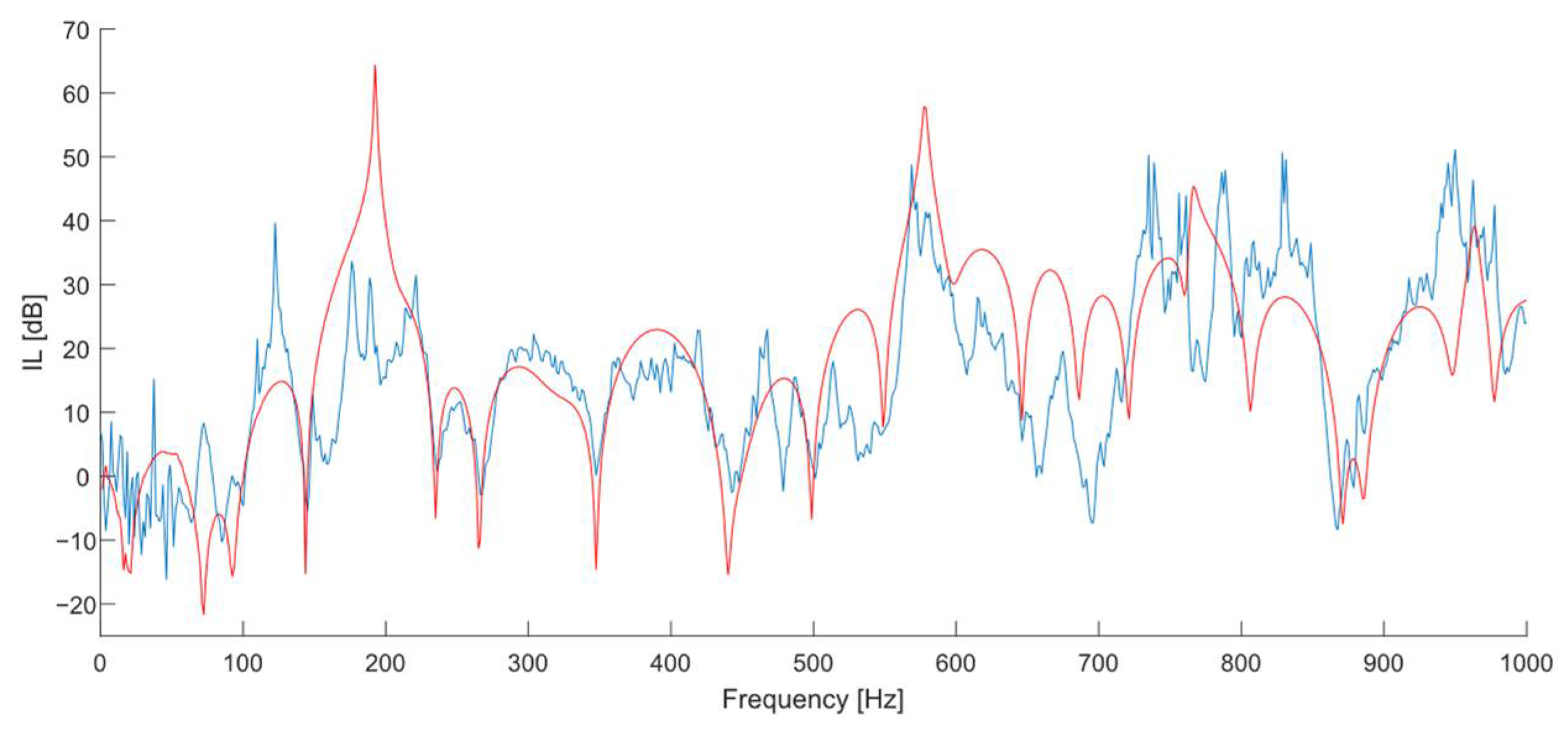
The measured SPLs without and with the silencer system were corrected to consider the background noise, thus it was possible to compute the IL. Figure 17 shows a comparison between measured and predicted curves. Below 50 Hz, the effect of the silencer system can hardly be spotted, but above this frequency the prediction follows quite well the experimental data. The discrepancy around 700 Hz and 750 Hz between the predicted and the measured IL may be due to the noise radiated by the low-density commercial pipes used for the experiments (0.27 kg/m). For the same reason, as can be seen in Figure 15, there are some frequency components in the measured SPL for the complete system (which is longer than the basic one) that are higher than the ones measured for the 3 m long straight pipe.
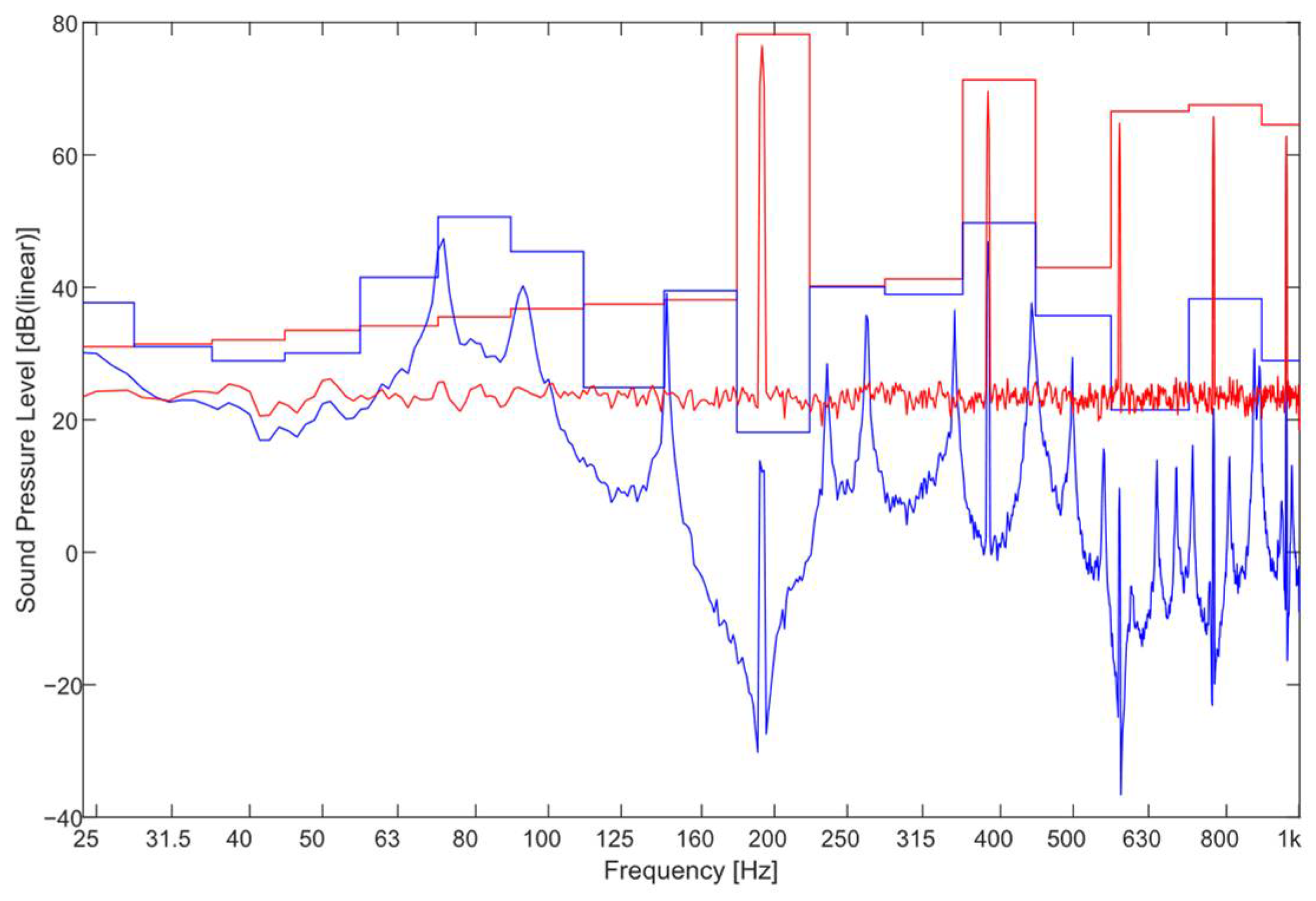
Applying the obtained IL, the resulting A-weighted SPL at the receiver is equal to 51.2 dB(A), and thus the requirement of SPL < 55 dB(A) is fulfilled. In Figure 18, the predicted SPL spectrum at the receiver is plotted in narrow band and in one-third octave bands.
As a final remark, it is worth noting that all four groups involved in the project managed to successfully design their silencing system by proposing different solutions. All participants provided positive feedback on the intuitiveness of the procedure and on the usability of the tool, showing that the method can be efficiently applied in real contexts.
6. Conclusions
The noise coming from ventilation systems can be an annoying issue for applications requiring high quality standards. While it is usually relatively simple to find a solution for the noise propagating above the cut-on frequency, below this limit it is necessary to use reactive components that can be represented through an electro-acoustic analogy. However, the evaluation is generally carried out in terms of sound transmission loss of the system, which is not immediately relatable to human perception.
This article has shown how the classic transfer matrix method theory for the prediction of a reactive silencer’s transmission loss can be expanded to allow the direct evaluation of sound pressure level at a given distance from the outlet. A self-developed tool with possible academic and professional application has been used to demonstrate the potentiality of the method and validate it against experimental results by four groups of students and practitioners attending an advanced course in acoustics and vibration. The outcomes of this study are two-fold: on the one hand, the method, though relying upon relatively simple models of components and acoustic loss factors, provided noise reduction results close to the experimental evidence; on the other hand, the implementation of this expanded framework into a user-friendly tool proved to be an effective way to foster noise-oriented solutions and contribute to creating comfortable environments. Possible future developments include the implementation of optimization strategies to automatize the choice of the components, their characteristic dimensions, and their sequence in order to obtain the desired noise reduction performances with given design constraints.
Author Contributions
Conceptualization, U.E.C. and S.B.; methodology, U.E.C. and S.B.; software, U.E.C., E.A.P. and S.B.; validation, E.A.P. and U.E.C.; formal analysis, S.B.; investigation, E.A.P. and D.P.; resources, E.A.P., A.M.L. and D.P.; data curation, E.A.P. and U.E.C.; writing—original draft preparation, E.A.P.; writing—review and editing, U.E.C. and A.M.L.; visualization, D.P. and E.A.P.; supervision, A.M.L. and S.B. All authors have read and agreed to the published version of the manuscript.
Funding
This research received no external funding.
Institutional Review Board Statement
Not applicable.
Informed Consent Statement
Not applicable.
Conflicts of Interest
The authors declare no conflict of interest.
References
- Song, H.; Cho, H. Flow Characteristics and Noise Reduction Effects of Air Cleaners of Automobile Intake Systems with Built-in Resonators with Space Efficiency. J. Eng. Res.-Kuwait 2021, 9, 294–302. [Google Scholar] [CrossRef]
- Bae, M.-W.; Ku, Y.J.; Park, H.-S. A study on effects of tuning intake and exhaust systems upon exhaust noises in a driving car of gasoline engine. T. Korean Soc. Mech. Eng. A 2021, 45, 31–40. [Google Scholar] [CrossRef]
- Dahlan, A.A.; Muhamad Said, M.F.; Latiff, Z.; Mohd Perang, M.R.; Abu Bakar, S.A.; Abdul Jalal, R.I. Acoustic Study of an Air Intake System of SI Engine Using 1-Dimensional Approach. Int. J. Automot. Mech. Eng. 2019, 16, 6281–6300. [Google Scholar] [CrossRef]
- Yakar, Ö.; Erol, H. Acoustical System Modelling of the Heavy Truck Air Intake System. Int. J. Heavy Veh. Syst. 2019, 26, 158–174. [Google Scholar] [CrossRef]
- Nadareishvili, G.G.; Galevko, V.V.; Rakhmatov, R.I. Improvement of Acoustic Characteristics of Motor Vehicle Intake System Based on Calculation and Experimental Research. In International Conference on Industrial Engineering; Lecture Notes in Mechanical Engineering Book Series; Springer: Cham, Swizerland, 2019; pp. 2311–2322. [Google Scholar] [CrossRef]
- Vidal, V.; Mann, A.; Verriere, J.; Kim, M.; Ailloud, F.; Henner, M.; Cheriaux, O. Towards a Quiet Vehicle Cabin Through Digitalization of HVAC Systems and Subsystems Aeroacoustics Testing and Design; SAE Technical Paper; SAE International: Pittsburgh, PA, USA, 2019. [Google Scholar] [CrossRef]
- Caniato, M.; Bettarello, F.; Schmid, C.; Fausti, P. The Use of Numerical Models on Service Equipment Noise Prediction in Heavyweight and Lightweight Timber Buildings. Build. Acous. 2019, 26, 35–55. [Google Scholar] [CrossRef]
- Borelli, D.; Gaggero, T.; Rizzuto, E.; Schenone, C. Onboard Ship Noise: Acoustic Comfort in Cabins. Appl. Acoust. 2021, 177, 107912. [Google Scholar] [CrossRef]
- Han, H.; Lee, C.; Lee, K.; Jeon, S.H.; Park, S. Estimation of the Sound in Ship Cabins Considering Low Frequency and Flowing Noise Characteristics of HVAC Duct. Appl. Acoust. 2018, 141, 261–270. [Google Scholar] [CrossRef]
- Borelli, D.; Schenone, C.; Di Paolo, M. Application of a Simplified “Source-Path-Receiver” Model for HVAC Noise to the Preliminary Design of a Ship: A Case Study. In Proceedings of the 21st International Congress on Sound and Vibration 2014, ICSV 2014, Beijing, China, 13–17 July 2014; International Institute of Acoustics and Vibrations: Beijing, China, 2014; Volume 2, pp. 1257–1264. [Google Scholar]
- Altabey, W.A. An Exact Solution for Acoustic Simulation Based Transmission Loss Optimization of Double-Chamber Silencer. Sound. Vib. 2020, 54, 215–224. [Google Scholar] [CrossRef]
- Ray, E.F. Aerodynamics of Ducted Systems and Flow Affects upon Silencers, Combustion Turbines, and Machine Performance. In Proceedings of the 41st International Congress and Exposition on Noise Control Engineering 2012, New York, NY, USA, 19–22 August 2012; INTER-NOISE 2012. Volume 4, pp. 3080–3091. [Google Scholar]
- Yadav, S.; Sharma, G.S. Noise Reduction Techniques for FD & ID Fan in Thermal Power Plant Using Chamber Based Silencer. Int. J. Mech. Prod. Eng. Res. Dev. 2019, 9, 409–420. [Google Scholar] [CrossRef]
- Mimani, A.; Kirby, R. Design of Large Reactive Silencers for Industrial Applications. In Proceedings of the INTER-NOISE 2018—47th International Congress and Exposition on Noise Control Engineering: Impact of Noise Control Engineering, Chicago, IL, USA, 26–29 August 2018; Institute of Noise Control Engineering: Chicago, IL, USA, 2018. [Google Scholar]
- Papini, G.S.; Pinto, R.L.U.F.; Medeiros, E.B.; Coelho, F.B.G. Hybrid Approach to Noise Control of Industrial Exhaust Systems. Appl. Acoust. 2017, 125, 102–112. [Google Scholar] [CrossRef]
- Limacher, P.; Spinder, C.; Banica, M.C.; Feld, H.-J. A Robust Industrial Procedure for Measuring Modal Sound Fields in the Development of Radial Compressor Stages. J. Eng. Gas Turb. Power 2017, 139, 062604. [Google Scholar] [CrossRef]
- Khelladi, S.; Kouidri, S.; Bakir, F.; Rey, R. Predicting Tonal Noise from a High Rotational Speed Centrifugal Fan. J. Sound Vib. 2008, 313, 113–133. [Google Scholar] [CrossRef]
- Velarde-Suárez, S.; Ballesteros-Tajadura, R.; Pablo Hurtado-Cruz, J.; Santolaria-Morros, C. Experimental Determination of the Tonal Noise Sources in a Centrifugal Fan. J. Sound Vib. 2006, 295, 781–796. [Google Scholar] [CrossRef]
- De Laborderie, J.; Moreau, S. Prediction of Tonal Ducted Fan Noise. J. Sound Vib. 2016, 372, 105–132. [Google Scholar] [CrossRef]
- Holewa, A.; Weckmüller, C.; Guérin, S. Impact of Bypass Duct Bifurcations on Fan Noise. J. Propul. Power 2014, 30, 143–152. [Google Scholar] [CrossRef]
- Kabral, R.; Du, L.; Åbom, M.; Knutsson, M. A Compact Silencer for the Control of Compressor Noise. SAE Int. J. Engines 2014, 7, 1572–1578. [Google Scholar] [CrossRef]
- Figurella, N.; Dehner, R.; Selamet, A.; Tallio, K.; Miazgowicz, K.; Wade, R.; Karim, A.; Keller, P.; Shutty, J. Effect of Inlet Guide Vanes on Centrifugal Compressor Acoustics and Performance. Noise Control Eng. J. 2014, 62, 232–237. [Google Scholar] [CrossRef]
- Nagarhalli, P.V.; Maurya, A.; Kalsule Ceng, S.; Titave, U. Optimizing an Automotive HVAC System for Enhancement of Acoustic Comfort. In Proceedings of the SAE Technical Papers; SAE International: Jodhpur, India, 22 September 2021. [Google Scholar]
- Xue, F.; Sun, B. Experimental Study on the Comprehensive Performance of the Application of U-Shaped Corrugated Pipes into Reactive Mufflers. Appl. Acoust. 2018, 141, 362–370. [Google Scholar] [CrossRef]
- Harvie-Clark, J.; Chilton, A.; Conlan, N.; Trew, D. Assessing Noise with Provisions for Ventilation and Overheating in Dwellings. Build. Serv. Eng. Res. Technol. 2019, 40, 263–273. [Google Scholar] [CrossRef]
- Caniato, M.; Schmid, C.; Gasparella, A. A Comprehensive Analysis of Time Influence on Floating Floors: Effects on Acoustic Performance and Occupants’ Comfort. Appl. Acoust. 2020, 166, 107339. [Google Scholar] [CrossRef]
- Bettarello, F.; Fausti, P.; Baccan, V.; Caniato, M. Impact Sound Pressure Level Performances of Basic Beam Floor Structures. Build. Acous. 2010, 17, 305–316. [Google Scholar] [CrossRef]
- Caniato, M.; Marzi, A.; Monteiro da Silva, S.; Gasparella, A. A Review of the Thermal and Acoustic Properties of Materials for Timber Building Construction. J. Build. Eng. 2021, 43, 103066. [Google Scholar] [CrossRef]
- Caniato, M.; Cozzarini, L.; Schmid, C.; Gasparella, A. Acoustic and Thermal Characterization of a Novel Sustainable Material Incorporating Recycled Microplastic Waste. Sustain. Mat. Technol. 2021, 28, e00274. [Google Scholar] [CrossRef]
- Schönfeld, J.C. Analogy of Hydraulic, Mechanical, Acoustic and Electric Systems. Appl. Sci. Res. 1954, 3, 417–450. [Google Scholar] [CrossRef]
- Bodén, H.; Åbom, M. Modelling of Fluid Machines as Sources of Sound in Duct and Pipe Systems. Acta Acust. 1995, 3, 549–560. [Google Scholar]
- Glav, R.; Åbom, M. A General Formalism for Analyzing Acoustic 2-Port Networks. J. Sound Vib. 1997, 202, 739–747. [Google Scholar] [CrossRef]
- Elnady, T.; Åbom, M. SIDLAB: New 1D Sound Propagation Simulation Software for Complex Duct Networks. In Proceedings of the Thirteenth International Congress on Sound and Vibration, Vienna, Austria, 2–6 July 2006; Volume 5, pp. 4262–4269. [Google Scholar]
- Caniato, M. Sound Insulation of Complex Façades: A Complete Study Combining Different Numerical Approaches. Appl. Acoust. 2020, 169, 107484. [Google Scholar] [CrossRef]
- Bilawchuk, S.; Fyfe, K.R. Comparison and Implementation of the Various Numerical Methods Used for Calculating Transmission Loss in Silencer Systems. Appl. Acoust. 2003, 64, 903–916. [Google Scholar] [CrossRef]
- Åbom, M. An Introduction to Flow Acoustics; KTH: Stockholm, Sweden, 2010. [Google Scholar]
- Wallin, H.P.; Carlsson, U.; Åbom, M.; Bodén, H.; Glav, R.; Hildebrand, R. Sound and Vibration; KTH: Stockholm, Sweden, 2014. [Google Scholar]
- Boij, S.; Abom, M.; Pieters, R. Reflection Properties of a Flow Pipe with a Small Angle Diffuser Outlet. In Proceedings of the 17th International Congress on Sound and Vibration 2010, ICSV 2010, Cairo, Egypt, 18–22 July 2010; Volume 1, pp. 706–712. [Google Scholar]
- Silva, F.; Guillemain, P.; Kergomard, J.; Mallaroni, B.; Norris, A.N. Approximation Formulae for the Acoustic Radiation Impedance of a Cylindrical Pipe. J. Sound Vib. 2009, 322, 255–263. [Google Scholar] [CrossRef] [Green Version]
- Elnady, T.; Elsaadany, S.; Herrin, D.W. Investigation of the Acoustic Performance of After Treatment Devices. SAE Int. J. Passeng. Cars Mech. Syst. 2011, 4, 1068–1075. [Google Scholar] [CrossRef]
- Elsahar, W.; Elnady, T. Measurement and Simulation of Two-Inlet Single-Outlet Mufflers. SAE Int. J. Passeng. Cars Mech. Syst. 2015, 8, 1026–1033. [Google Scholar] [CrossRef]
- Piana, E.A.; Uberti, S.; Copeta, A.; Motyl, B.; Baronio, G. An Integrated Acoustic–Mechanical Development Method for off-Road Motorcycle Silencers: From Design to Sound Quality Test. Int. J. Interact. Des. Manuf. 2018, 12, 1139–1153. [Google Scholar] [CrossRef]
- Jiménez, N.; Romero-García, V.; Pagneux, V.; Groby, J.-P. Rainbow-Trapping Absorbers: Broadband, Perfect and Asymmetric Sound Absorption by Subwavelength Panels for Transmission Problems. Sci. Rep. 2017, 7, 13595. [Google Scholar] [CrossRef] [PubMed]
- Long, H.; Cheng, Y.; Liu, X. Asymmetric Absorber with Multiband and Broadband for Low-Frequency Sound. Appl. Phys. Lett. 2017, 111, 143502. [Google Scholar] [CrossRef]
- Boulvert, J.; Humbert, T.; Romero-García, V.; Gabard, G.; Fotsing, E.R.; Ross, A.; Mardjono, J.; Groby, J.-P. Perfect, Broadband, and Sub-Wavelength Absorption with Asymmetric Absorbers: Realization for Duct Acoustics with 3D Printed Porous Resonators. J. Sound Vib. 2022, 523, 116687. [Google Scholar] [CrossRef]
- Long, H.; Shao, C.; Cheng, Y.; Tao, J.; Liu, X. High Absorption Asymmetry Enabled by a Deep-Subwavelength Ventilated Sound Absorber. Appl. Phys. Lett. 2021, 118, 263502. [Google Scholar] [CrossRef]
- Červenka, M.; Bednařík, M.; Groby, J.-P. Optimized Reactive Silencers Composed of Closely-Spaced Elongated Side-Branch Resonators. J. Acoust. Soc. Am. 2019, 145, 2210–2220. [Google Scholar] [CrossRef] [Green Version]
- Stinson, M.R. The Propagation of Plane Sound Waves in Narrow and Wide Circular Tubes, and Generalization to Uniform Tubes of Arbitrary Cross-sectional Shape. J. Acoust. Soc. Am. 1991, 89, 550–558. [Google Scholar] [CrossRef]
- Rusnock, C.F.; Bush, P.M. Case Study: An Evaluation of Restaurant Noise Levels and Contributing Factors. J. Occup. Environ. Hyg. 2012, 9, D108–D113. [Google Scholar] [CrossRef]
- Paderno, D.; Bodini, I.; Villa, V. Proof of Concept as a Multidisciplinary Design-Based Approach. In International Conference of the Italian Association of Design Methods and Tools for Industrial Engineering; Lecture Notes in Mechanical Engineering; Springer: Cham, Swizerland, 2020; pp. 625–636. [Google Scholar] [CrossRef]
Figure 1.
Equivalent acoustic model of a single element—transfer matrix representation.

Figure 2.
A ventilation system with silencer (top) and its linear acoustic system model (bottom). The fan is represented by its acoustic volume flow, QK, and its acoustic impedance, ZK. The silencer system by its T-matrix, T, and the receiving room (load) with its acoustic impedance, ZL.
Figure 2.
A ventilation system with silencer (top) and its linear acoustic system model (bottom). The fan is represented by its acoustic volume flow, QK, and its acoustic impedance, ZK. The silencer system by its T-matrix, T, and the receiving room (load) with its acoustic impedance, ZL.

Figure 3.
Straight pipe sketch (left) and example of TL obtained with TMM (right).

Figure 4.
Expansion chamber sketch (left) and example of TL obtained with TMM (right).

Figure 5.
Quarter-wavelength resonator sketch (left) and examples of TL obtained with TMM (center and right).
Figure 5.
Quarter-wavelength resonator sketch (left) and examples of TL obtained with TMM (center and right).

Figure 6.
Helmholtz resonator sketch (left) and example of TL obtained with TMM (right).

Figure 7.
Real and imaginary parts of outlet impedance of a 45.2 mm diameter tube.

Figure 8.
Flowchart showing the steps to be followed during the design process. QW, HR, and EC indicate quarter-wavelength resonator, Helmholtz resonator, and expansion chamber, respectively.
Figure 8.
Flowchart showing the steps to be followed during the design process. QW, HR, and EC indicate quarter-wavelength resonator, Helmholtz resonator, and expansion chamber, respectively.

Figure 9.
IL measurement outline.

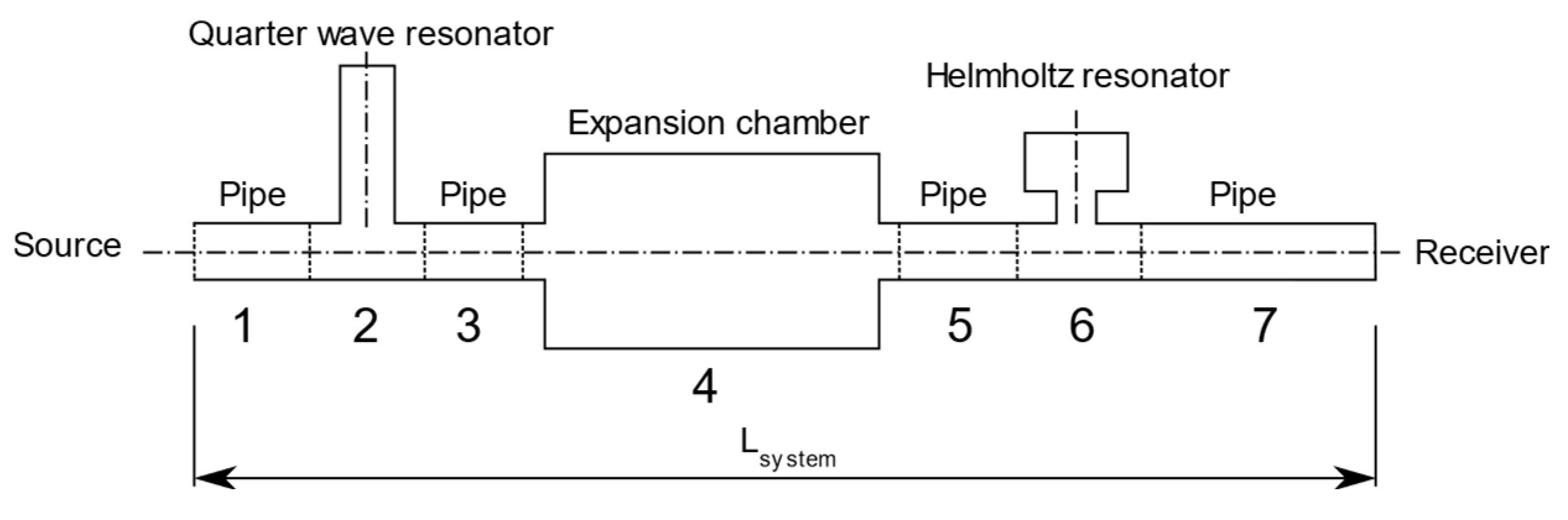
Figure 10.
Example of cascade-coupled silencer system with three silencer elements.

Figure 11.
Simulation of the sound pressure level measured at 0.5 m from the outlet of a 3 m long straight pipe.
Figure 11.
Simulation of the sound pressure level measured at 0.5 m from the outlet of a 3 m long straight pipe.

Figure 12.
TL of the complete system computed using the TMM.

Figure 13.
Sketch of the implementation of the silencer system proposed by the first group. The source is placed at the left side and the outlet at the right side.
Figure 13.
Sketch of the implementation of the silencer system proposed by the first group. The source is placed at the left side and the outlet at the right side.

Figure 14.
Cross section showing an example of the expansion chamber structure.

Figure 15.
Practical implementation of the sketch reported in Figure 14. The source is placed at the right side and the outlet at the left side.
Figure 15.
Practical implementation of the sketch reported in Figure 14. The source is placed at the right side and the outlet at the left side.

Figure 16.
SPL spectra measured at 0.5 m from the outlet for the background noise (blue), 3 m long straight pipe (yellow), and the silencer system (orange).
Figure 16.
SPL spectra measured at 0.5 m from the outlet for the background noise (blue), 3 m long straight pipe (yellow), and the silencer system (orange).

Figure 17.
Comparison between the predicted IL (red) and the measured IL (blue).

Figure 18.
Resulting SPL narrow band and one-third octave band spectra at the receiver. Blue lines: without silencing system. Red lines: with silencing system.
Figure 18.
Resulting SPL narrow band and one-third octave band spectra at the receiver. Blue lines: without silencing system. Red lines: with silencing system.


Table 1.
Example illustrating how the synthesized third octave band spectrum derived from Figure 11 must be modified to achieve an overall SPL lower than 55 dB(A). The numerical value 20 dB is not a requirement on minimum reduction. It is merely an indicator that reduction measures are needed in that band.
| fn [Hz] | LA, Without [dB(A)] | DIL,Necessary [dB] | LA at the Receiver [dB(A)] |
|---|---|---|---|
| 125 | 37.5 | 0 | 24.9 |
| 160 | 38.1 | 0 | 39.5 |
| 200 | 78.2 | 20 | 18.1 |
| 250 | 40.2 | 0 | 40.0 |
| 315 | 41.3 | 0 | 38.9 |
| 400 | 71.3 | 20 | 49.7 |
| 500 | 43.0 | 0 | 35.7 |
| 630 | 66.6 | 20 | 21.5 |
| 800 | 67.5 | 20 | 38.3 |
| 1000 | 64.6 | 20 | 28.9 |
| Total level | 79.7 | 51.2 |
Publisher’s Note: MDPI stays neutral with regard to jurisdictional claims in published maps and institutional affiliations. |
© 2022 by the authors. Licensee MDPI, Basel, Switzerland. This article is an open access article distributed under the terms and conditions of the Creative Commons Attribution (CC BY) license (https://creativecommons.org/licenses/by/4.0/).
Share and Cite
MDPI and ACS Style
Piana, E.A.; Carlsson, U.E.; Lezzi, A.M.; Paderno, D.; Boij, S. Silencer Design for the Control of Low Frequency Noise in Ventilation Ducts. Designs 2022, 6, 37. https://doi.org/10.3390/designs6020037
AMA Style
Piana EA, Carlsson UE, Lezzi AM, Paderno D, Boij S. Silencer Design for the Control of Low Frequency Noise in Ventilation Ducts. Designs. 2022; 6(2):37. https://doi.org/10.3390/designs6020037
Chicago/Turabian StylePiana, Edoardo Alessio, Ulf Erik Carlsson, Adriano Maria Lezzi, Diego Paderno, and Susann Boij. 2022. "Silencer Design for the Control of Low Frequency Noise in Ventilation Ducts" Designs 6, no. 2: 37. https://doi.org/10.3390/designs6020037