
Effects of Load Forecast Deviation on the Specification of Energy Storage Systems
by
 and
and
Alexander Emde
1,2,*,
Lisa Märkle
2,
Benedikt Kratzer
2,
Felix Schnell
1,2,
Lukas Baur
1,2 and
Alexander Sauer
1,2 1
Fraunhofer Institute for Manufacturing Engineering and Automation IPA, 70569 Stuttgart, Germany
2
Institute for Energy-Efficiency in Production, University of Stuttgart, 70569 Stuttgart, Germany
*
Author to whom correspondence should be addressed.
Designs 2023, 7(5), 107; https://doi.org/10.3390/designs7050107
Submission received: 28 July 2023
/
Revised: 30 August 2023
/
Accepted: 7 September 2023
/
Published: 11 September 2023
Abstract
:The liberalization of the German energy market has created opportunities for end-consumers, including industrial companies, to actively participate in the electricity market. By making their energy loads more flexible, consumers can generate additional income and thus save money. Energy storage systems can be utilized to achieve the required flexibility by temporarily storing excess electrical energy in the form of heat, cold, or electricity for later use. This publication focuses on how the dimensionality of energy storage is influenced by load forecasting. The results show that inaccuracies in load forecasting lead to a direct over-dimensioning and thus, a deterioration of the economics of energy storage technologies. Using two scenario cases, it shows on the one hand how important good forecasts are and on the other hand that buffers must be included in the conceptual design in order to be able to compensate for forecast errors.
1. Introduction
1.1. Motivation and Problem Formulation
The implementation of energy storage systems allows industrial companies to reduce their consumption of electricity from the grid, while providing energy independent of grid fluctuations. In addition, the use of energy storage systems enables companies to participate in electricity markets and generate additional revenue. This revenue potential can be a strong incentive for companies to invest in this technology and optimize their energy supply. Zimmermann et al. [1] point out that 37% of the interviewed companies already use energy storages to flexibilize their electricity consumption.
To maximize the monetary value added, it is necessary to size the storage in an economic way as well as to use it in the most efficient way [2,3]. Hence, a high information density and quality is required to maintain the most appropriate use of energy storage systems [4]. The implementation of advanced metering technologies and systems provides the opportunity at brownfield factories to create such a comprehensive database. With today’s technology, companies can gain a comprehensive understanding of their current load profile. However, these advanced metering technologies come at a high initial cost, making them economically unattractive, particularly for energy-intensive industries.
The current installations allow industrial users to get information about their average demand in 15-min intervals. Consumers with an annual consumption of more than 100 MWh are required by law to have a meter reading to determine their individual load profile [5]. Therefore, it is possible to forecast the future demand based on historical data and other available information like the production plan and weather data. These forecasts can also be used to optimize the operating strategy and storage sizing, offering great effectivity potential. In particular, storage sizing plays a key role in the economic use of storage for peak load reduction [6]. Oversizing can only be avoided by a comprehensive data basis and precise load forecast.
Peak shaving can be a lucrative way to save on electricity costs [7]. Using forecasts, peak shaving aims to reduce current load peaks and thus reduce grid charges. The day ahead spot market of the European Power Exchange (EPEX) serves as the central trading place for electricity products, on which hourly and block contracts with physical performance for the following day are traded [8]. The participation in the spot market allows buying electricity during low price periods, while not exceeding the current peak load. On the other hand, the storage will be discharged during peak price periods to maximize the monetary value. By utilizing load forecasts, the previously reactive approach can be changed to a proactive storage control. Due to the increased knowledge from the forecast, it is possible to compare peak loads and current prices and to enable the proactive operation strategy.
1.2. Objective
Since load forecasting is a well-studied problem in literature [9,10,11,12,13,14,15,16,17,18], this paper will focus on how load forecasting and its deviation has an influence on the operational management of the energy storage device. Therefore first the method used to analyze the impact of integrating a forecast on different use cases for grid optimization, is presented. The influencing factors are analyzed and their influence is quantified. Then a forecast is generated and two use cases are planned based on this forecast. Finally, the impact of load forecasting errors on storage sizing is evaluated.
1.3. Scope
The current operation of storages is based on an event control. In the considered example, the energy intensive industry in Germany, if the load is close to exceeding the limitation load in one 15-min interval the storage will be used in the following interval.
A different way to operate energy storage usage will be introduced in this paper. An approach for peak shaving and an approach for participation in the spot market are introduced. Both approaches are based on energy consumption forecasts and validated with a use case of the energy intensive industry consuming more than 100 GWh of electrical energy per year.
The remainder of the paper is structured as follows: Section 2 places the topic in the state of the art. Section 3 describes the method used to answer the research question. In Section 4, this is followed by the evaluation of a data set, followed by a discussion of the results. Section 5 concludes with a summary of the main findings and an outlook.
2. State of the Art
Utilizing forecasts enables the opportunity to optimize complete energy systems. Thus Bartolucci et al. [19] show that by using forecasts in a hybrid renewable energy system the annual operating costs can be reduced by 8.7%, and high discharge currents occur less frequently during a low state of charge (SoC). This leads to a lower stress on the batteries and, thus, to an increased life expectancy [19].
Another example of how forecasts can be used to optimize complete systems is given by Jia et al. [20]. In hydrogen fuel cell hybrid electric vehicles, the integration of a novel energy management strategy, including speed prediction, can reduce the battery aging rate by 34.8% and the total cost of ownership by 12.3% [20].
However, for the best use of storage systems, precise load forecasts are needed. Overall forecasts are divided into long-term, medium-term and short-term predictions based on the forecast horizon [21]. Long-term forecasts are created up to one year in advance, while short-term methods are prepared several hours up to one week in advance [21,22]. Hence, medium-term forecasts fill the gap between the long- and short-term forecasts. Additionally, the forecast methods can be categorized into three categories of forecasts, the classical method, methods of artificial intelligence and reference-based methods [22].
A common classical method is regression. This method shows statistical links between energy consumption and other factors [23]. Using historical data, a regression coefficient is calculated which maps the correlation between load and other variables of the factory [21]. The reference-based method uses certain reference values as forecasts. In the comparison to the day method historical data of a certain day with repeating characteristics, such as the same weekday or the same time, is used as a forecast [21].
The regression method and the reference-based method refer to various parameters that determine the actual energy demand. Climate factors, seasonal influences and operating parameters are taken into account for the forecast. Exemplary climate factors are the temperature, the wind speed or the global solar radiation. Seasonal influences are weekdays, the season or special days, like holidays. Operating parameters could be the location, the load factor or the production plan.
Forecast models based on a combination of the regression and the comparison date method are able to guarantee a high forecasting quality. The forecast quality can be measured by the Mean Absolute Percentage Error (MAPE) metric [24]. It was chosen because of its property that it makes statements about the quality independent of the absolute load and is a frequently used metric in the literature [25,26,27].
The MAPE calculates the accuracy as a percentage and determines the deviation of the actual value yt from the forecast value ŷt for each time period:
For the comparison of a single data point the MAPE reduces to the relative error. This metric is useful for describing the change of errors over time. A precise load forecast is becoming increasingly important for commercial and industrial companies in order to be able to identify the possible load shift potential at an early stage. Only by recognizing the potential for load shifting can appropriate measures be taken to reduce peak loads [28,29,30]. Further improvements in the forecasting quality are therefore desirable. This can be achieved by using artificial intelligence methods such as artificial neural networks, fuzzy methods or adaptive logical networks. These are able to learn complex non-linear relationships and are therefore less susceptible to uncertainties and inaccurate input variables [27]. Afrasiabi et al. [31] and Zor et al. [32] present results which show that a forecast based on deep learning is 50% more precise compared to other forecast methods.
The load analysis methodology described by Emde et al. [33] allows a detailed insight into the composition of the load and its dependence on external factors. This method provides a basis for accurate predictions. Both the thermal and the electrical load of an industrial company were examined to determine the correlating factors. The method does not only require a representative database of load profiles, but also data on influencing factors, such as weather and time-dependent production data.
There have been many different studies in the field of energy storage in combination with load forecasting [34,35,36]. For instance, Hwang et al. [37] investigate the extent to which peak power can be reduced by using energy storage in a real building, and how the energy storage systems can be optimally scheduled to achieve this. Besides Chapaloglou et al. [38] use a feedforward artificial neural network, capable of short-term, day ahead load forecasting for load smoothing and peak shaving of an island’s power system in combination with a battery energy storage system. Collath et al. [39] developed an operation strategy to reduce battery degradation during peak shaving elicited by forecast errors. In addition, Ilic et al. [40] are investigating how energy storage systems need to be dimensioned in a smart grid to compensate for forecast errors. Conversely, however, the consequences of load forecasting inaccuracies on the sizing of energy storage systems have not yet been considered and are the subject of this paper.
3. Methodology
The method used to analyze the impact of integrating a forecast on different use cases for grid optimization, is presented in detail below. First, influencing factors on the load forecast are analyzed by a correlation analysis and their influences are quantified. Then a forecast is generated and trained with load profiles of an industrial company from the automotive sector. Based on the developed load forecast the storage is sized for two different use cases, described in Section 3.3 (see Figure 1).
3.1. Correlation Analysis
In a first step, a correlation analysis of the electrical and cooling load profiles of a reference year is carried out. Therefore, the load profiles for type weeks corresponding to the seasons of summer, winter and transitional period (autumn and spring) are examined and characteristic correlated variables are identified. The used load profiles are from an industrial company from the automotive sector producing in a two-shift operation. Over the whole year, the average electrical power consumption is around 30 kW and the standard deviation of the load profile is slightly above 10 kW.
In addition to seasonal differences, it is also possible to identify differences in the load curve between working days and weekends. For clarification, Figure 2 compares the relative electrical load (related to the peak load) with the temperature. It is noticeable that the load points can be divided into two groups, working days and weekends (linear regression: coefficient of determination R2 [41] is 0.41 for working days and 0.37 for weekends). The differences in the load curve between working days and weekends are due to changes in the production load within the company. The strong influence of the outside temperature is particularly visible in the cooling consumption (which is generated by electrical energy) during working days, with an increase in temperature also leading to an increase in electrical energy consumption. The electrical peak load occurred on a Monday afternoon, outside the company holidays, at an ambient temperature of 33 °C. This correlation between the temperature and the electrical energy consumption is particularly evident in summer due to the increased cooling demand and the resulting higher electrical load. During winter period there is a lower correlation between the load and the outside temperature. The correlation between the electrical load and the temperature can be observed both on working days and on weekends. However, the slope of the electrical load with the temperature increase is greater on working days than on weekends. There are some outliers between the weekday and weekend data points, reflecting, for example, half working days such as Fridays, or days with low production utilization. In addition, the outliers may be caused by factors other than the type of day, which are examined in Table 1.
Table 1 shows the examined parameters of thermal and electrical load and their relevance. The parameters are compared by using correlation analysis by calculating the correlation coefficient R [42]. Parameters with high influence are marked with +++ (|R| > 0.9), while parameters with medium influence are marked with ++ (0.5 ≤ |R| ≤ 0.9), and parameters with low influence are marked with + (|R| < 0.5). On the one hand, the statistics show that the electrical load depends on the outside temperature, the production data and the day of the week. The thermal load, on the other hand, is highly dependent on the outside temperature, especially for temperatures above 15 °C. The load forecast is carried out on the basis of the environmental temperature, the production times and the day of the week.
3.2. Forecasting Model Based on the Correlation Analysis
In order to study the forecasting errors in storage dimensioning, a forecast is required. A method is presented below as an example. It uses a combination of multiple linear regression and the comparison day method to calculate a day-ahead prediction on a 15-min scale. It is briefly described in the following.
The model uses a multiple linear regression approach on the temperature prediction of that day called T and the production plan data P to predict the 96 forecast vector entries (15 min steps resulting in 96 data points each day), as shown in Figure 3. As Table 1 shows, these two parameters, the temperature and the production plan, have the greatest influence on the loads. The forecast consists of the concatenation of four sub-forecasts, each covering a 6 h block (one shift). The coefficients of the regression (a, b, c), which can vary from day to day, are taken from the coefficient fit of a corresponding reference day. The reference days are defined as follows: For Tuesday through Friday, the reference day is the previous day in each case. For the parameters of a Monday, the previous Monday of the week before is used. Finally, the loads of the reference days are multiplied by the regression coefficients and the forecasted load is obtained.
To evaluate the accuracy of the developed forecasting model, a naïve load forecast is used. In the naïve forecast, the previous value is assumed for the test forecast value [43]. Applied to this use case, the naïve forecast uses the previous day as the forecast for the next day. Again, the previous day is assumed as the reference day for Tuesday to Friday. For the loads of a Monday, the previous Friday is used again.
3.3. Use Cases: Energy Storage Sizing and Operation Planning
The weekly forecast will then be used to size the energy storage unit and plan its operation. Two scenarios for the application of the energy storage device are examined.
The first scenario is an operation strategy for the storage unit in order to reduce the overall grid load (peak shaving). Based on the forecast the storage is discharged to reduce the peak loads. In a subsequent step, a comparison with the actual load is made to determine whether the forecast overestimates or underestimates the amount of energy and the amplitude of the load peaks and how these affect the actually required performance operation of the storage system.
In a second scenario, the storage will be charged and discharged based on price signals of the day-ahead spot market. Low price signals start the charging process of the storage unit. The load forecast provides assistance to the company to plan an electricity purchase on the next day in order to charge the storage facility without running the risk of increasing the maximum load.
In the following, the extent to which the dimensioning of the storage technologies used is influenced by inaccuracies in the forecasting model used or their performance is reduced is examined for both scenarios.
4. Results and Discussion
4.1. Forecast Analysis
Figure 4 shows the loads of a forecasted summer week by the developed load forecast strategy in blue and the actual load in red. The electrical load was predicted using the method from Section 3.2.
In Comparison to the developed load forecast, Figure 5 shows the same forecasted summer week but by the naïve load forecast in green and the actual load in red. As described above, the naïve forecast uses only the loads of the day before as the prediction.
Furthermore, in Figure 6, a comparison of the relative errors of the developed and the naïve load forecast is shown. Within the shown working days, the relative errors of the developed load forecast is on average around three to five percent while the relative errors of the naïve load forecast is between three to ten. Especially the Monday and the Friday are much worse predicted by the naïve load forecast. For the whole datasets, the developed load forecast, having a MAPE of 2.88%, outperforms the naïve load forecast having a MAPE of 4.32% Here, the forecasts of the developed load forecast were much more accurate. This is due to the fact that the production schedule on Mondays, which is much more utilized than on Fridays, is included in the developed load forecast and thus the load demand can be better predicted. On the other days (Tuesday to Thursday), however, the load forecast can only be improved slightly. It is shown that peak loads and minimum loads are predicted for most of the profiles studied by the developed load forecast, but even if the predictions are more accurate than with the naïve load forecast, their characteristics differ from the actual load. These deviations can be explained by unpredictable events, such as system breakdowns, temperature changes or the temporary operation of additional machines. The significant increase in the relative error even of the developed forecast on Friday afternoon to over 20% may be explained by the fact that employees may have finished their workday earlier than scheduled in the underlying shift model, resulting in the actual load decreasing faster than the load forecast. Later in the evening, the load forecast is more in line with the actual load, so the relative error decreases again.
4.2. Impact on Peak Load Reduction
As shown, the forecast is not completely accurate (but more precise than the naïve load forecast). This leads to problems in the peak shaving scenarios, because any peak, which is not correctly forecasted, will not be shaved the way it is supposed to. Consequently, the storage technologies used would have to be dimensioned larger in order to shave not forecasted peaks with some kind of residual storage level. To address this issue, an analysis is conducted to examine the performance of the peak shaving process based on the developed load forecasting model. Figure 7 shows the storage load for the peak shaving scenario with a peak load minimization of 1 MW. The storage is charged and discharged according to the forecast. When the predicted load exceeds the load limit (pl), the storage system is discharged. However, peaks that exceed the green line in Figure 7 are not predicted by the forecast, leading to potential issues in peak shaving.
Figure 8 shows the actual load without storage operation, the residual load of the actual load in combination with a storage operating based on the developed load forecast and the residual load with complete information on the load. It also shows the desired shave level (pl), the actual shave level (pa) and the maximum load (pm) before peak shaving. The violet line displays the deviation of the residual load with perfect storage management and the residual load with storage operation based on the forecast. A positive deviation means that the actual load is underestimated. This causes peak loads to be reduced only partially or not at all. Accordingly, a negative deviation means an overestimation of the load and leads to a reduction of peak loads, which do not actually have to be reduced. In Figure 9, the shaving of Tuesday is shown. It can be seen, that one peak is not forecasted correctly by the developed forecasting model. At 15:00 o’clock, the electrical load was underestimated by the forecast so the storage was not charged enough to shave the peak load according to the desired shave level. As a result, the desired shave level is exceeded. In this scenario, 2.2% of the electrical load peak should be shaved to maintain the desired shave level. Instead, only 1.3% of the electrical peak was shaved. For this reason, the actual peak load is higher than the desired peak load.
The same was carried out up to a peak shave of 3 MW. The results are displayed in Table 2. It can be seen, that the deviation rises with increasing load reduction. One reason is that new peaks will be generated by charging the storage when a low load is predicted.
However, the actual power cut is achieved by using a predefined offset, which guarantees a successful peak shaving. In order to find the right amplitude for the offset the deviation between actual load and forecast is analyzed. The results of this analysis are displayed in Table 3.
Ensuring that the storage is able to cut the peaks at all times the offset has to be the maximum deviation. Therefore, the storage is oversized and leads to a higher capital expenditure. For a better understanding of the results, another analysis focusing at the storage sizes for different peak shave scenarios is conducted. These results are displayed in Table 4.
Table 4 shows that the oversized capacity is negatively correlating with the cut power peak. To reduce the actual load by 1 MW the storage would have to be four times the power and five times the sized capacity. If the storage should cut only 2500 kW the power and capacity is oversized approximately two times compared to the peak power cut based on the actual load. A possible explanation is the choice of offset. Since the offset must be the maximum power to make sure the load is not exceeded, the oversizing ratio will become smaller with larger storages.
It is shown, that in order to conduct peak shaving the storages based on the forecast, respectively the forecast combined with an offset, need to be oversized. This leads to a weakened economic performance. The reason for an oversized capacity is based on the fact that the forecast allows the storage to be charged during times where the actual load is above the maximum load. Using the offset requires greater capacity and power, resulting in increased storage costs. A potential solution for this problem is charging at night. However, considering this option the capacity is even increased and not decreased.
4.3. Impact on Spot Market Revenue
Another application of load forecasting is the determination of charging and discharging times when participating in the spot market to take advantage of volatile prices. Here, the developed forecast is used to optimize the operation strategy of a storage, which participates in the spot market without exceeding the current load limit. Figure 10, Figure 11 and Figure 12 show the differences with respect to the storage business case. In all scenarios, there is a given maximum load, which should not be exceeded (purple line). This maximum is the peak load of the actual load. Furthermore, the spot market prices are plotted in the Figure 10, Figure 11 and Figure 12. Apart from minor changes, the course of the price over the different days of the week is reproducible, similar to the load course.
With complete data of the current load, it would be possible to charge the storage, whenever the load is below the load limit and the price is below the average market price. As shown in Figure 10, this would allow charging the storage in the morning hours as well as some times during the day.
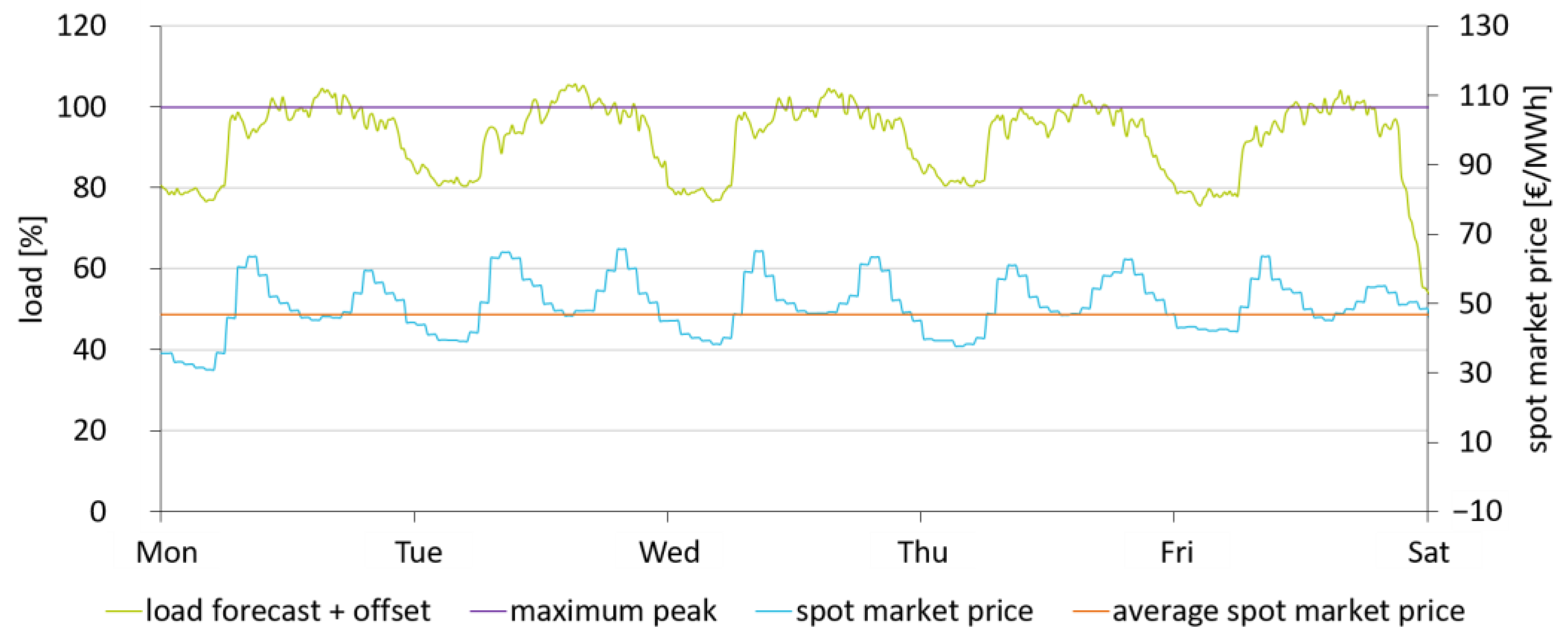
In Figure 11, the forecast is displayed and is constantly below the load limit. This would reduce the restrictions to just the monetary aspect. Whenever the price is below average, the storage is charged and whenever the price is above the average, the storage is discharged. This strategy exceeds the load limit in the actual load. Hence, it is necessary to add an offset to ensure not exceeding the load limit. This is shown in Figure 12 and allows charging the storage whenever the forecast with offset is below the maximum load and the price is below the average price.
If we consider both the times when the spot market prices are below the average and the times when the forecast with offset is below the maximum load, we can see that the storage units can only be charged in the morning hours of the respective day. Once the electrical storage has been charged in the morning, it is discharged during the rest of the day according to the occurring load peaks that occur, until it can be charged again the next morning. In this way, it is possible to take advantage of the favorable energy prices of the spot market and at the same time shaving the electrical peak loads.
Based on Figure 10, Figure 11 and Figure 12 an analysis of the storage’s performance on the spot market is conducted.
Table 5 shows the calculation results for an exemplary storage application and its potential annual revenue. The storage power is 1 MW power and has a capacity of 1 MWh, so it can easily be scaled upwards or downwards. These calculations may vary for each load and its respective forecast, but show a use case for energy storage devices.
The revenue is maximized for an operation strategy based on the actual load is the highest. However, it also exceeds the actual load limit by 250 kW, which leads to additional cost. As the price for 1 kW is 68.40 € the total added cost is 17,100 € [44]. The operating strategy, which allows the storage to be charged only at night, offers the lowest potential revenue of 201,292 €. This is due to some missed charging windows during the day and the high price in the evening. Hence, the charging aim based on the forecast and offset is to achieve a higher potential revenue, while maintaining the current peaks and not exceeding the maximum load. Therefore, the forecast is offering an opportunity to maximize the revenues on the spot market without causing additional costs. With a potential annual revenue of 251,420 € this scenario almost reaches the annual revenue potential of charging the storage based on the actual load with 266,656 €. The opportunity to charge during the day and before a price peak is possible, but not considered in this scenario. This is due to the high priority given to ensuring that the maximum load is not exceeded. The main goal is still to reduce peak loads.
5. Conclusions and Outlook
As can be seen from the results, in the peak shaving scenario even small deviations from the actual load lead to a much higher capacity and performance of the storage system and therefore lead to much higher costs. This shows once again how important precise load forecasting is for peak shaving and the dimensioning of storage systems. Moreover, it can be seen that to reduce the intended load peaks, an offset must be applied. This results in an additional increase of the required storage capacity, so no new load peak arises. Based on the load forecast, it is however possible to generate savings on the day ahead market by using a storage device.
In summary, the prediction of energy consumption in energy-intensive industries is feasible. Moreover, this forecast can be used for peak shaving purposes, but there is still room for improvement to ensure an efficient utilization process. Any peak that is not correctly forecasted will not be shaved the way it is supposed to. Consequently, the load forecast precise must be increased or the storage technologies would have to be oversized. In numerical therms, the oversized capacity is negatively correlating with the cut power peak. As shown to reduce the actual load by 1 MW the storage would be four times the power, while cutting only 2500 kW the power and capacity is only two times the peak power cut based on the actual load. As discussed the choice of offset is a possible explanation. Further investigation should focus on the best choice of offset for peak load reduction. Among the two applications explored, participation in the spot market seems to be the most promising. As shown the use of an appropriate load forecast can help to exploit the low price times of the spot market price. However, it is important to ensure that storage charging does not lead to new peak loads. As shown, this can be ensured by using a load forecast. Overall, this paper has shown that in both cases considered, the sizing of the storage increased sharply with the inaccuracy of the load forecast. As a result, the costs of the storage systems increased, not always leading to higher potential revenues, meaning that the economic operation of the energy storage system is closely related to the quality of the load forecast and the size of the offset. Consequently, future studies should create better load forecasting models, which was not a focus of this paper. The forecasting methodology developed is based on historical reference data and correlations. However, if circumstances or dependencies change on the day being forecasted, these cannot be considered, resulting in larger forecast deviations. It can be seen that even small deviations in the load forecast have a major impact on the effectiveness and economic efficiency of the electrical storage system used for peak shaving. The development of even more accurate prediction models will therefore be necessary in the future. A possible next step would be to investigate whether a neural network-based forecast could lead to predictions that are even more accurate. In addition, it would be worth investigating what other benefits an artificial intelligence-based prediction would bring. Once these future investigations are completed, storage technologies can be used even more efficiently, improving the economic and environmental benefits for industrial companies.
Author Contributions
Investigation A.E.; Project administration A.E.; Conceptualization, L.M.; data curation, L.M.; methodology L.M.; writing—original draft preparation, B.K.; writing review and editing, F.S. and L.B.; supervision A.E. and A.S. All authors have read and agreed to the published version of the manuscript.
Funding
This research was funded by Federal Ministry of Education and Research (BMBF) grant number [03SFK3Q2-2].
Data Availability Statement
3rd Party Data. Restrictions apply to the availability of these data. Data was obtained from an industrial company and are available from the authors with the permission of the industrial company.
Acknowledgments
The authors would like to thank the BMBF and Project Management Jülich, who supported and supervised the Synergie research project.
Conflicts of Interest
Hereby the authors declare that they have no conflict of interest.
References
- Zimmermann, F.; Emde, A.; Laribi, R.; Wang, D.; Sauer, A. Energiespeicher in Produktionssystemen—ESIP Studie. Herausforderungen und Chancen; University of Stuttgart: Stuttgart, Germany, 2019. [Google Scholar] [CrossRef]
- Elio, J.; Peinado-Guerrero, M.; Villalobos, R.; Milcarek, R.J. An energy storage dispatch optimization for demand-side management in industrial facilities. J. Energy Storage 2022, 53, 105063. [Google Scholar] [CrossRef]
- Carpinelli, G.; Di Fazio, A.; Khormali, S.; Mottola, F. Optimal Sizing of Battery Storage Systems for Industrial Applications when Uncertainties Exist. Energies 2014, 7, 130–149. [Google Scholar] [CrossRef]
- Hannan, M.A.; Faisal, M.; Jern Ker, P.; Begum, R.A.; Dong, Z.Y.; Zhang, C. Review of optimal methods and algorithms for sizing energy storage systems to achieve decarbonization in microgrid applications. Renew. Sustain. Energy Rev. 2020, 131, 110022. [Google Scholar] [CrossRef]
- Bitterer, R.; Schieferdecker, B. Repräsentative VDEW-Lastprofile; Technical Report; Verband der Elektrizitätswirtschaft e. V. (VDEW): Frankfurt, Germany, 1999. [Google Scholar]
- Zimmermann, F.; Pottmeier, D.; Emde, A.; Sauer, A. A Comparison of Peak Shaving and Atypical Grid Usage Application for Energy Storage Systems in the German Industrial Sector. In Proceedings of the EnInnov2020: 16, Symposium Energieinnovation Energy for Future—Wege zur Klimaneutralität, Graz, Austria, 12–14 February 2020; Technische Universität Graz: Graz, Austria, 2020; pp. 303–304. [Google Scholar]
- Yesilyurt, O.; Bauer, D.; Emde, A.; Sauer, A. Why should the automated guided vehicles’ batteries be used in the manufacturing plants as an energy storage? E3S Web Conf. 2021, 231, 01004. [Google Scholar] [CrossRef]
- Viehmann, J. State of the German Short-Term Power Market. Z. Energiewirtschaft 2017, 41, 87–103. [Google Scholar] [CrossRef]
- Kim, Y.; Son, H.; Kim, S. Short term electricity load forecasting for institutional buildings. Energy Rep. 2019, 5, 1270–1280. [Google Scholar] [CrossRef]
- Ryu, S.; Noh, J.; Kim, H. Deep Neural Network Based Demand Side Short Term Load Forecasting. Energies 2017, 10, 3. [Google Scholar] [CrossRef]
- Khan, A.R.; Mahmood, A.; Safdar, A.; Khan, Z.A.; Khan, N.A. Load forecasting, dynamic pricing and DSM in smart grid: A review. Renew. Sustain. Energy Rev. 2016, 54, 1311–1322. [Google Scholar] [CrossRef]
- Ghasemi, A.; Shayeghi, H.; Moradzadeh, M.; Nooshyar, M. A novel hybrid algorithm for electricity price and load forecasting in smart grids with demand-side management. Appl. Energy 2016, 177, 40–59. [Google Scholar] [CrossRef]
- Zheng, J.; Xu, C.; Zhang, Z.; Li, X. Electric load forecasting in smart grids using Long-Short-Term-Memory based Recurrent Neural Network. In Proceedings of the 2017 51st Annual Conference on Information Sciences and Systems (CISS), Baltimore, MD, USA, 22–24 March 2017; IEEE: Piscataway, NJ, USA, 2017; pp. 1–6, ISBN 978-1-5090-4780-2. [Google Scholar]
- Hippert, H.S.; Pedreira, C.E.; Souza, R.C. Neural networks for short-term load forecasting: A review and evaluation. IEEE Trans. Power Syst. 2001, 16, 44–55. [Google Scholar] [CrossRef]
- Dewangan, F.; Abdelaziz, A.Y.; Biswal, M. Load Forecasting Models in Smart Grid Using Smart Meter Information: A Review. Energies 2023, 16, 1404. [Google Scholar] [CrossRef]
- Habbak, H.; Mahmoud, M.; Metwally, K.; Fouda, M.M.; Ibrahem, M.I. Load Forecasting Techniques and Their Applications in Smart Grids. Energies 2023, 16, 1480. [Google Scholar] [CrossRef]
- Wang, H.; Alattas, K.A.; Mohammadzadeh, A.; Sabzalian, M.H.; Aly, A.A.; Mosavi, A. Comprehensive review of load forecasting with emphasis on intelligent computing approaches. Energy Rep. 2022, 8, 13189–13198. [Google Scholar] [CrossRef]
- Zhu, J.; Dong, H.; Zheng, W.; Li, S.; Huang, Y.; Xi, L. Review and prospect of data-driven techniques for load forecasting in integrated energy systems. Appl. Energy 2022, 321, 119269. [Google Scholar] [CrossRef]
- Bartolucci, L.; Cordiner, S.; Mulone, V.; Santarelli, M. Hybrid renewable energy systems: Influence of short term forecasting on model predictive control performance. Energy 2019, 172, 997–1004. [Google Scholar] [CrossRef]
- Jia, C.; Zhou, J.; He, H.; Li, J.; Wei, Z.; Li, K.; Shi, M. A novel energy management strategy for hybrid electric bus with fuel cell health and battery thermal- and health-constrained awareness. Energy 2023, 271, 127105. [Google Scholar] [CrossRef]
- Schellong, W. Analyse und Optimierung von Energieverbundsystemen, 1. Auflage; Springer: Berlin/Heidelberg, Germany, 2016; ISBN 978-3-662-49463-9. [Google Scholar]
- Hirsch, C. Fahrplanbasiertes Energiemanagementsystem in Smart Grids; KIT: Karlsruhe, Germany, 2017. [Google Scholar]
- Chow, J.H.; Wu, F.F.; Momoh, J. Applied Mathematics for Restructured Electric Power Systems: Optimization, Control, and Computational Intelligence; Springer: Boston, MA, USA, 2005; ISBN 978-0-387-23471-7. [Google Scholar]
- Chen, K. Trends in Neural Computation; Springer: Berlin/Heidelberg, Germany, 2007; ISBN 978-3-540-36122-0. [Google Scholar]
- Almeshaiei, E.; Soltan, H. A methodology for Electric Power Load Forecasting. Alex. Eng. J. 2011, 50, 137–144. [Google Scholar] [CrossRef]
- Nti, I.K.; Teimeh, M.; Nyarko-Boateng, O.; Adekoya, A.F. Electricity load forecasting: A systematic review. J. Electr. Syst. Inf. Technol. 2020, 7, 13. [Google Scholar] [CrossRef]
- Hahn, H.; Meyer-Nieberg, S.; Pickl, S. Electric load forecasting methods: Tools for decision making. Eur. J. Oper. Res. 2009, 199, 902–907. [Google Scholar] [CrossRef]
- Chen, C.; Duan, S.; Cai, T.; Liu, B.; Hu, G. Optimal Allocation and Economic Analysis of Energy Storage System in Microgrids. IEEE Trans. Power Electron. 2011, 26, 2762–2773. [Google Scholar] [CrossRef]
- Soroudi, A.; Siano, P.; Keane, A. Optimal DR and ESS Scheduling for Distribution Losses Payments Minimization under Electricity Price Uncertainty. IEEE Trans. Smart Grid 2016, 7, 261–272. [Google Scholar] [CrossRef]
- Mukhopadhyay, P.; Mitra, G.; Banerjee, S.; Mukherjee, G. Electricity load forecasting using fuzzy logic: Short term load forecasting factoring weather parameter. In Proceedings of the 2017 7th International Conference on Power Systems (ICPS), Pune, India, 21–23 December 2017; IEEE: Piscataway, NJ, USA, 2017; pp. 812–819, ISBN 978-1-5386-1789-2. [Google Scholar]
- Afrasiabi, M.; Mohammadi, M.; Rastegar, M.; Kargarian, A. Multi-agent microgrid energy management based on deep learning forecaster. Energy 2019, 186, 115873. [Google Scholar] [CrossRef]
- Zor, K.; Timur, O.; Teke, A. A state-of-the-art review of artificial intelligence techniques for short-term electric load forecasting. In Proceedings of the 6th International Youth Conference on Energy (IYCE), Budapest, Hungary, 21–24 June 2017; IEEE: Piscataway, NJ, USA, 2017; pp. 1–7, ISBN 978-1-5090-6409-0. [Google Scholar]
- Emde, A.; Zimmermann, F.; Feil, M.; Sauer, A. Erstellung und Validierung von Lastprofilen für die energieintensive Industrie. Z. Wirtsch. Fabr. 2018, 113, 545–549. [Google Scholar] [CrossRef]
- Dutta, S.; Sharma, R. Optimal storage sizing for integrating wind and load forecast uncertainties. In Proceedings of the 2012 IEEE PES Innovative Smart Grid Technologies (ISGT), Washington, DC, USA, 16–20 January 2012; pp. 1–7, ISBN 978-1-4577-2159-5. [Google Scholar]
- Senchilo, N.D.; Ustinov, D.A. Method for Determining the Optimal Capacity of Energy Storage Systems with a Long-Term Forecast of Power Consumption. Energies 2021, 14, 7098. [Google Scholar] [CrossRef]
- Soman, A.; Trivedi, A.; Irwin, D.; Kosanovic, B.; McDaniel, B.; Shenoy, P. Peak Forecasting for Battery-based Energy Optimizations in Campus Microgrids. In Proceedings of the Eleventh ACM International Conference on Future Energy Systems, Virtual Event, Australia, 22–26 June 2020; ACM: New York, NY, USA, 2020; pp. 237–241, ISBN 9781450380096. [Google Scholar]
- Hwang, J.S.; Rosyiana Fitri, I.; Kim, J.-S.; Song, H. Optimal ESS Scheduling for Peak Shaving of Building Energy Using Accuracy-Enhanced Load Forecast. Energies 2020, 13, 5633. [Google Scholar] [CrossRef]
- Chapaloglou, S.; Nesiadis, A.; Iliadis, P.; Atsonios, K.; Nikolopoulos, N.; Grammelis, P.; Yiakopoulos, C.; Antoniadis, I.; Kakaras, E. Smart energy management algorithm for load smoothing and peak shaving based on load forecasting of an island’s power system. Appl. Energy 2019, 238, 627–642. [Google Scholar] [CrossRef]
- Collath, N.; Englberger, S.; Jossen, A.; Hesse, H. Reduction of Battery Energy Storage Degradation in Peak Shaving Operation through Load Forecast Dependent Energy Management. In Proceedings of the NEIS 2020: Conference on Sustainable Energy Supply and Energy Storage Systems, Hamburg, Germany, 14–15 September 2020; Schulz, D., Ed.; VDE VERLAG: Berlin, Germany, 2020; pp. 1–6, ISBN 978-3-8007-5359-8. [Google Scholar]
- Ilic, D.; Karnouskos, S.; Goncalves Da Silva, P. Improving Load Forecast in Prosumer Clusters by Varying Energy Storage Size. In Proceedings of the IEEE Grenoble PowerTech, Grenoble, France, 16–20 June 2013. [Google Scholar]
- Quinino, R.C.; Reis, E.A.; Bessegato, L.F. Using the coefficient of determination R2 to test the significance of multiple linear regression. Teach. Stat. 2013, 35, 84–88. [Google Scholar] [CrossRef]
- Asuero, A.G.; Sayago, A.; González, A.G. The Correlation Coefficient: An Overview. Crit. Rev. Anal. Chem. 2006, 36, 41–59. [Google Scholar] [CrossRef]
- Hyndman, R.J.; Athanasopoulos, G. Forecasting: Principles and Practice, 2nd ed.; Otexts Online Open-Access Textbook; Otexts: Lexington, KY, USA, 2018; ISBN 978-0-9875071-1-2. [Google Scholar]
- Elektrizitätswerk Hammermühle. Preisblatt für die Netznutzung des Stromnetzes der EWH Versorgungs GmbH; Elektrizitätswerk Hammermühle: Selters, Germany, 2017. [Google Scholar]
Figure 1.
Storage sizing approach based on load forecasting.

Figure 2.
Correlation between outside temperature and electrical load. The load was normalized based on the annual peak load. For clarity, only 3 weeks of data were plotted.
Figure 2.
Correlation between outside temperature and electrical load. The load was normalized based on the annual peak load. For clarity, only 3 weeks of data were plotted.
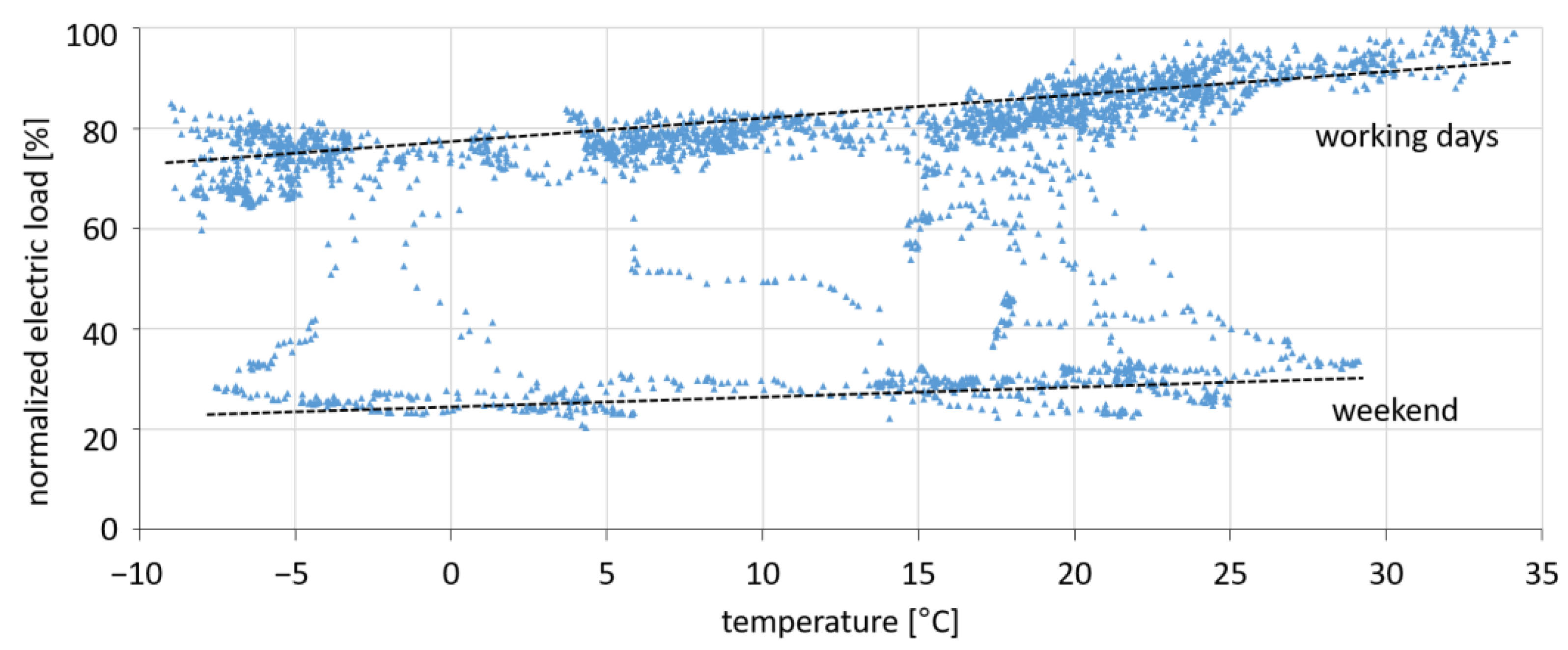
Figure 3.
Forecasting strategy based on the correlation analysis from Section 3.2.
Figure 3.
Forecasting strategy based on the correlation analysis from Section 3.2.
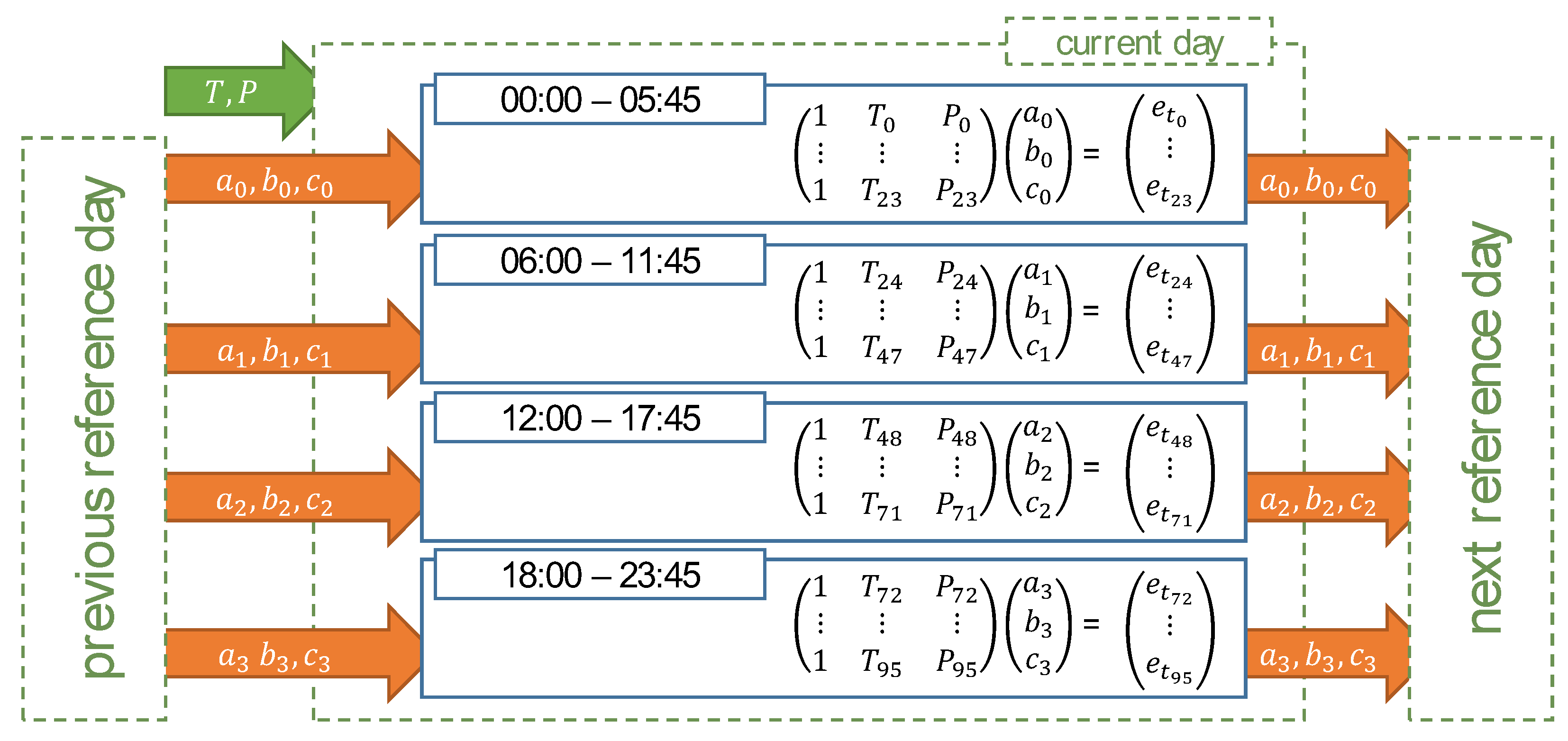
Figure 4.
Developed load forecast and actual load with the corresponding relative errors.
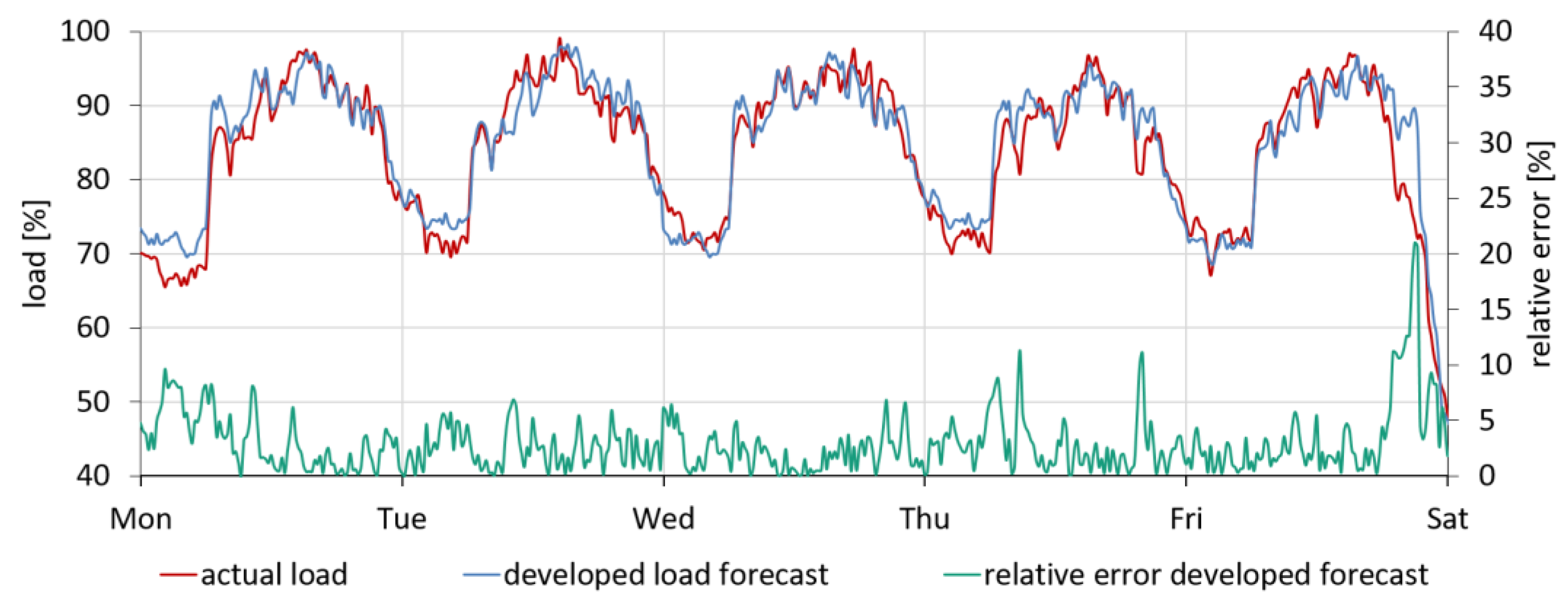
Figure 5.
Naïve load forecast and actual load with the corresponding relative errors.
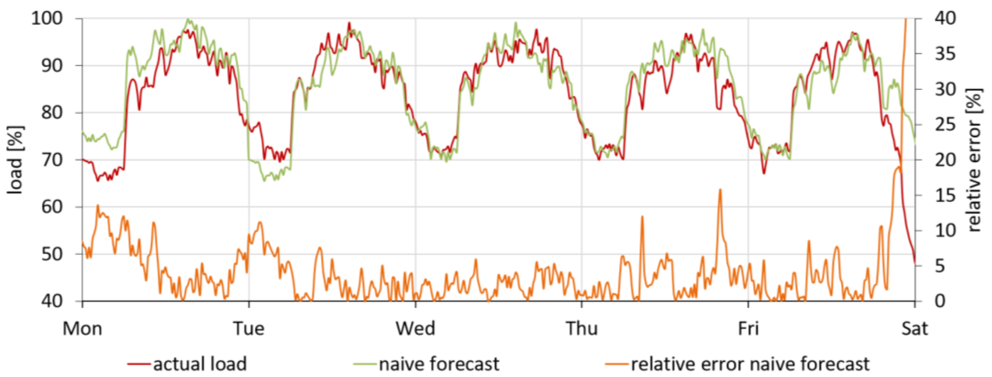
Figure 6.
Comparison of the relative errors of the load forecasts over time.

Figure 7.
Peak shaving with forecast and actual peak shaving.
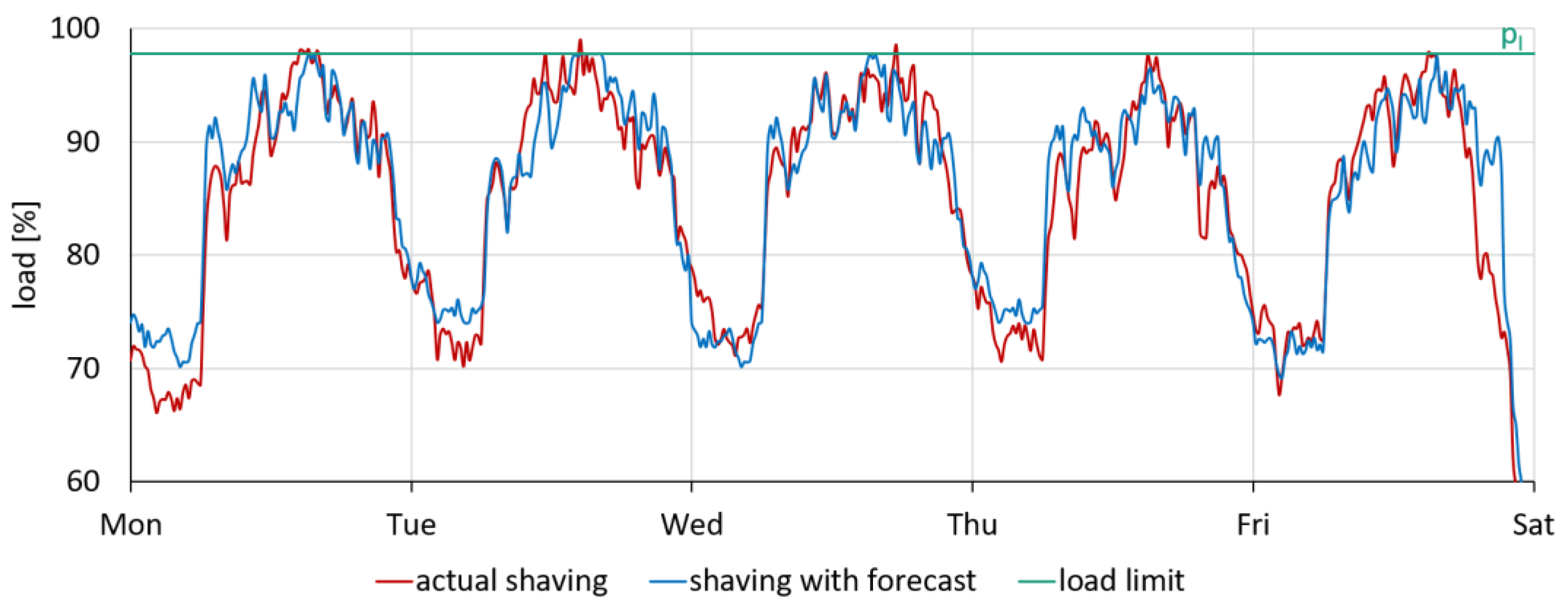
Figure 8.
Residual load with 1 MW peak shaving.
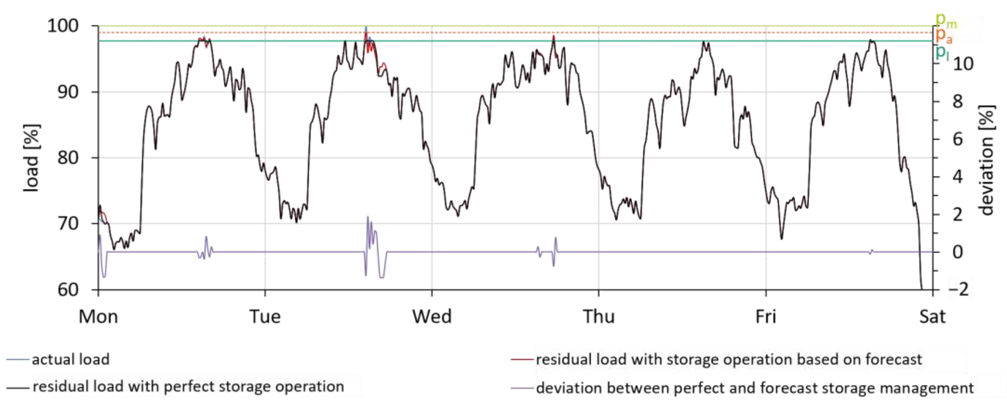
Figure 9.
More detailed look on the residual load with 1 MW peak shaving on Tuesday.
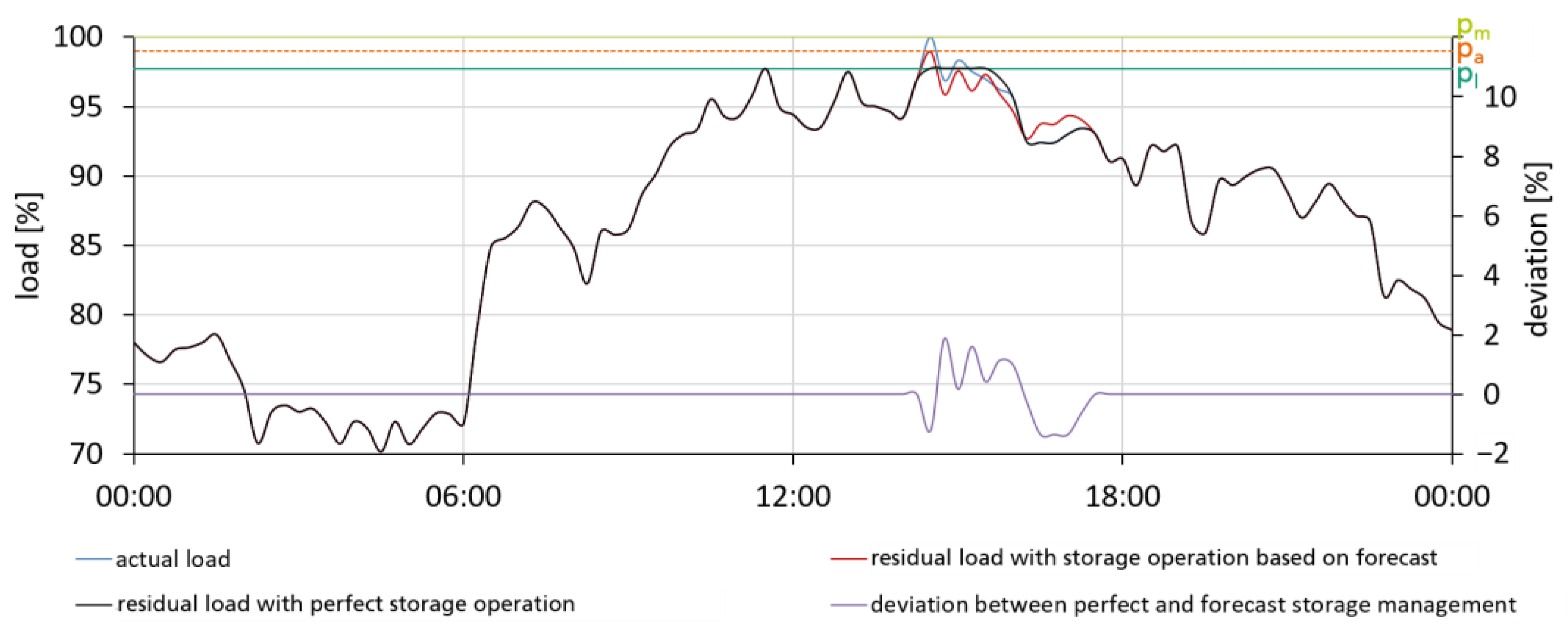
Figure 10.
Actual load and spot market prices.
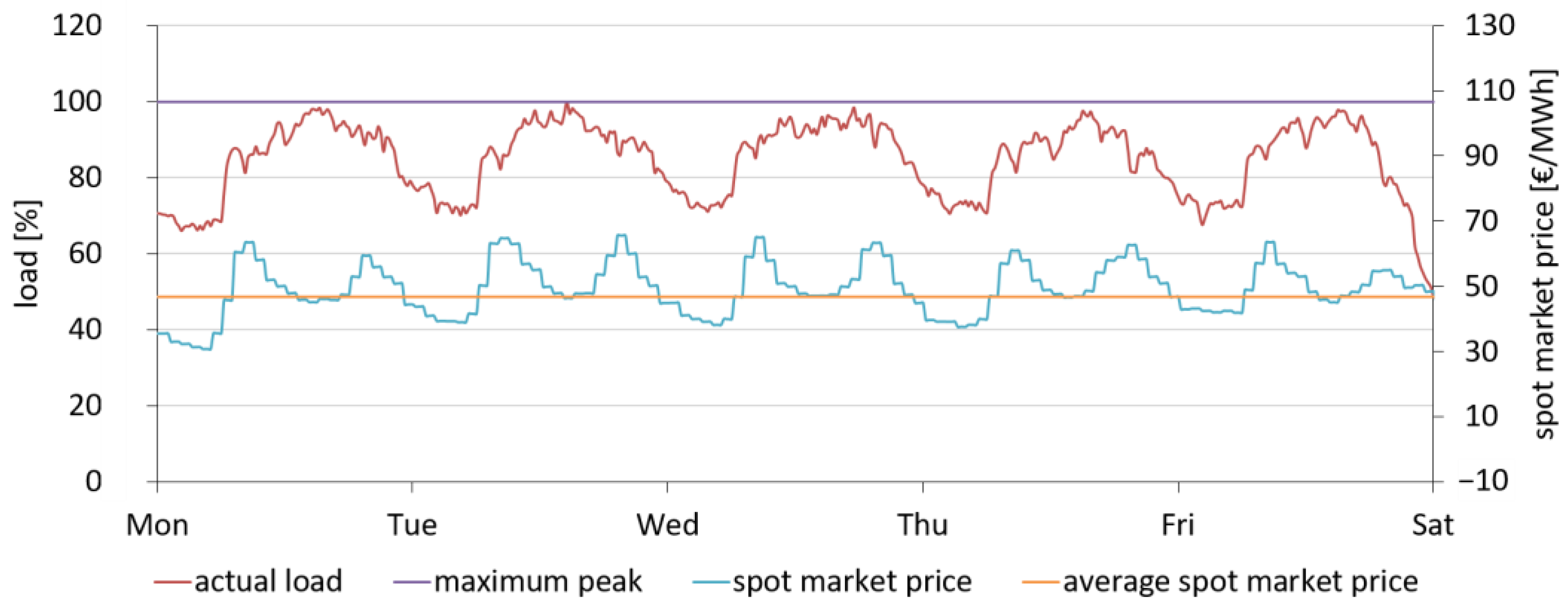
Figure 11.
Load forecast and spot market prices.
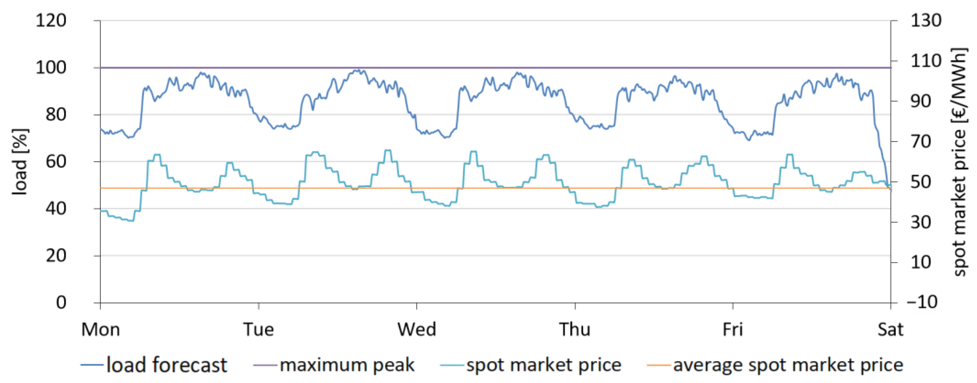
Figure 12.
Load forecast + offset and spot market prices.

Table 1.
Parameter analysis and its influence on the load (+++: high; ++: medium; +: low).
| Parameters | Thermal Load | Electrical Load |
|---|---|---|
| Geographical location | +++ | +++ |
| Season | +++ | ++ |
| Vacation | + | ++ |
| Weekday | ++ | +++ |
| Outdoor temperature | +++ | ++ |
| Public holidays | ++ | +++ |
| Production plan | ++ | +++ |
Table 2.
Peak shaving analysis.
| Peak Shaving [kW] | Actual Shave with Forecast [kW] | Actual Shave [%] |
|---|---|---|
| 500 | 455 | 91 |
| 1000 | 663 | 66 |
| 1500 | 551 | 37 |
| 2000 | 819 | 41 |
| 2500 | 178 | 7 |
| 3000 | 547 | 18 |
Table 3.
Offset analysis.
| Type of Offset | kW |
|---|---|
| maximum deviation | 3180 |
| average deviation | 1108 |
| average deviation (load > forecast) | 910 |
Table 4.
Analysis of storage sizing.
| Scenarios | Shave [kW] | Power [kW] | Capacity [kWh] |
|---|---|---|---|
| Actual load | 500 | 500 | 125 |
| Forecast | 455 | 500 | 437 |
| Forecast + offset | 500 | 3680 | 437 |
| Actual load | 1000 | 1000 | 312 |
| Forecast | 663 | 1000 | 1521 |
| Forecast + offset | 1000 | 4180 | 1521 |
| Actual load | 1500 | 1500 | 947 |
| Forecast | 551 | 1500 | 2896 |
| Forecast + offset | 1500 | 4680 | 2896 |
| Actual load | 2000 | 2000 | 2302 |
| Forecast | 819 | 2000 | 4602 |
| Forecast + offset | 2000 | 5180 | 4602 |
| Actual load | 2500 | 2500 | 3980 |
| Forecast | 178 | 2500 | 7050 |
| Forecast + offset | 2500 | 5680 | 7050 |
Table 5.
Spot market performance analysis.
| Scenario | Potential Annual Revenue [€] |
|---|---|
| Only charge at night | 201,292 |
| Charge based on forecast + Offset | 251,420 |
| Charge based on actual load | 266,656 |
Disclaimer/Publisher’s Note: The statements, opinions and data contained in all publications are solely those of the individual author(s) and contributor(s) and not of MDPI and/or the editor(s). MDPI and/or the editor(s) disclaim responsibility for any injury to people or property resulting from any ideas, methods, instructions or products referred to in the content. |
© 2023 by the authors. Licensee MDPI, Basel, Switzerland. This article is an open access article distributed under the terms and conditions of the Creative Commons Attribution (CC BY) license (https://creativecommons.org/licenses/by/4.0/).
Share and Cite
MDPI and ACS Style
Emde, A.; Märkle, L.; Kratzer, B.; Schnell, F.; Baur, L.; Sauer, A. Effects of Load Forecast Deviation on the Specification of Energy Storage Systems. Designs 2023, 7, 107. https://doi.org/10.3390/designs7050107
AMA Style
Emde A, Märkle L, Kratzer B, Schnell F, Baur L, Sauer A. Effects of Load Forecast Deviation on the Specification of Energy Storage Systems. Designs. 2023; 7(5):107. https://doi.org/10.3390/designs7050107
Chicago/Turabian StyleEmde, Alexander, Lisa Märkle, Benedikt Kratzer, Felix Schnell, Lukas Baur, and Alexander Sauer. 2023. "Effects of Load Forecast Deviation on the Specification of Energy Storage Systems" Designs 7, no. 5: 107. https://doi.org/10.3390/designs7050107