


Discharge Coefficients of Standard Spillways at High Altitudes

 , , , ,
Abstract
:1. Introduction and Objective
Previous Studies
2. Materials and Methods
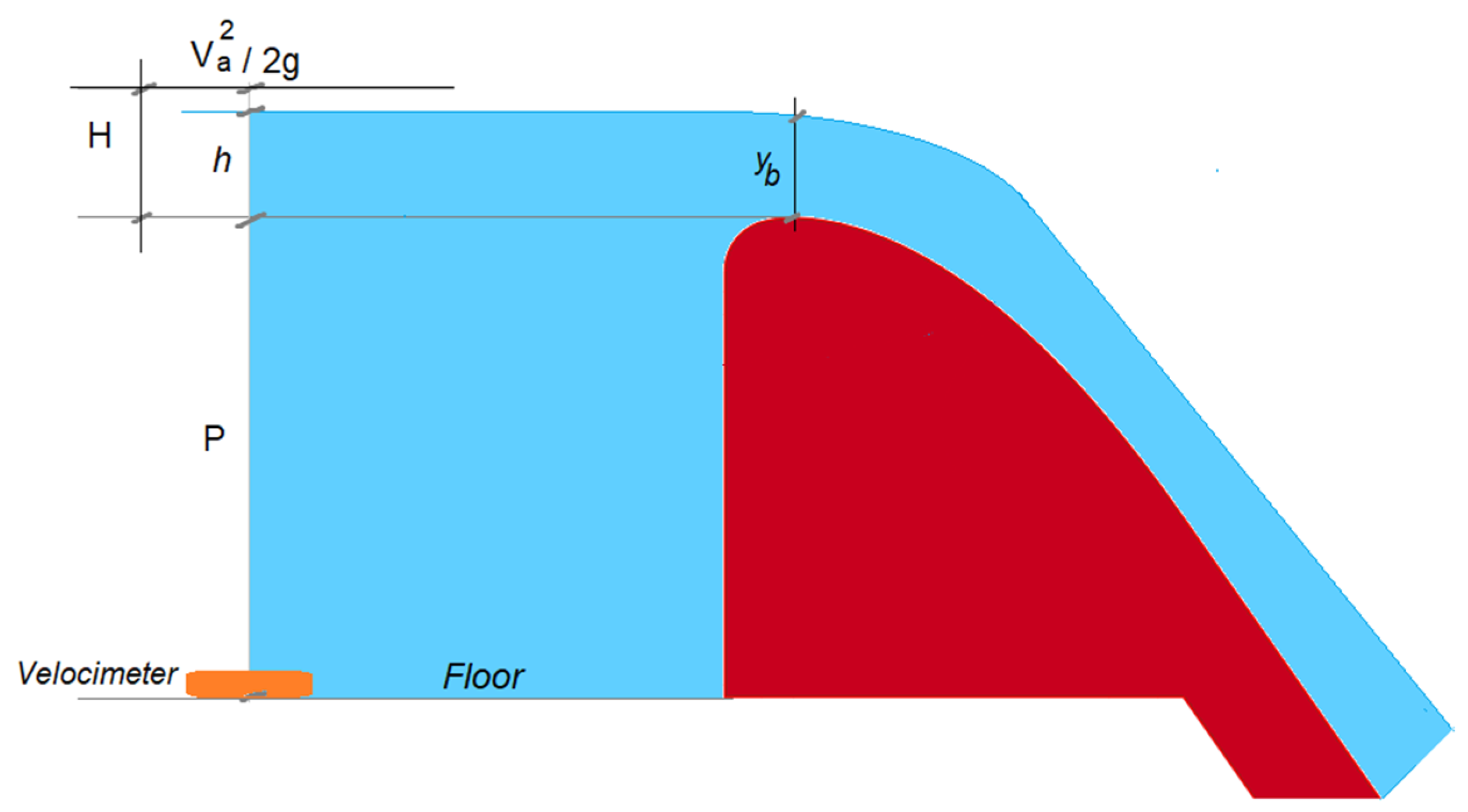
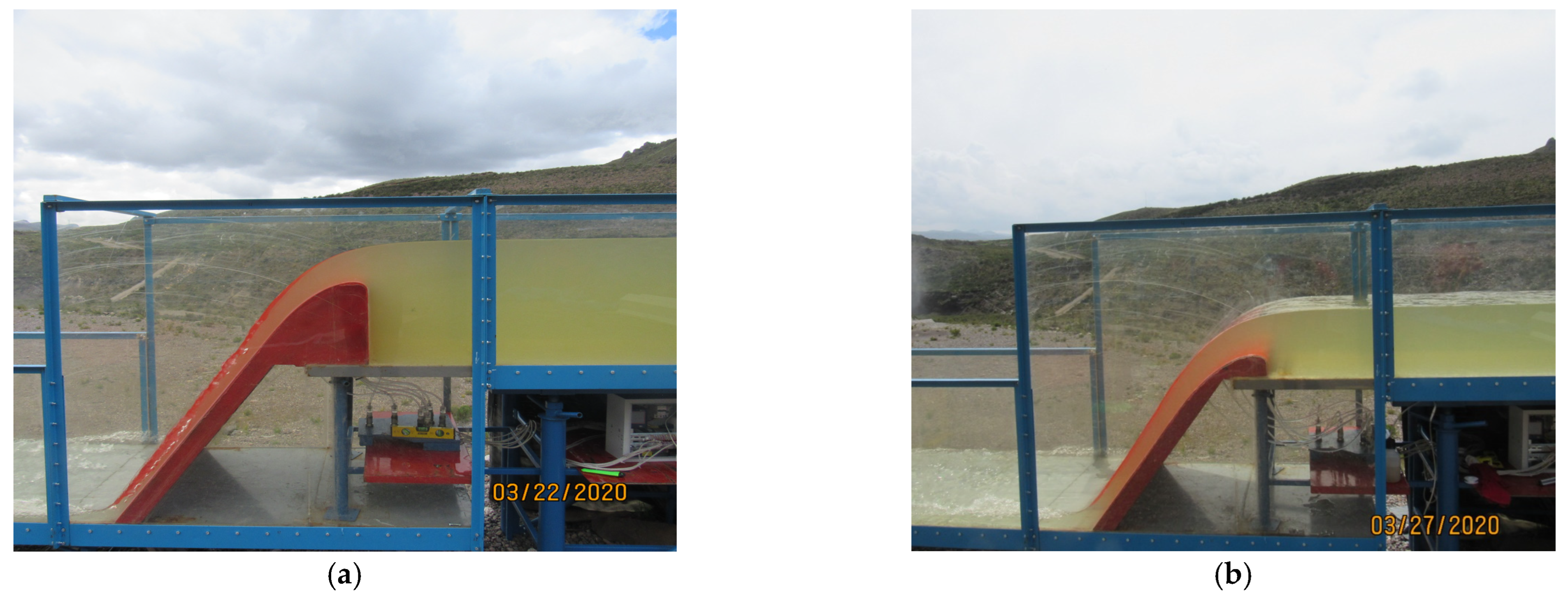
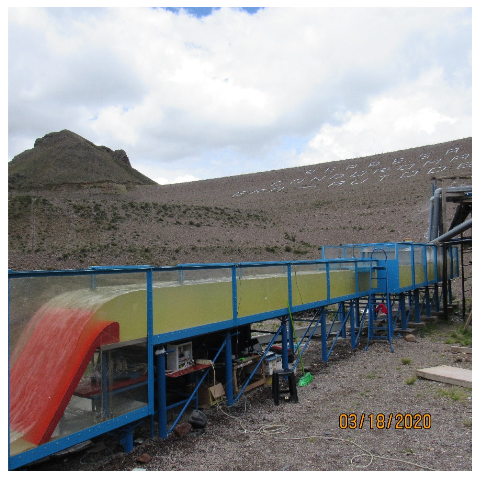
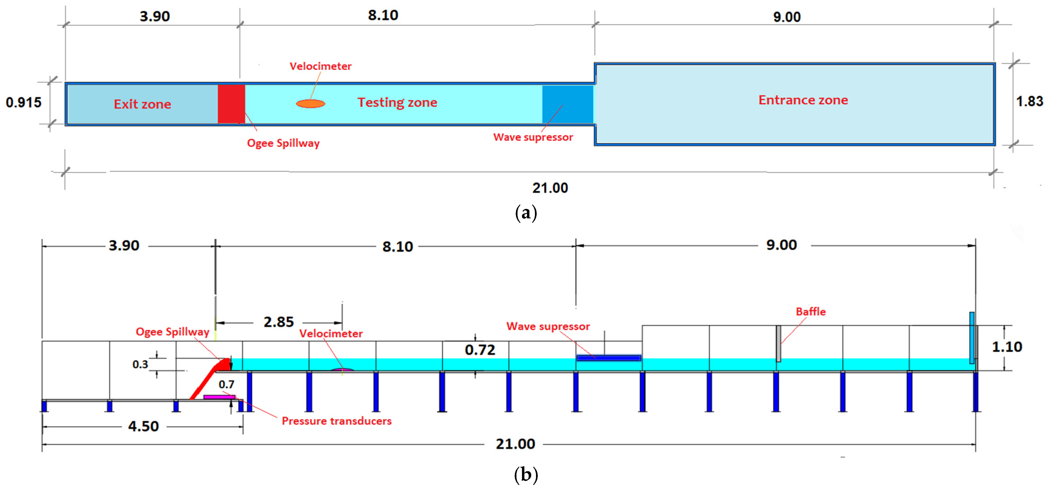
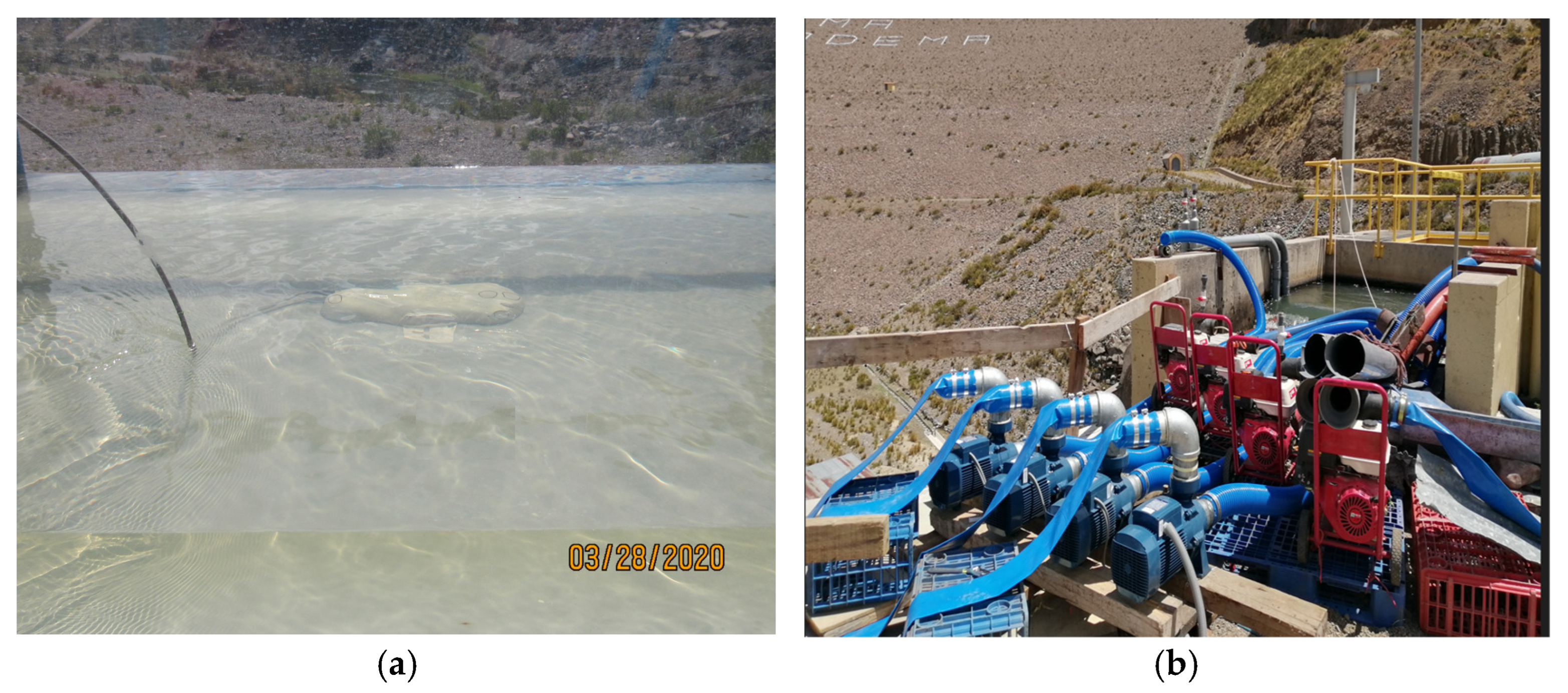
2.1. Experimental Facility
2.2. Instrumentation
2.3. Operating Conditions
2.4. Methodology
3. Results
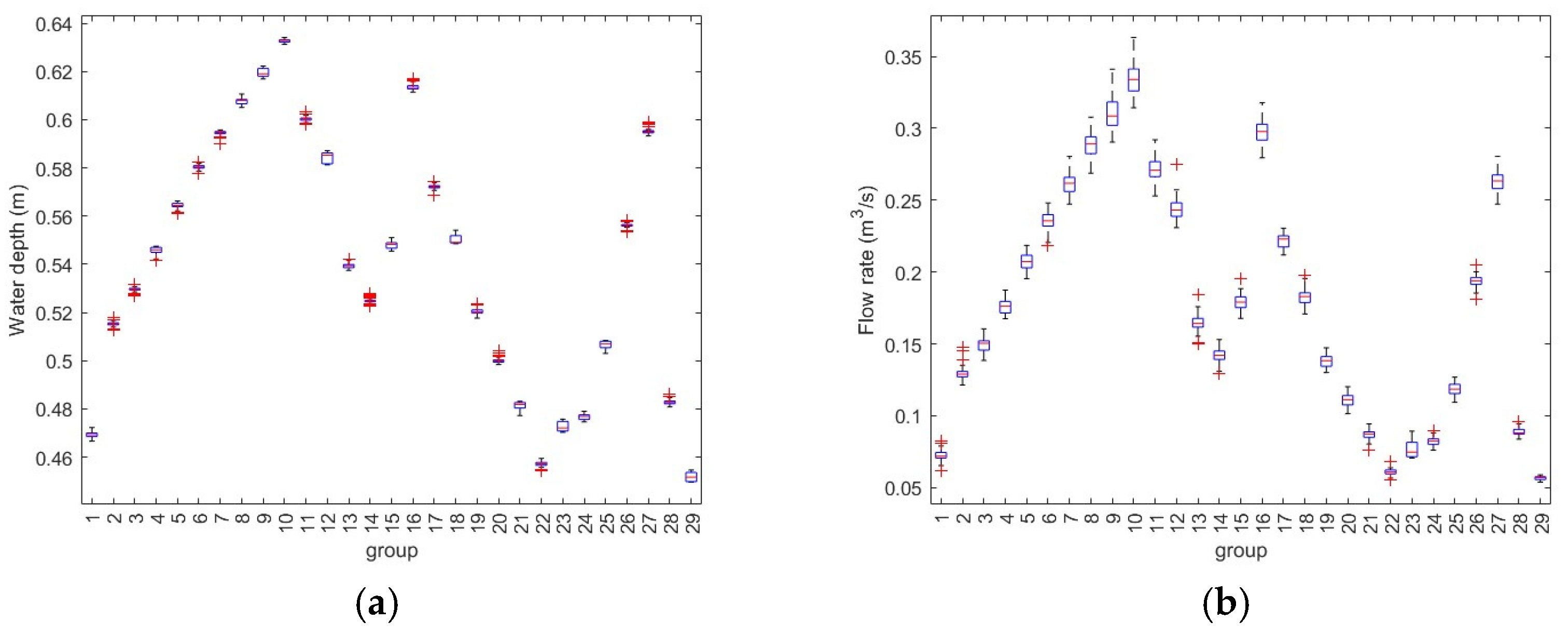
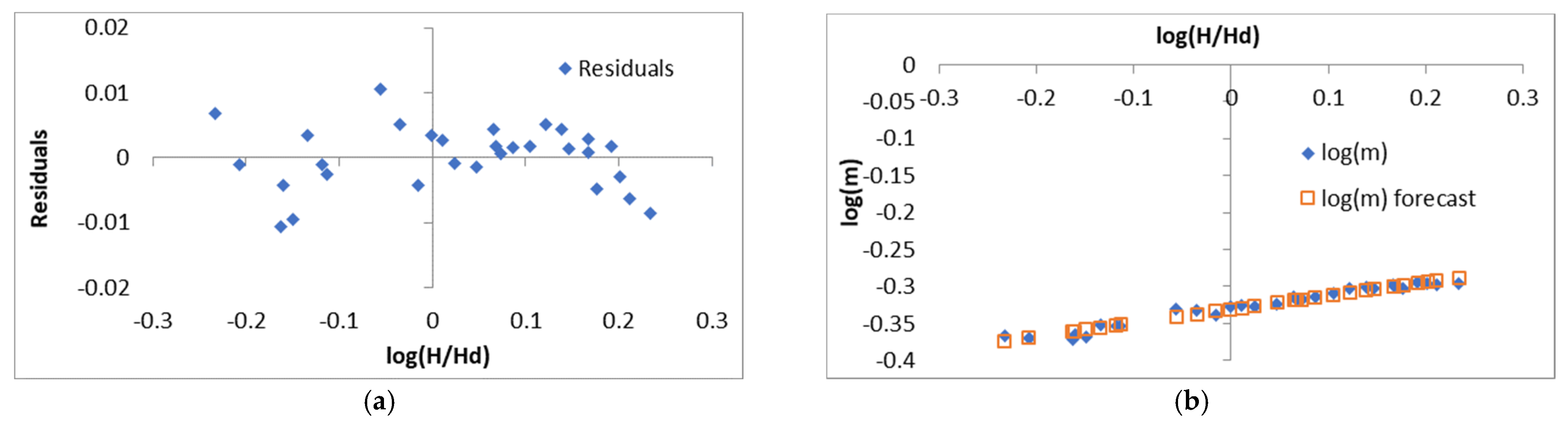
3.1. Data Processing
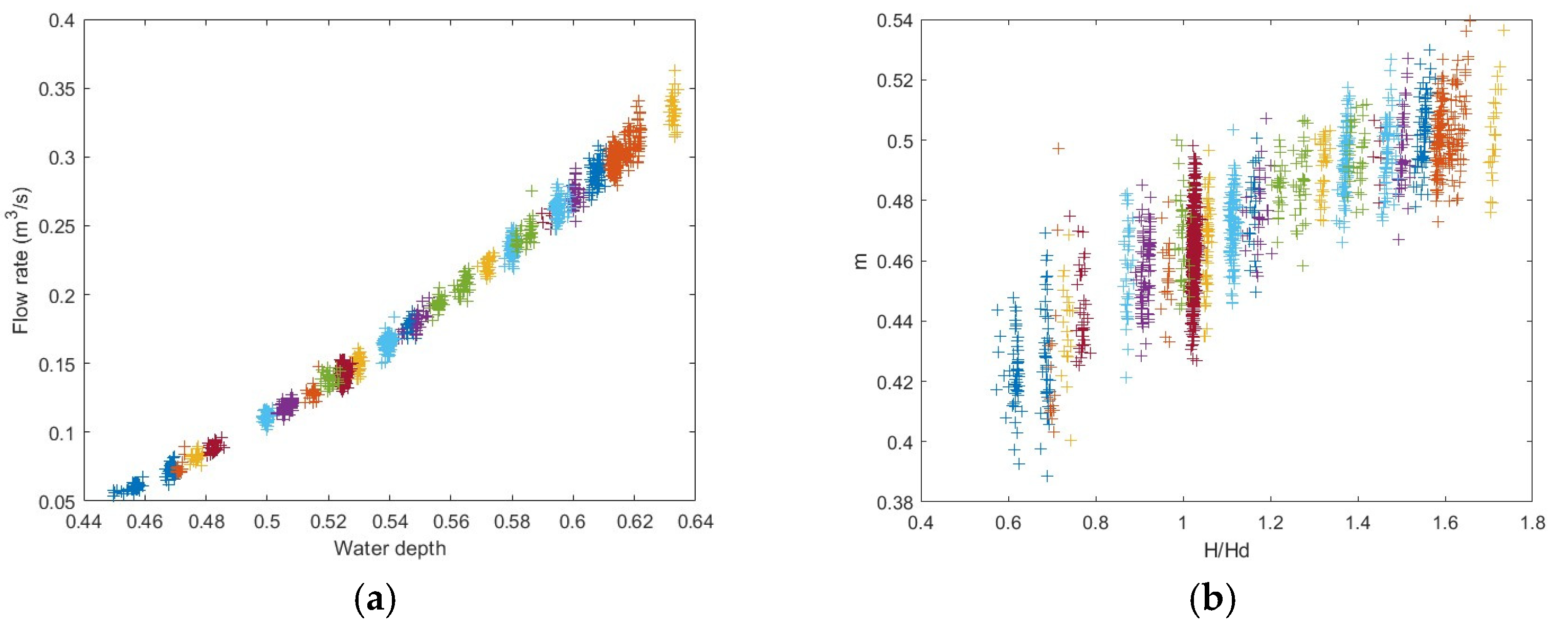

3.2. Spillway
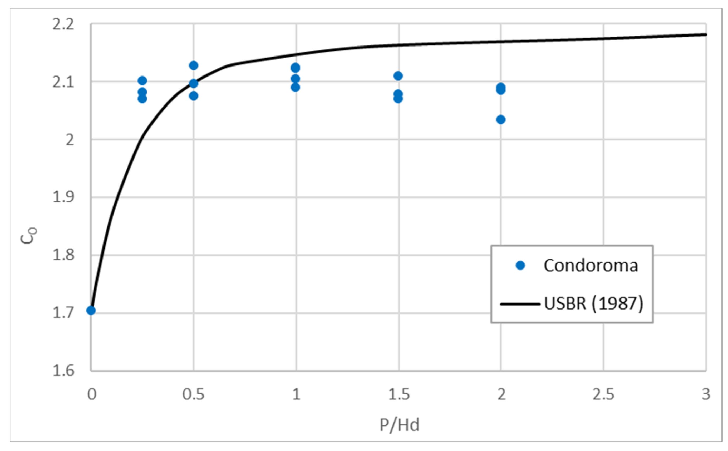
3.3. P/Hd Aggregated Analysis
4. Discussion
5. Conclusions
- -
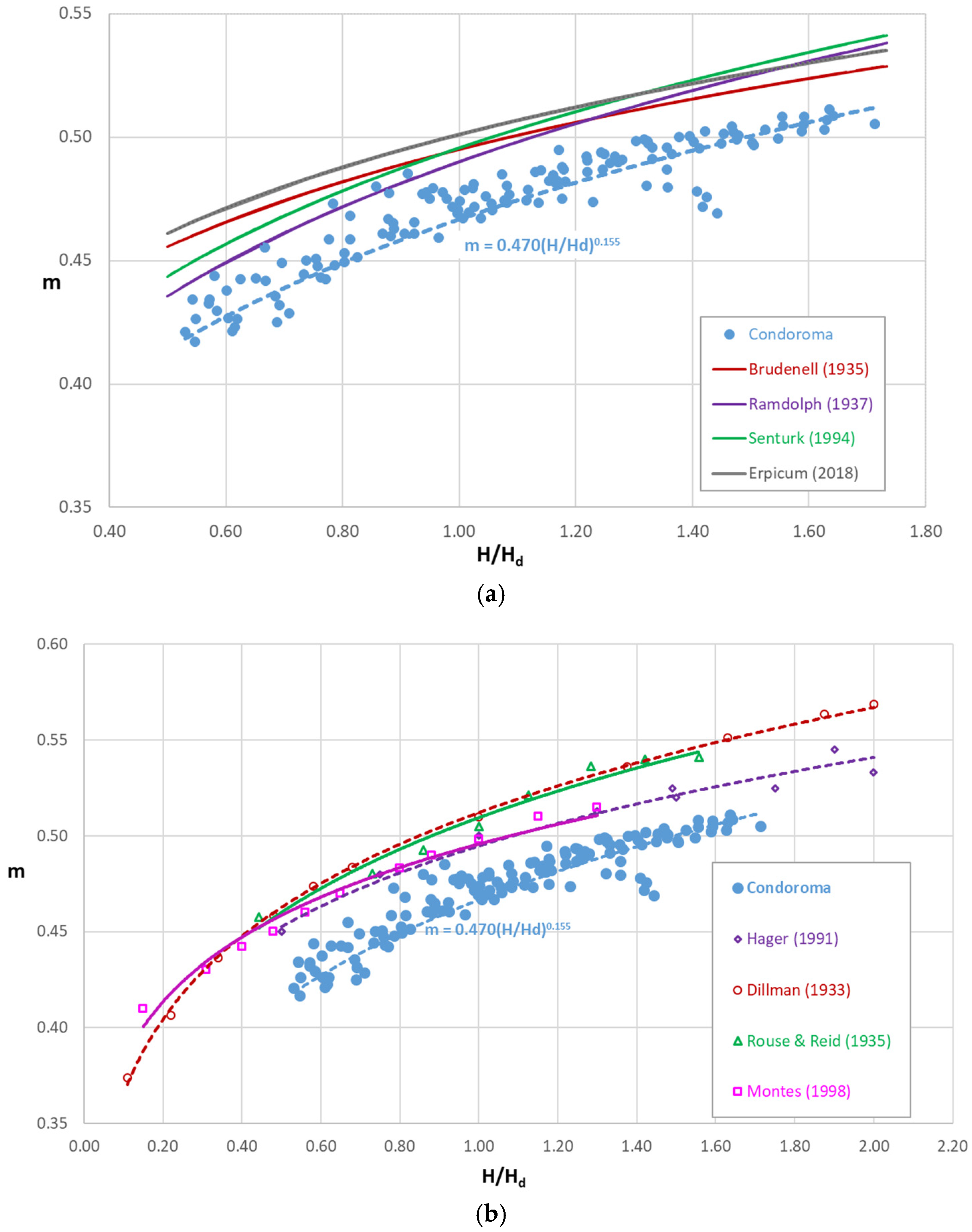
- The experimental results were compared with previous research. At altitudes above 4000 m a.s.l., the discharge coefficients show substantial differences, with consistently lower values than those obtained to date in previous works conducted at lower altitudes above sea level.
- -
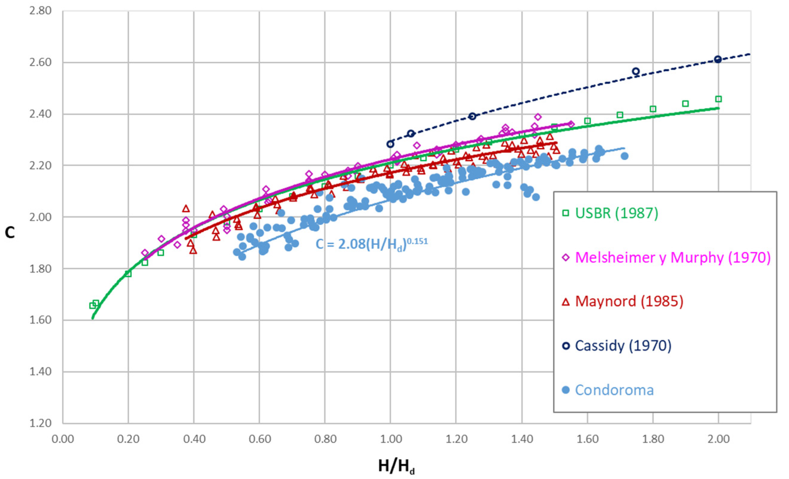
- Particularly, the discharge coefficient Co of Equation (5) when H/Hd ≈ 1 at Condoroma seems to tend towards a value slightly lower than 2.1, lower than the 2.17 proposed by USBR [4].
- -
- The P/Hd ratio influences the discharge coefficients in Condoroma, and P/Hd ≥ 1 values are recommended for the design of the spillway profile. The authors observed more stable and predictable flow behavior for higher P/Hd ratios.
- -
- Although the results obtained for P/Hd ≥ 1 at Condoroma show significantly lower values than those obtained in previous experience at much lower altitudes, it can be seen that the tests for P/Hd < 1 the discharge coefficients, although still significantly lower, are more similar to the results obtained by other authors.
- -
- The equations to determine the discharge coefficients (Equations (10) and (11)) for Condoroma could be used in areas at similar altitudes in the absence of experimental data.
Author Contributions
Funding
Data Availability Statement
Acknowledgments
Conflicts of Interest
References
- Karpenko, M.; Bogdevičius, M. Investigation of Hydrodynamic Processes in the System—“Pipeline-Fittings”. In TRANSBALTICA XI: Transportation Science and Technology: Proceedings of the International Conference TRANSBALTICA, Vilnius, Lithuania, 2–3 May 2019; Springer International Publishing: New York, NY, USA, 2020; pp. 331–340. [Google Scholar] [CrossRef]
- Han, Q.; Qu, J.; Dong, Z.; Zhang, K.; Zu, R. Air density effects on aeolian sand movement: Implications for sediment transport and sand control in regions with extreme altitudes or temperatures. J. Sedimentol. 2015, 62, 1024–1038. [Google Scholar] [CrossRef]
- Van Ingen Schenau, G.J. The influence of air friction in speed skating. J. Biomech. 1982, 15, 449–458. [Google Scholar] [CrossRef]
- United States Bureau of Reclamation. Design of Small Dams, 1960th, 1973th, 1977th ed.; Bureau of Reclamation: Denver, CO, USA, 1987. [Google Scholar]
- Naudascher, E. Hidraulica de Canales; Limusa: Mexico City, Mexico, 2002. [Google Scholar]
- Russell, G. Hydraulics, 5th ed.; Henry Holt and Company: New York, NY, USA, 1948. [Google Scholar]
- Horton, R.E. Weir Experiments, Coefficients, and Formulas; Water Supply and Irrigation Paper N°. 200; U.S. Geological Survey: Reston, VA, USA, 1907.
- Mueller, R. Development of Practical Type of Concrete Spillway Dam. Eng. Rec. 1908, 58, 461. [Google Scholar]
- Morrison, E.; Brodie, O. Mansory Dam Design; John Wiley & Sons, Inc.: Hoboken, NJ, USA, 1916. [Google Scholar]
- Creager, W. Engineering for Masonry Dams; John Wiley and Sons: New York, NY, USA, 1917; pp. 105–110. [Google Scholar]
- Nagler, F.; Davis, A. Experiments on discharge over spillway and models, Keokuk Dam. Trans. Am. Soc. Civ. Eng. 1930, 94, 777–820. [Google Scholar] [CrossRef]
- Dillmann, O. Untersuchungen an Ueberfallen; Mitteilungen des Hydraulics Institus der T.H.: Munchen, Germany, 1933; p. 7. [Google Scholar]
- Rouse, H.; Reid, L. Model research on spillway crest. Civ. Eng. 1935, 5, 10. [Google Scholar]
- Doland, J. Flow over rounded crests. Eng. News Rec. 1935, 114, 551. [Google Scholar]
- Brudenell, R. Discussion of Flow over rounded crests. Eng. News Rec. 1935, 115, 95. [Google Scholar]
- Chow, V. Open-Channel Hydraulics; McGraw-Hill Book Company: New York, NY, USA, 1959. [Google Scholar]
- Vitols, A. Vacuumless dam profiles. Wasserkr. Wasserwirtsch. 1936, 31, 207. [Google Scholar]
- Randolph, R.J. Hydraulic tests on the spillway of the Madden Dam. Trans. Am. Soc. Civ. Eng. 1937, 103, 1080–1112. [Google Scholar] [CrossRef]
- Borland, W. Flow over Crest Weirs; Civil Engineering: Fort Collins, CO, USA, 1938. [Google Scholar]
- Bradley, J. Refinements in the Design of Overfall Spillway Sections; Bureau Reclamation United States: Denver, CO, USA, 1947.
- United States Bureau of Reclamation. Studies of Crests for Overflow Dams—Bulletin 3; Bureau of Reclamation: Denver, CO, USA, 1948; pp. 1–5. [Google Scholar]
- Webster, M. Spillway Design for Pacific Northwest Projects. J. Hydraul. Div. 1959, 85, 63–85. [Google Scholar] [CrossRef]
- Cassidy, J. Spillway Discharge at other than Design Head; State Univesity of Iowa: Iowa City, IA, USA, 1964. [Google Scholar]
- Cassidy, J. Designing spillway crests for high head operation. J. Hydraul. ASCE 1970, HY3, 745–753. [Google Scholar] [CrossRef]
- Abecasis, F. Discussion of Designing spillway crests for high head operation. J. Hydraul. Div. ASCE 1970, 96, 2654–2658. [Google Scholar] [CrossRef]
- Melsheimer, E.; Murphy, T. Investigations of Various Shapes of the Upstream Quadrant of the Crest of a High Spillway; Hidraulic Laboratory Investigation: Vicksburg, MS, USA, 1970. [Google Scholar]
- Senturk, F. Hydraulics of Dams and Reservoirs; Water Resouces Publications: Littleton, CO, USA, 1994. [Google Scholar]
- Maynord, S. General Spilway Investigation; U. S. Army Corps of Engineers, Waterways Experiment Station: Vicksburg, MS, USA, 1985. [Google Scholar]
- Hager, W. Experiments on standard spillway flow. Proc. Inst. Civ. Eng. 1991, 91, 399–416. [Google Scholar]
- Saneie, M.; SheikhKazemi, J.; Azhdary Moghaddam, M. Scale Effects on the Discharge Coefficient of Ogee Spillway with an Arc in Plan and Converging Training Walls. Civ. Eng. Infrastruct. J. 2016, 49, 361–374. [Google Scholar] [CrossRef]
- Erpicum, S.; Blancher, B.; Vermeulen, J.; Peltier, Y.; Archambeau, P. Experimental study of ogee crested weir operation above the design head and influence of the upstream quadrant geometry. In Proceedings of the 7th International Symposium on Hydraulic Structures, Aachen, Germany, 15–18 May 2018. [Google Scholar]
- Alwan, H.H.; Al-Mohammed, F.M. Discharge coefficient for rectangular notch using a dimensional analysis technique. IOP Conf. Ser. Mater. Sci. Eng. 2018, 433, 012015. [Google Scholar] [CrossRef]
- Aguilera, E.; Jimenez, O. Applicability of a 3D numerical model for flow simulation of spillways. In Proceedings of the 38th IAHR World Congress, Panama City, Panama, 1–6 September 2019; p. 11. [Google Scholar]
- Roushangar, K.; Khowr, A.F.; Saniei, M. Investigating impact of converging training walls of the ogee spillways on hydraulic performance. Paddy Water Environ. J. 2020, 18, 355–366. [Google Scholar] [CrossRef]
- Hoseini, A.; Mohammadzadeh-Habili, J. Investigation of Quarter-Circular Crested Spillway Using Experiments and Convex Streamline Theory. Iran. J. Sci. Technol. Trans. Civ. Eng. 2022, 46, 1491–1501. [Google Scholar] [CrossRef]
- Alkhamis, M.T.; Sabbagh-Yazdi, S.-R.; Ranjbar-Malekshah, M. Numerical evaluation of discharge coefficient and energy dissipation of flow over a stepped morning glory spillway. J. Eng. Res. 2021, 9, 60–80. [Google Scholar] [CrossRef]
- Haktanir, T.; Khalaf, M. Discharge Coefficients for Radial-Gated Ogee Spillways by Laboratory Data and by Design of Small Dams. Tek. Dergi J. Sect. 2021, 32, 1099–10945. [Google Scholar] [CrossRef]
- Salmasi, F.; Abraham, J. Discharge coefficients for ogee spillways. Water Suply 2022, 22, 17. [Google Scholar] [CrossRef]
- Stilmant, F.; Erpicum, S.; Peltier, Y.; Archambeau, P.; Dewals, B.; Pirotton, M. Flow at an Ogee Crest Axis for a Wide Range of Head Ratios: Theoretical Model. Water 2022, 14, 2337. [Google Scholar] [CrossRef]
- Abbasi, S.; Fatemi, S.; Ghaderi, A.; Di Francesco, S. The Effect of Geometric Parameters of the Antivortex on a Triangular Labyrinth Side Weir. Water 2021, 13, 14. [Google Scholar] [CrossRef]
- Ghaderi, A.; Daneshfaraz, R.; Dasineh, M.; Di Francesco, S. Energy Dissipation and Hydraulics of Flow over Trapezoidal–Triangular Labyrinth Weirs. Water 2020, 12, 1992. [Google Scholar] [CrossRef]
- Zerihun, Y.T. Free Flow and Discharge Characteristics of Trapezoidal-Shaped Weirs. Fluids 2020, 5, 238. [Google Scholar] [CrossRef]
- Gong, J.; Deng, J.; Wei, W. Discharge Coefficient of a Round-Crested Weir. Water 2019, 11, 1206. [Google Scholar] [CrossRef]
- Jiang, L.; Diao, M.; Sun, H.; Ren, Y. Numerical Modeling of Flow Over a Rectangular Broad-Crested Weir with a Sloped Upstream Face. Water 2018, 10, 1663. [Google Scholar] [CrossRef]
- Di Bacco, M.; Scorzini, A.R. Are We Correctly Using Discharge Coefficients for Side Weirs? Insights from a Numerical Investigation. Water 2019, 11, 2585. [Google Scholar] [CrossRef]
- Yarar, A.A. Analytical and artificial neural network models to estimate the discharge coefficient for ogee spillway. E3S Web Conf. 2017, 19, 03028. [Google Scholar] [CrossRef]
- Granata, F.; Di Nunno, F.; Gargano, R.; de Marinis, G. Equivalent Discharge Coefficient of Side Weirs in Circular Channel—A Lazy Machine Learning Approach. Water 2019, 11, 12406. [Google Scholar] [CrossRef]
- Rouse, H. Discharge characteristics of the free overfall. Civ. Eng. 1936, 6, 257–260. [Google Scholar]
- Henderson, F. Open Channel Flow; The Macmillan Company: New York, NY, USA, 1966; p. 522. [Google Scholar]
- Rouse, H. The Distribution of Hydraulic Energy in Weir Flow with Relation to Spillway Design; Massachusetts Institute of Technology: Cambridge, MA, USA, 1932. [Google Scholar]
- Schoder, E.T.B. Precise weir measurements. Trans. Am. Soc. Civ. Eng. 1929, 93, 93. [Google Scholar] [CrossRef]
- Eisner, F. Overfall tests to various model scales Translation, No. 42-9, U. S. Army Corps of Engineers, Waterways Experimental Station: Vicksburg, MS, USA, 1933. [Google Scholar]
- Ghetti, A. Effects of Surface Tension on the Shape of Liquid Jets; Advanced Study Institute: Padova, Italy, 1966; pp. 424–475. [Google Scholar]
- Vischer, D.; Hager, W. Dam Hydraulics; Wiley Series: Hoboken, NJ, USA, 1998. [Google Scholar]
- Hager, W.H.; Schleiss, A.J.; Boes, R.M.; Pfister, M. Hydraulic Engineering of Dams; CRC Press: Boca Raton, FL, USA, 2021. [Google Scholar]
- Carrillo, J.; Ortega, P.; Castillo, L.; Garcia, J. Experimental Characterization of Air Entrainment in Rectangular Free Falling Jets. Water 2020, 12, 1773. [Google Scholar] [CrossRef]
- Raña, P.; Aneiros, G.; Vilar, J.M. Detection of outliers in functional time series. Environmetrics 2015, 26, 178–191. [Google Scholar] [CrossRef]
- Chapra, S.; Canale, R. Numerical Methods for Engineers, 6th ed.; CRC Press: Boca Raton, FL, USA, 2010; p. 875. [Google Scholar]
- Draper, N.; Smith, H. Applied Regression Analysis, 1st ed.; John Wiley & Sons: Hoboken, NJ, USA, 1998. [Google Scholar]
- Montes, S. Hydraulics of Open Channel Flow; ASCE Press: Reston, VA, USA, 1998. [Google Scholar]
Disclaimer/Publisher’s Note: The statements, opinions, and data contained in all publications are solely those of the individual author(s) and contributor(s) and not of MDPI and/or the editor(s). MDPI and/or the editor(s) disclaim responsibility for any injury to people or property resulting from any ideas, methods, instructions, or products referred to in the content. |


| Author | Width (m) | Hd (m) | P/Hd | Q (L/s) | Elevation m a.s.l. |
|---|---|---|---|---|---|
| Dillman [12] | - | 0.05 | - | - | 520 |
| Cassidy [24] | - | - | 2; 2.5; 3.7; 6.6 | - | 210 |
| Rouse [48] | 0.500 | - | - | 62 | 115 |
| Murphy [26] | 0.732 | 0.305 | 3.5; 7.0 | 560 | 38 |
| Maynord [28] | 0.762 | 0.249 | 0.25; 0.5; 1.0; 2.0 | 385 | 38 |
| Hager [29] | 0.500 | 0.20/0.1 | 3.5/7.0 | 375 | 495 |
| Erpicum [31] | 0.200 | 0.10/0.15 | - | 358 | 240 |
| Condoroma dam | 0.915 | 0.20/0.175 | 0.25; 0.5; 1; 1.5/2 | 415 | 4075 |
| P (m) | P/Hd | Q (L/s) | Stage (m) | Fr | yb (m) | Frb |
|---|---|---|---|---|---|---|
| (1) | (2) | (3) | (4) | (5) | (6) | (7) |
| 0.35 | 2.0 | 53–363 | 0.45–0.634 | 0.062–0.25 | 0.073–0.21 | 0.96–1.28 |
| 0.30 | 1.5 | 49–400 | 0.40–0.607 | 0.068–0.31 | 0.074–0.24 | 0.85–1.18 |
| 0.20 | 1.0 | 52–415 | 0.30–0.492 | 0.11–0.42 | 0.074–0.23 | 0.89–1.29 |
| 0.10 | 0.50 | 56–391 | 0.20–0.368 | 0.22–0.62 | 0.086–0.21 | 0.78–1.40 |
| 0.05 | 0.25 | 61–345 | 0.15–0.280 | 0.37–0.93 | 0.100–0.22 | 0.63–1.15 |
| P/Hd | Data | m0 | n | R2 |
|---|---|---|---|---|
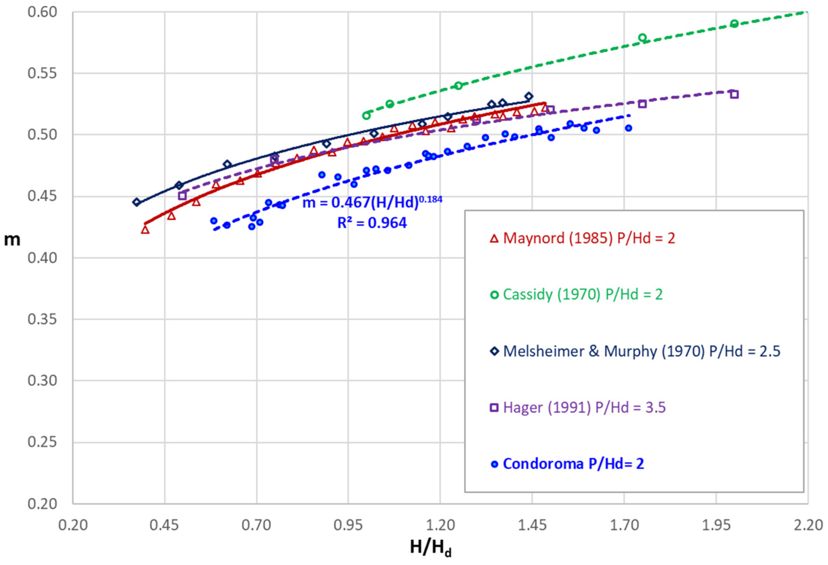
| 2.0 | Condoroma | 0.467 | 0.184 | 0.962 |
| 2.0 | Maynord [28] | 0.494 | 0.157 | 0.984 |
| 2.0 | Cassidy [24] | 0.518 | 0.186 | 0.993 |
| 2.5 | Murphy [26] | 0.503 | 0.139 | 0.974 |
| 3.5 | Hager [29] | 0.493 | 0.122 | 0.988 |
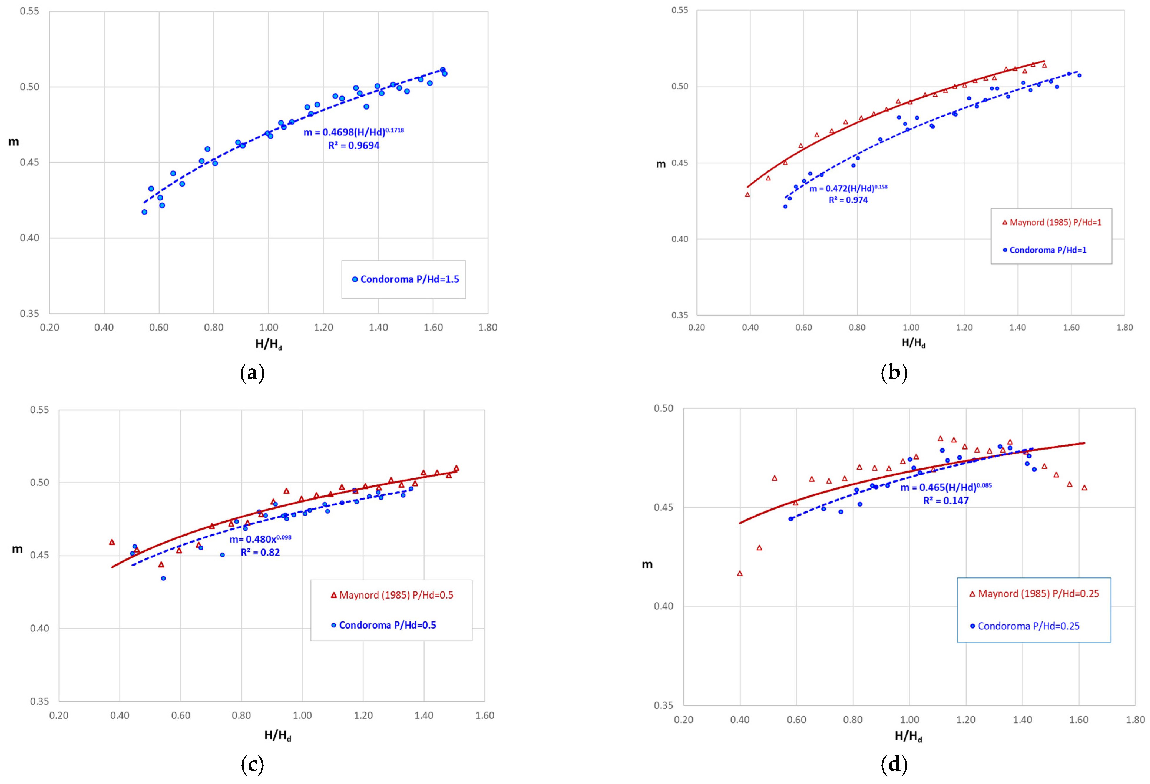
| 1.5 | Condoroma | 0.470 | 0.172 | 0.969 |
| 1 | Condoroma | 0.472 | 0.158 | 0.974 |
| 1 | Maynord [28] | 0.490 | 0.129 | 0.989 |
| 0.5 | Condoroma | 0.480 | 0.098 | 0.82 |
| 0.5 | Maynord [28] | 0.487 | 0.099 | 0.849 |
| 0.25 | Condoroma | 0.465 | 0.085 | 0.807 |
| 0.25 | Maynord [28] | 0.468 | 0.063 | 0.489 |
| Author | mo | n |
|---|---|---|
| Dillman [12] | 0.512 | 0.147 |
| Rouse [13] | 0.510 | 0.147 |
| Brudenell [15] | 0.495 | 0.120 |
| Randolph [18] | 0.490 | 0.170 |
| Cassidy [24] | 0.518 | 0.186 |
| Murphy [26] | 0.502 | 0.139 |
| Senturk [27] | 0.496 | 0.160 |
| Maynord [28] | 0.491 | 0.128 |
| Hager [29] | 0.495 | 0.129 |
| Erpicum [31] | 0.501 | 0.120 |
| Montes [60] | 0.496 | 0.113 |
| Condoroma | 0.470 | 0.151 |
Disclaimer/Publisher’s Note: The statements, opinions and data contained in all publications are solely those of the individual author(s) and contributor(s) and not of MDPI and/or the editor(s). MDPI and/or the editor(s) disclaim responsibility for any injury to people or property resulting from any ideas, methods, instructions or products referred to in the content. |
© 2024 by the authors. Licensee MDPI, Basel, Switzerland. This article is an open access article distributed under the terms and conditions of the Creative Commons Attribution (CC BY) license (https://creativecommons.org/licenses/by/4.0/).
Share and Cite
Rendón, V.; Sánchez-Juny, M.; Estrella, S.; Sanz-Ramos, M.; Rucano, P.; Huarca Pulcha, A. Discharge Coefficients of Standard Spillways at High Altitudes. Designs 2024, 8, 22. https://doi.org/10.3390/designs8020022
Rendón V, Sánchez-Juny M, Estrella S, Sanz-Ramos M, Rucano P, Huarca Pulcha A. Discharge Coefficients of Standard Spillways at High Altitudes. Designs. 2024; 8(2):22. https://doi.org/10.3390/designs8020022
Chicago/Turabian StyleRendón, Víctor, Martí Sánchez-Juny, Soledad Estrella, Marcos Sanz-Ramos, Percy Rucano, and Alan Huarca Pulcha. 2024. "Discharge Coefficients of Standard Spillways at High Altitudes" Designs 8, no. 2: 22. https://doi.org/10.3390/designs8020022