The Biomechanical Analysis of Tibial Implants Using Meshless Methods: Stress and Bone Tissue Remodeling Analysis

Abstract

Total knee arthroplasty (TKA) stands out as one of the most widely employed surgical procedures, establishing itself as the preferred method for addressing advanced osteoarthritis of the knee. However, current knee prostheses require refined design solutions. This research work focuses on a computational analysis of both the mechanical behavior of a knee joint implant and the bone remodeling process in the tibia following implantation. This research study delves into how specific design parameters, particularly the stem geometry, impact the prosthesis’s performance. Utilizing a computed tomography scan of a tibia, various TKA configurations were simulated to conduct analyses employing advanced discretization techniques, such as the finite element method (FEM) and the radial point interpolation method (RPIM). The findings reveal that the introduction of the implant leads to a marginal increase in the stress values within the tibia, accompanied by a reduction in the displacement field values. The insertion of the longest tested implant increased the maximum stress from 5.0705 MPa to 6.1584 MPa, leading to a displacement reduction from 0.016 mm to 0.0142 mm. Finally, by combining the FEM with a bone remodeling algorithm, the bone remodeling process of the tibia due to an implant insertion was simulated.

1. Introduction

Total knee arthroplasty (TKA) stands as one of the frequently conducted surgical interventions in the field of Orthopedics, offering the promise of enhancing functionality, alleviating pain, and reinstating the quality of life for patients [1]. It is estimated that in the USA, the growth in surgical requests from 2005 to 2030 will be around 673% (3.48 million) [1]. The main objective of a TKA is to reduce knee pain, based on the replacement of most of the damaged components of the joint with an implant, and the success of the surgery is estimated by the absence of pain and functional recovery of the knee in a short period [2]. TKA can encompass the surface of up to three bones: the femur, the patella, and the tibia; however, the latter is the area where most injuries leading to this surgical procedure occur [2]. In certain cases, for enhanced implant fixation and stability, a cylindrical extension known as the tibial stem is incorporated at the distal end of the tibial metal component whose primary function is to increase implant stability, particularly in challenging cases, by minimizing micromovements at the bone–implant interface, thereby mitigating the risk of aseptic loosening [3]. These tibial extensions come in various lengths and widths and can be secured through different methods, including total cementation, proximal cementation only, or a press-fit approach without the use of cement [3]. The existence and design of the tibial extension, including its size and method of fixation, can induce a phenomenon referred to as stress shielding, resulting in bone loss in the regions most affected, which may weaken the implant fixation, requiring the placement of a new prosthesis [4,5,6,7]. Stems are fundamental in most TKAs in aiding the transfer of loads from the damaged articular and metaphyseal bone to the tibial cortical limit and in distributing the increased stress of a specific joint [8]. Stems, at the cost of stress shielding, improve mechanical stability through shearing resistance, reduction in lift-off, and a decrease in micromovement [8]. In cases where the available bone reserve is inadequate to sustain the prosthesis, the incorporation of stems is generally advised [9]. When addressing substantial volume defects through bone grafting, the use of a stem becomes essential to shield the graft from excessive loads, since the knee joint bears loads several times the body weight and a failure in load transfer by the stem can subject the remaining trabecular bone to a load surpassing its maximum strength, resulting in a compromise in the fixation of the component [9]. While there is today a large consensus about the necessity of a stem for enhancing both the initial mechanical stability and the ultimate longevity of the component, the recommended lengths and diameters and fixation methods continue to be subjects of controversy [8]. It is noteworthy that it is highly unlikely that an ideal length, for example, will ever be determined, due to a huge heterogeneity in the anatomical characteristics of patients [8,10].

In cemented arthroplasty, the oldest fixation method, the cement ensures the union between the implant and the bone tissue, providing a uniform load distribution throughout the extent of the bone–implant interface [11]. However, the cement, usually composed of polymethyl methacrylate (PMMA), does not provide adhesive properties; it only fills the gaps located between the bone and the prosthesis [11]. Many studies have indicated that cemented fixation shows better short- and medium-term results, as it reduces patient pain and increases mobility and, consequently, their quality of life [11]. This method is mainly employed in cases of extensive bone damage and a significantly compromised internal cortex, particularly observed in individuals diagnosed with advanced osteoporosis [8]. However, some incidents with the use of cement have also been reported, as it degrades over time, causing the release of debris that leads to inflammation of the surrounding bone [12]. Another point to consider is the surgical intervention of revision, recurrent in younger patients, since the removal of the cement-fixed prosthesis is quite complicated, and therefore, this technique is then recommended only for patients over 65 years of age or patients with poor bone condition, in order to ensure a strong primary fixation [12,13]. The adversities and complexity related to cemented arthroplasty have encouraged the search for new fixation methodologies.

Unlike cemented arthroplasty, which results from the mechanical fixation of the cement, uncemented arthroplasty is based not only on mechanical fixation but also on the biological junction of the implant to the bone tissue [14]. This new technique aims to improve, in the long term, the success of implants in young patients, who demonstrate good bone quality. The main drawback of this approach is the pain in the lower limbs, which is a consequence of the poor fixation of the implant to the bone tissue [12].

Computational tools such as the FEM have been very useful for researchers in the field of arthroplasty. Studies using these tools focus on the implant geometry and materials as well as surgical techniques. With these studies, issues such as the minimization of stress shielding or micromotions, which can heavily hinder the success of the treatment, are dealt with. Completo et al. [15] conducted a study using the finite element method, which evaluated the distribution of loads and stability at the cement-bone interface for two fixation techniques, cemented and press-fit. The findings revealed that the load transmitted from the cemented stem to the bone was fourfold higher [15]. Quevedo González et al. [16] used a computational approach to study the effect on tibial stress of using a smaller tibial baseplate in order to prevent excessive rotation, having concluded that the consequences of this undersizing are minimal. Quevedo Gonzalez et al. [17] used a computational approach to determine that adding an anterior spike to the tibial baseplate would help to decrease the micromotions between the bone and the implant. Other approaches addressing implant geometry include the work of Liu et al. [18], who used a topology-optimization approach to improve the design of the metal plate, through a porous design, used to treat defects in the proximal tibia with TKA. Liu et al. [19] compared two techniques used in TKA, namely, the cement screw and the metal block, and concluded that the use of a metal block is more suitable for larger defects. Regarding the study of the most suitable materials, studies such as those of Bhandarkar and Dhatrak [20] and Apostolopoulos et al. [21] deal with the cushion material and tibial insert, respectively. In the first study, it is concluded that using a UHMWPE cushion leads to lower stresses in the inserts, and in the second work, an all-polyethylene TKA is compared to a metal-backed TKA and it is stated that the all-polyethylene one is cheaper and yields similar results to the metal one, with the disadvantage of requiring cement and having less flexibility. Finally, some studies concerning the arthroplasty of the ankle can also be mentioned, such as that of Jyoti and Ghosh [22] concerning the optimal resection length, which concluded that stress shielding and micromotion increase with resection depth, and thus, that this should be kept to a minimum; and the work of Jyoti et al. [23] concerning the interface of the implant, in which it is proposed that both the friction coefficient between the implant and the bone, and the implant design, along with the bone quality, heavily influence micromotion, while stress distribution is less influenced by the friction coefficient and more by the design of the implant and the quality of the bone.

The present computational approach aims at complementing experimental studies and international standards such as ISO DIS 22926 [24] and ISO/CD 5092:2023 [25]. Furthermore, this research employs meshless methods to achieve higher accuracy in obtaining solutions, thereby enhancing the quality of computational studies on implant biomechanics. Moreover, it incorporates a bone remodeling approach to assess if the implant could cause considerable bone loss as a result of stress shielding.

2. Numerical Formulation

2.1. Meshless Methods Formulation

Generally, in meshless methods the process initiates with the discretizaton of the problem’s physical domain with a nodal distribution. Although, as in other discretization techniques, regular nodal distributions allow more accurate and stable results to be achieved, in meshless methods nodes can be irregularly distributed over the problem domain. Geometry features such as cracks and holes can have a higher nodal density to anticipate the stress concentration that may occur. Usually, a very dense nodal distribution will lead to more accurate results, with the consequence of presenting a much higher computational cost [26].

Next, to integrate the integro-differential equations governing the physical phenomenon under study, it is necessary to create a background integration mesh. Commonly, background integration cells are created and then filled with integration points representing volume portions. Most meshless methods requiring integration apply the Gauss–Legendre integration scheme to the integration cells [26].

The previous stage is followed by the imposition of nodal connectivity through influence domains. Thus, each integration point searches for a certain number of nodes within its vicinity (generally, following a radial search). The nodes within its vicinity form the influence-domain of the integration point. The literature shows that the size of the influence domain significantly affects the performance of the method.

Then, using the nodes forming the corresponding influence domain, the shape functions (and their partial derivatives) of a given integration point are built, and matrix $\mathit{B}$, from Equation (18), can be established.

Taking the example of the displacement field $\mathit{u}$, the displacement at an integration point ${\mathit{x}}_I$ can be interpolated using the displacement values of the nodes within the influence domain of ${\mathit{x}}_I$,

$$\mathit{u}\left({\mathit{x}}_I\right)=\sum _{i=1}^{n_d}{\phi }_i\left({\mathit{x}}_I\right)\mathit{u}\left({\mathit{x}}_i\right)$$

(1)

where the number of nodes inside the influence domain of ${\mathit{x}}_I$ is represented as $n_d$, the displacement values of each node i belonging to the influence domain of ${\mathit{x}}_I$ is indicated as $\mathit{u}\left(x_i\right)$, and ${\phi }_i\left({\mathit{x}}_I\right)$ is the value on node i of the shape functions of ${\mathit{x}}_I$.

For each integration point ${\mathit{x}}_I$, a local stiffness matrix is established, ${\mathit{K}}_I$, Equation (22). Then, all local stiffness matrices are assembled into a global stiffness matrix, allowing the final discrete system of equations $\mathit{K}\mathit{u}=\mathit{F}$ to be obtained, which can be solved to obtain the displacement field $\mathit{u}={\mathit{K}}^{-1}\mathit{F}$.

2.1.1. Influence Domains

The RPIM uses the concept of influence domains, which is shown schematically in Figure 1. The influence domain consists of the set of nodes in the vicinity of the interest point. The nodes within the spatial vicinity of integration point ${\mathit{x}}_I$ constitute the influence domain of ${\mathit{x}}_I$. Influence domains can all have the same number of nodes or instead present different sizes and different numbers of nodes. Moreover, the shape of the influence domain can be any. In Figure 1a, the influence domains present the same size $\left(r_1=r_2\right)$, which leads to a different number of nodes in each influence domain, while in Figure 1b the number of nodes inside each influence domain is the same due to their different sizes: $\left(r_1\ne r_2\right)$.

2.1.2. Shape Functions

Consider the integration point ${\mathit{x}}_I\in {\mathbb{R}}^3$ and its influence domain: ${\mathit{X}}_I=\{{\mathit{x}}_1,{\mathit{x}}_2,\dots {\mathit{x}}_n\}\in {\mathbb{R}}^3$, with n being the total number of nodes within the influence domain of ${\mathit{x}}_I$. The shape function of ${\mathit{x}}_I$ is calculated using only the n nodes belonging to its influence domain. Thus, the variable field $\mathit{u}\left({\mathit{x}}_I\right)$ can be interpolated at ${\mathit{x}}_I$ using

$$\mathit{u}\left({\mathit{x}}_I\right)=\mathit{r}{\left({\mathit{x}}_I\right)}^{\mathrm{T}}\mathit{a}\left({\mathit{x}}_I\right)+\mathit{p}{\left({\mathit{x}}_I\right)}^{\mathrm{T}}\mathit{b}\left({\mathit{x}}_I\right)=\left\{\mathit{r}{\left({\mathit{x}}_I\right)}^{\mathrm{T}}\mathit{p}{\left({\mathit{x}}_I\right)}^{\mathrm{T}}\right\}\left\{\begin{array}{c}\mathit{a}\left({\mathit{x}}_I\right)\\ \mathit{b}\left({\mathit{x}}_I\right)\end{array}\right\}$$

(2)

where $\mathit{a}\left({\mathit{x}}_I\right)$ and $\mathit{b}\left({\mathit{x}}_I\right)$ are non-constant coefficients of the radial basis function (RBF), $\mathit{r}\left({\mathit{x}}_I\right)$, and of the polynomial basis function (PBF), $\mathit{p}\left({\mathit{x}}_I\right)$, respectively. Although the literature describes several distinct RBFs [27], generally, radial point interpolation techniques apply the multi-quadrics RBF (MQ-RBF) [28]:

$${\mathit{r}}_i\left({\mathit{x}}_I\right)={(d_{iI}^2+{\left(\gamma d_c\right)}^2)}^p$$

(3)

The parameter $d_c$ is the size coefficient, directly correlated with the numerical weight $w_I$ of the integration point ${\mathit{x}}_I$, and the parameter $d_{iI}$ is the Euclidean distance between the integration point ${\mathit{x}}_I$ and the node ${\mathit{x}}_i$ inside the influence domain of ${\mathit{x}}_I$. The parameters p and $\gamma$ are shape parameters and, according to [27], these should present values so that $\gamma d_a$ is almost null and p is almost unity, which maximizes the method’s performance.

The PBF possesses m terms (the monomials), which can be established using Pascal’s triangle.

$$\mathit{p}\left({\mathit{x}}_I\right)={\{p_1\left({\mathit{x}}_I\right)p_2\left({\mathit{x}}_I\right)\cdots p_m\left({\mathit{x}}_I\right)\}}^{\mathrm{T}}$$

(4)

In radial point interpolation formulations, the constant PBF $\mathit{p}\left(\mathit{x}\right)=\left\{1\right\}$ or the linear PBF $\mathit{p}\left(\mathit{x}\right)={\left\{1xyz\right\}}^{\mathrm{T}}$ is generally used.

The number of unknowns in the system $\mathit{R}\mathit{a}\left({\mathit{x}}_I\right)+\mathit{P}\mathit{b}\left({\mathit{x}}_I\right)={\mathit{u}}_s$ is $n+m$. Therefore, to build a system of equations it is necessary to include a new set of equations. The literature shows that it is necessary to impose ${\mathit{P}}^{\mathrm{T}}\mathit{a}\left({\mathit{x}}_I\right)=0$ to achieve a unique solution [27]. This leads to the following system of equations:

$$\left[\begin{array}{cc}\mathit{R}& \mathit{P}\\ {\mathit{P}}^{\mathrm{T}}& \mathbf{0}\end{array}\right]\left\{\begin{array}{c}\mathit{a}\left({\mathit{x}}_I\right)\\ \mathit{b}\left({\mathit{x}}_I\right)\end{array}\right\}={\mathit{M}}_T\left\{\begin{array}{c}\mathit{a}\left({\mathit{x}}_I\right)\\ \mathit{b}\left({\mathit{x}}_I\right)\end{array}\right\}=\left\{\begin{array}{c}{\mathit{u}}_s\\ \mathbf{0}\end{array}\right\}\Rightarrow \left\{\begin{array}{c}\mathit{a}\left({\mathit{x}}_I\right)\\ \mathit{b}\left({\mathit{x}}_I\right)\end{array}\right\}={\mathit{M}}_T^{-1}\left\{\begin{array}{c}{\mathit{u}}_s\\ \mathbf{0}\end{array}\right\}$$

(5)

where $\mathit{R}$ $[n\times n]$ is the radial moment matrix (Equation (6)), $\mathit{P}$ $[n\times m]$ is the polynomial moment matrix, (Equation (7)), and ${\mathit{u}}_s$ is a vector with the field function nodal parameters $[n\times 1]$.

$$\mathit{R}=\left[\begin{array}{cccc}{(d_{11}^2+{\left(\gamma d_c\right)}^2)}^p& {(d_{12}^2+{\left(\gamma d_c\right)}^2)}^p& \cdots & {(d_{1n}^2+{\left(\gamma d_c\right)}^2)}^p\\ {(d_{21}^2+{\left(\gamma d_c\right)}^2)}^p& {(d_{22}^2+{\left(\gamma d_c\right)}^2)}^p& \cdots & {(d_{2n}^2+{\left(\gamma d_c\right)}^2)}^p\\ ⋮& ⋮& \ddots & ⋮\\ {(d_{n1}^2+{\left(\gamma d_c\right)}^2)}^p& {(d_{n2}^2+{\left(\gamma d_c\right)}^2)}^p& \cdots & {(d_{nn}^2+{\left(\gamma d_c\right)}^2)}^p\end{array}\right]$$

(6)

$$\mathit{P}=\left[\begin{array}{cccc}{p}_1\left({\mathit{x}}_1\right)& p_2\left({\mathit{x}}_1\right)& \cdots & p_m\left({\mathit{x}}_1\right)\\ p_1\left({\mathit{x}}_2\right)& p_2\left({\mathit{x}}_2\right)& \cdots & p_m\left({\mathit{x}}_2\right)\\ ⋮& ⋮& \ddots & ⋮\\ p_1\left({\mathit{x}}_n\right)& p_2\left({\mathit{x}}_n\right)& \cdots & p_m\left({\mathit{x}}_n\right)\end{array}\right]$$

(7)

By back-substitution in Equation (2), it is possible to obtain

$${\mathit{u}}_h=\left\{\mathit{r}{\left({\mathit{x}}_I\right)}^{\mathrm{T}}\mathit{p}{\left({\mathit{x}}_I\right)}^{\mathrm{T}}\right\}{\mathit{M}}_T^{-1}\left\{\begin{array}{c}{\mathit{u}}_s\\ \mathbf{0}\end{array}\right\}=\left\{\mathit{\phi }{\left({\mathit{x}}_I\right)}^{\mathrm{T}}\mathit{\psi }{\left({\mathit{x}}_I\right)}^{\mathrm{T}}\right\}\left\{\begin{array}{c}{\mathit{u}}_s\\ \mathbf{0}\end{array}\right\}$$

(8)

In which $\mathit{\varphi }{\left({\mathit{x}}_I\right)}^{\mathrm{T}}$ represents the RPI shape function vector, and $\mathit{\psi }{\left({\mathit{x}}_I\right)}^{\mathrm{T}}$ is a neglectable vector, a by-product of the additional set of equations: ${\mathit{P}}^{\mathrm{T}}\mathit{a}\left({\mathit{x}}_I\right)=0$.

$$\mathit{\phi }\left({\mathit{x}}_I\right)=\left\{\begin{array}{cccc}{\phi }_1\left({\mathit{x}}_I\right)& {\phi }_2\left({\mathit{x}}_I\right)& \cdots & {\phi }_n\left({\mathit{x}}_I\right)\end{array}\right\}$$

(9)

Finally, the RPI shape functions verify the Kronecker delta property, which allows for the direct imposition of boundary conditions, as they pass through all the nodes in the influence domain:

$${\mathit{\phi }}_i\left({\mathit{x}}_j\right)={\mathit{\delta }}_{ij}\left\{\begin{array}{cc}1\hfill & (i=j)\hfill \\ 0\hfill & (i\ne j)\hfill \end{array}\right.$$

(10)

as well as satisfying the partition of unity:

$$\sum _{i=1}^n{\mathit{\phi }}_i\left({\mathit{x}}_i\right)=1$$

(11)

2.2. Weak Form and Discrete System of Equations

Assuming well-known essential boundaries and the initial and final time conditions (i.e., the compatibility conditions), the energy principle dictates that out of all possible displacement configurations satisfying such compatibility conditions, the unique final solution is the one minimizing the Lagrangian functional. The minimization of the Lagrangian functional for a solid with domain $\Omega$ and boundary $\Gamma$ can be represented as

$$\delta {\int }_{t_1}^{t_2}\left[\frac{1}{2}{\int }_{\Omega }\rho {\dot{\mathit{u}}}^{\mathrm{T}}\dot{\mathit{u}}\mathrm{d}\Omega -\frac{1}{2}{\int }_{\Omega }{\epsilon }^{\mathrm{T}}\sigma \mathrm{d}\Omega +{\int }_{\Omega }{\mathit{u}}^{\mathrm{T}}\mathit{b}\mathrm{d}\Omega +{\int }_{{\Gamma }_t}{\mathit{u}}^{\mathrm{T}}\overline{\mathit{t}}\mathrm{d}\Gamma \right]=0$$

(12)

where $\rho$ is the solid-mass density, $\dot{u}$ is the velocity, $\epsilon$ is the strain tensor, $\sigma$ is the stress tensor, u is the displacement vector, b are the body forces, and $\overline{t}$ are the traction forces applied to the boundary $\Gamma \in \Omega$. The first term of (12) refers to the kinetic energy and is, therefore, discarded in static problems. The second term is referent to the strain energy and the last two terms are referent to the work produced by the external forces. The variational operand can be moved inside the integral and the second integral in (12) is rearranged. Thus, for Equation (12) to be valid for the compatibility conditions, its integrand must be equal to zero. Such an equality results in the Galerkin weak form.

$${\int }_{\Omega }\delta {\epsilon }^{\mathrm{T}}\sigma \mathrm{d}\Omega ={\int }_{\Omega }\delta {\mathit{u}}^{\mathrm{T}}\mathit{b}\mathrm{d}\Omega +{\int }_{{\Gamma }_t}\delta {\mathit{u}}^{\mathrm{T}}\overline{\mathit{t}}\mathrm{d}\Gamma$$

(13)

where $\delta \epsilon$ is the virtual strain tensor and $\delta u$ is the virtual displacement.

The principle of virtual work states that if a solid body is in equilibrium, the virtual work produced by the inner stresses and the body applied external forces are null when the body experiments a virtual displacement.

The energy conservation principle states that if the work produced by the inner stresses is equal to the work produced by the applied external forces, then the body is in equilibrium. If the work produced by the applied external forces is calculated with a virtual displacement field and the work produced by the inner stresses is calculated using a virtual strain field resultant from the same virtual displacement field, then the principle of virtual work is obtained. Thus, knowing that stresses and strains are related through the generalized Hooke’s law equation, Equation (14),

$$\sigma =\mathit{D}\epsilon$$

(14)

and strains are linearly related to displacements, Equation (15),

$$\epsilon =\mathit{L}\mathit{u}$$

(15)

the weak form Equation (13) can be re-written in terms of displacement as follows:

$${\int }_{\Omega }\delta {\mathit{u}}^{\mathrm{T}}{\mathit{B}}^{\mathrm{T}}\mathit{D}\mathit{B}\mathit{u}\mathrm{d}\Omega ={\int }_{\Omega }\delta {\mathit{u}}^{\mathrm{T}}\mathit{H}\mathit{b}\mathrm{d}\Omega +{\int }_{\Gamma }\delta {\mathit{u}}^{\mathrm{T}}\mathit{H}\overline{\mathit{t}}\mathrm{d}\Gamma$$

(16)

Inverting the material compliance matrix $\mathit{C}$, it is possible to obtain the constitutive material matrix $\mathit{D}={\mathit{C}}^{-1}$. Assuming the Voigt notation, the material compliance matrix $\mathit{C}$ can be presented as

$$\mathit{C}=\left[\begin{array}{cccccc}{c}_1& c_3& c_3& 0& 0& 0\\ c_3& c_1& c_3& 0& 0& 0\\ c_3& c_3& c_1& 0& 0& 0\\ 0& 0& 0& c_2& 0& 0\\ 0& 0& 0& 0& c_2& 0\\ 0& 0& 0& 0& 0& c_2\end{array}\right]$$

(17)

where $c_1=1/E$ and $c_3=-\nu /E$, being that E and $\nu$ are the Young’s modulus and the Poisson ratio of the material, respectively. In Equation (16), $\mathit{B}$ is the deformation matrix:

$$\mathit{B}\left(x_I\right)=\sum _{i=1}^n\mathit{L}{\phi }_i\left({\mathit{x}}_I\right)=\left[\begin{array}{ccc}\frac{\partial {\varphi }_i}{\partial x}& 0& 0\\ 0& \frac{\partial {\varphi }_i}{\partial y}& 0\\ 0& 0& \frac{\partial {\varphi }_i}{\partial z}\\ \frac{\partial {\varphi }_i}{\partial y}& \frac{\partial {\varphi }_i}{\partial x}& 0\\ 0& \frac{\partial {\varphi }_i}{\partial y}& \frac{\partial {\varphi }_i}{\partial z}\\ \frac{\partial {\varphi }_i}{\partial z}& 0& \frac{\partial {\varphi }_i}{\partial x}\end{array}\right]$$

(18)

so that the strain and displacement relation is

$$\epsilon \left({\mathit{x}}_I\right)=\mathit{B}\left({\mathit{x}}_I\right)\mathit{u}$$

(19)

for any integration point ${\mathit{x}}_I$. $\mathit{H}$ is a diagonal matrix containing the shape functions $\phi \left({\mathit{x}}_I\right)$.

The virtual displacement can be removed from (16),

$${\int }_{\Omega }{\mathit{B}}^{\mathrm{T}}\mathit{D}\mathit{B}\mathrm{d}\Omega \mathit{u}={\int }_{\Omega }\mathit{H}\mathit{b}\mathrm{d}\Omega +{\int }_{\Gamma }\mathit{H}\overline{\mathit{t}}\mathrm{d}\Gamma$$

(20)

obtaining the discrete system of equations. Equation (20) can be written in the matrix form as

$${\mathit{K}}^e{\mathit{u}}^e={\mathit{F}}^e$$

(21)

where the elemental stiffness matrix ${\mathit{K}}^e$ is

$${\mathit{K}}^e={\int }_{\Omega }{\mathit{B}}^{\mathrm{T}}\mathit{D}\mathit{B}\mathrm{d}\Omega$$

(22)

and the force vector ${\mathit{F}}^e$ is given by

$${\mathit{F}}^e={\int }_{\Omega }\mathit{H}\mathit{b}\mathrm{d}\Omega +{\int }_{\Gamma }\mathit{H}\overline{\mathit{t}}\mathrm{d}\Gamma$$

(23)

Finally, the global system of equations is assembled from the element matrices so that the displacement field can be solved.

2.3. Bone Tissue Remodeling Algorithm

Bone remodeling is a vital process for bone health and maintenance, allowing bones to develop, repair, and renew throughout life. This process is complex and highly coordinated, involving the removal and replacement of deteriorated bone tissue through the activity of various cellular components. These components ensure mineral homeostasis and structural integrity [29]. The cellular groups that sequentially carry out the process of bone resorption and formation compose the bone remodeling unit, which has been termed the basic multicellular unit (BMU) [30]. Initially, a BMU is formed by osteoclasts responsible for bone resorption. Subsequently, the bone surface is covered by reversal cells and prepared for bone replacement. In the next step, osteoblasts release and deposit osteoid, the unmineralized bone matrix [29].

The bone remodeling cycle includes five sequential phases: activation, resorption, reversal, formation, and termination [29].

Several studies [31,32,33,34] affirm the correlation between the mechanical properties of bones and their apparent density. Additionally, various bone tissue models [35,36,37,38] in the literature delineate the evolution of trabecular architecture based on mechanical stimuli, employing diverse formulations and assumptions.

The apparent density of bone is given by

$${\rho }_{app}=\frac{w_{sample}}{V_{sample}}$$

(24)

where ${\rho }_{app}$ corresponds to the apparent density, $w_{sample}$ represents the wet mineralized mass of a given sample, and $V_{sample}$ represents the volume of the same sample. Alternatively, it is also possible to represent this property as a function of its porosity p:

$${\rho }_{app}={\rho }_0(1-p)$$

(25)

where ${\rho }_0$ corresponds to the density of compact bone, approximately 2.1 g/cm³, and porosity p is calculated from $V_{holes}/V_{sample}$, where $V_{holes}$ is the total volume of holes.

The apparent density holds significance in its connection to the mechanical attributes of bone tissue, specifically the elasticity modulus and ultimate stress. Belinha [26] employed polynomial laws to establish a relationship between the mechanical properties of bone tissue and apparent density, incorporating a transition density of 1.3 g/cm³ to differentiate between trabecular and cortical bone.

Thus, in this work the following phenomenological law was considered [26]:

$$E_{cortical}^{bone}\left[\mathrm{MPa}\right]=68,357.14{\rho }_{app}^3-276,771.43{\rho }_{app}^2+386,136.43{\rho }_{app}-177,644.29$$

(26)

$$E_{trabecular}^{bone}\left[\mathrm{MPa}\right]=805.86{\rho }_{app}^2+721.61{\rho }_{app}$$

(27)

$${\sigma }_c^{bone}\left[\mathrm{MPa}\right]=20.3508{\rho }_{app}^3+26.7984{\rho }_{app}^2$$

(28)

In Equations (26) to (28), $E_{cortical}^{bone}$ corresponds to the elastic modulus of cortical bone, $E_{trabecular}^{bone}$ corresponds to the elastic modulus of trabecular bone, and ${\sigma }_c^{bone}$ corresponds to the ultimate compressive stress.

In the bone remodeling process, there is strong evidence of the correlation between the loads (stress or strain) that the area is subject to, and the shape that the bone takes. This has led to the requirement to develop some semi-empirical laws in order to model how the bone will functionally adapt to the load case it is subject to. These laws are the basis for computational tools which aim at predicting bone adaptation under stress or strain states or changes in stiffness [26]. The model employed in this study [39,40,41,42,43] assumes that, regardless of the material law applied, the induced stress serves as an optimization tool. It aims to maximize structural integrity while minimizing mass. This perspective is analogous to viewing induced stress as an optimization tool, where the objective function is minimized, as discussed by Belinha [26].

Figure 2 summarizes the bone remodeling iterative algorithm.

The bone remodeling nonlinear equation is presented as a differential Equation (29) in which a temporal–spatial based functional, ${\rho }_{app}(\mathit{x},t)$, is minimized with respect to time, and where ${\rho }_{app}(\mathit{x},t):{\mathbb{R}}^{(d+1)}\mapsto \mathbb{R}$ is defined for the one temporal dimension and the d spatial dimensions.

$$\frac{\partial {\rho }_{app}(\mathit{x},t)}{\partial t}\cong \frac{\Delta {\rho }_{app}(\mathit{x},t)}{\Delta t}={\left({\rho }_{app}^{model}\right)}_{t_j}-{\left({\rho }_{app}^{model}\right)}_{t_{j+1}}=0$$

(29)

It is assumed that the d-dimensional domain is discretized in N nodes, $\mathit{X}=\{{\mathit{x}}_1,{\mathit{x}}_2,\dots {\mathit{x}}_N\}$ ∈ Ω, leading to $\mathit{Q}$ integration points, where $\mathit{Q}=\{{\mathit{x}}_1,{\mathit{x}}_2,\dots {\mathit{x}}_Q\}\in \Omega$, being that ${\mathit{x}}_i\in {\mathbb{R}}^d$. The temporal domain is discretized in iterative fictitious time steps $t_j\in \mathbb{R}$, where $j\in \mathbb{N}$. Within the same iterative time step $t_j$, the average apparent density of the iteration point ${\mathit{x}}_I$ is defined by ${\rho }_I=g\left({\sigma }_I\right)$:

$${\rho }_{app}^{model}=Q^{-1}\sum _{i=1}^Q{\left({\rho }_{app}\right)}_I$$

(30)

Then, $g\left({\sigma }_I\right):{\mathbb{R}}^3\mapsto \mathbb{R}$ is defined as in (31).

$$g\left({\sigma }_I\right)=max\left(\left\{{\sigma }_1^{-1}\left({\rho }_I\right){\sigma }_2^{-1}\left({\rho }_I\right){\sigma }_3^{-1}\left({\rho }_I\right)\right\}\right)$$

(31)

Here, ${\sigma }_j$ are the principal stresses obtained for integration point ${\mathit{x}}_I$ and ${\sigma }_j^{-1}\left({\rho }_I\right)$ are the inverse functions of ${\sigma }_j\left({\rho }_I\right)$, defined with the material law.

The inverse equation of stress as a function of apparent density (28) is then applied to the integration points with von Mises stress values inside the following interval, where ${\sigma }_m^{VM}=min\left({\sigma }^{VM}\right)$ and ${\sigma }_M^{VM}=max\left({\sigma }^{VM}\right)$:

$${\sigma }^{VM}\left({\mathit{x}}_I\right)\in \left[{\sigma }_m^{VM},{\sigma }_m^{VM}+\alpha ·\Delta {\sigma }^{VM}\right[\cup \left]{\sigma }_M^{VM}-\beta ·\Delta {\sigma }^{VM},{\sigma }_M^{VM}\right]$$

(32)

The parameters $\alpha$ and $\beta$ define the growth rate and the decay rate of the apparent density. The remodeling equilibrium is achieved when Equation (33) is verified, where $\alpha$, $\beta$ and ${\rho }_{app}^{control}$ depend on the analyzed problem.

$$\frac{\Delta \rho }{\Delta t}=0\wedge {\left({\rho }_{app}^{model}\right)}_{t_j}={\rho }_{app}^{control}$$

(33)

In summary, at each iteration the linear elastic analysis is run on the model. The elastic properties of the bone material are obtained from the density at each point using (26) and (27). With the obtained variable fields, the critical values for the variables are determined. The points with higher values of stress will have their density increased and the points with lower stress will have their density decreased, being that the new density value is determined through (28).

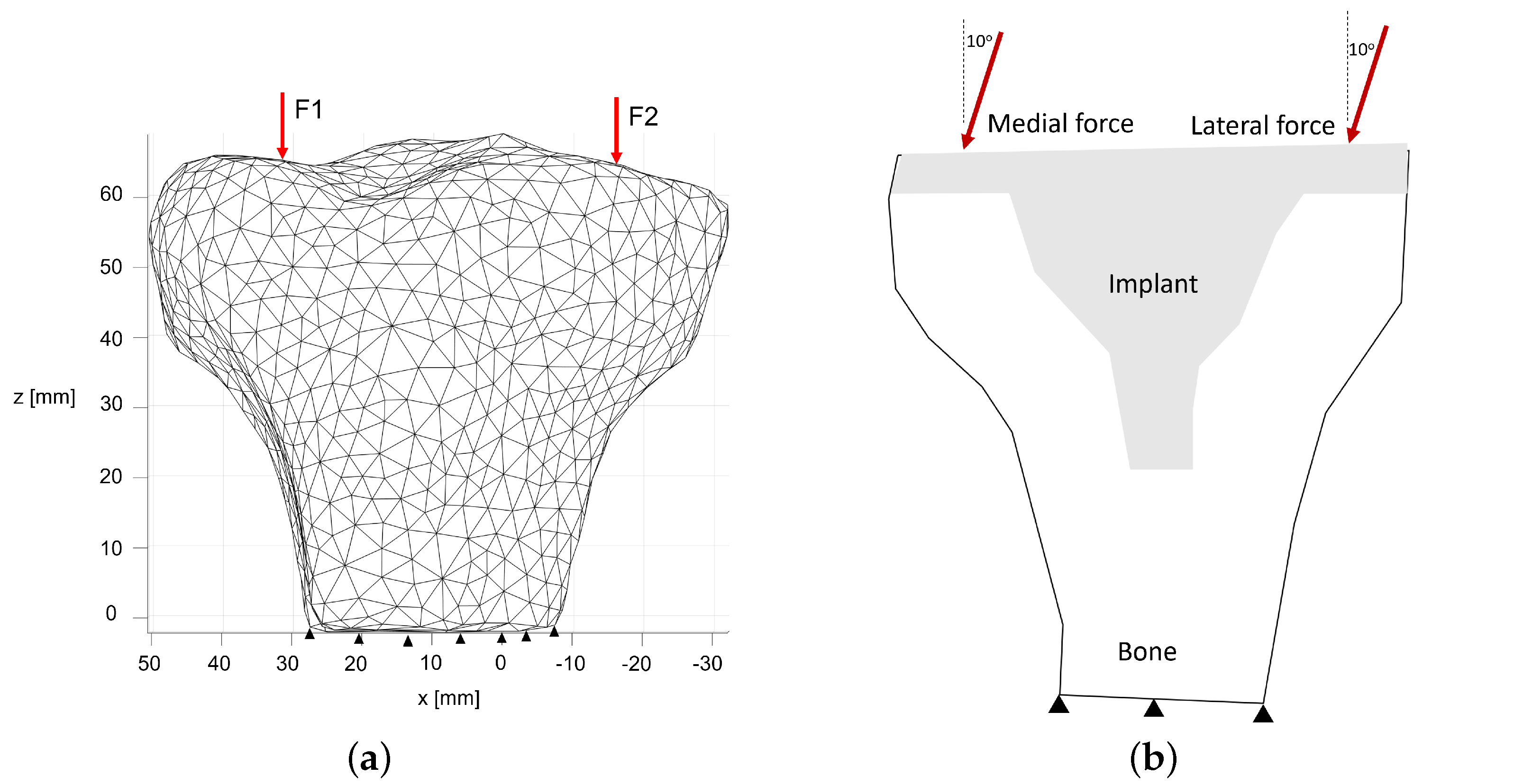
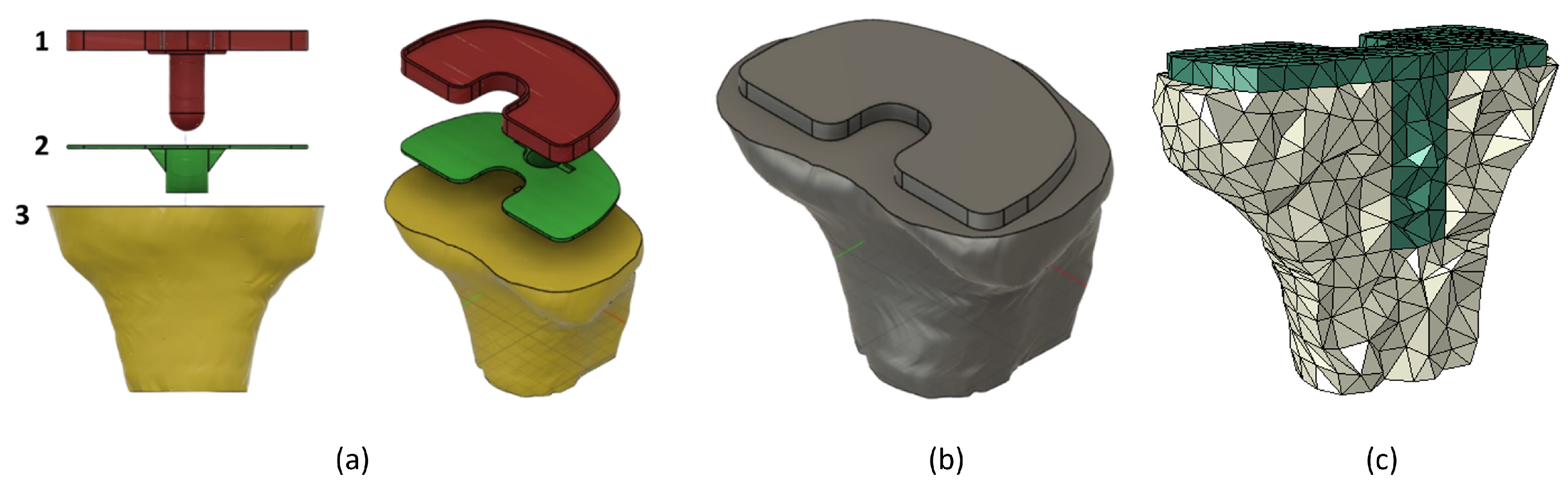
3. Tibia and Implant Numerical Models

In this section, the construction of 3D models for the numerical applications analyzed in this study is presented. Note that all the calculations were performed using an original code developed by the authors using the Matlab© (Natick, MA, USA: The MathWorks Inc.) environment. All the routines and images produced were programmed by the authors without using any toolbox of Matlab©. Nevertheless, the 3D models were created in Autodesk Fusion© (San Francisco, CA, USA: Autodesk) and the 3D discretizatons were produced with ABAQUS© (Johnston, RI, USA: Dassault Systemes Simulia Corp).

The stress and displacement analysis of the proximal tibia was run in three-dimensional models discretized into 4-node tetrahedral elements. The analysis of osteointegration to the implant was run on a two-dimensional model in order to allow for a finer mesh and, consequently, a finer trabecular arrangement. The two-dimensional model was discretized into 3-node plane-stress elements.

Table 1. Mesh information for each model.

Implant Length	Element Type	Nodes	Elements
0	4-node tetrahedral	2083	9522
12 mm	4-node tetrahedral	5273	1171
30 mm	4-node tetrahedral	6908	1487
40 mm	3-node plane stress	1901	3630
40 mm	4-node tetrahedral	6299	1360

summarizes the number of nodes and elements used for each model.

The knee joint is subjected to loads that vary significantly with the activity the individual performs. The loads applied in the model took into account another study, which analyzed the gait of an individual, where it was concluded that the average peak force was 1645 N [18]. According to the literature, the axial force is considered the primary point of evaluation of the model’s response, since it was previously determined as an indicator of injury risk. Thus, it was found that the axial load was 987 N and 658 N for the medial and lateral platforms of the tibia, respectively, since the load ratio between the medial and lateral platforms is 60%:40% [18,44]. It is important to note that the applied loads do not take into account the forces of the ligaments, muscles, and tendons. The tibia is kept in balance by the surrounding tissues and other bones of the lower limbs. The difficulty in representing this system in a finite element model leads to simplifications in terms of boundary conditions. Therefore, the nodes located at the most distal part of the model were fixed, effectively constraining any rigid-body movement.

Figure 3a shows the boundary conditions applied to the three-dimensional model without the implant. Equivalent boundary conditions were applied to the implant model as well. The loads labeled as F1 and F2 were distributed among the nodes in the vicinity of the positions indicated in Figure 3a, with moduli of 658 N and 987 N, respectively. For the remodeling analysis, the same two forces were considered. However, in order to more accurately emulate the shear loading which occurs during locomotion, these two loads were applied considering a 10º angle, as shown in Figure 3b.

Concerning the models featuring an implant, these were developed by converting the mesh model into a spline model, enabling the precise modeling of the implant’s shape. When the implant comprised three components, as depicted in Figure 4a, the model was transformed into a spline model as illustrated in Figure 4b. This simplification resulted in a unified structure with distinct material properties assigned to the bone and implant areas, as visible in Figure 4c.

Healthy cortical bone has an elastic modulus of 17 GPa; however, in this study, this property was varied (

Table 2. Mechanical properties of the implant material and cortical bone.

	Young’s Modulus [GPa]	Poisson’s Ratio
Implant—Ti-6Al-4V	110	0.34
Low-stiffness bone	5	0.33
Healthy cortical bone	17	0.33
High-stiffness bone	25	0.33

) in order to check the impact of this change on the distribution of the effective von Mises stress, as well as on the displacement field. The implant was considered to be Ti-6Al-4V.

The initial implant model shown in Figure 4a was modeled based on the the commercial implant by DePuy Synthes®.

4. Results and Discussion

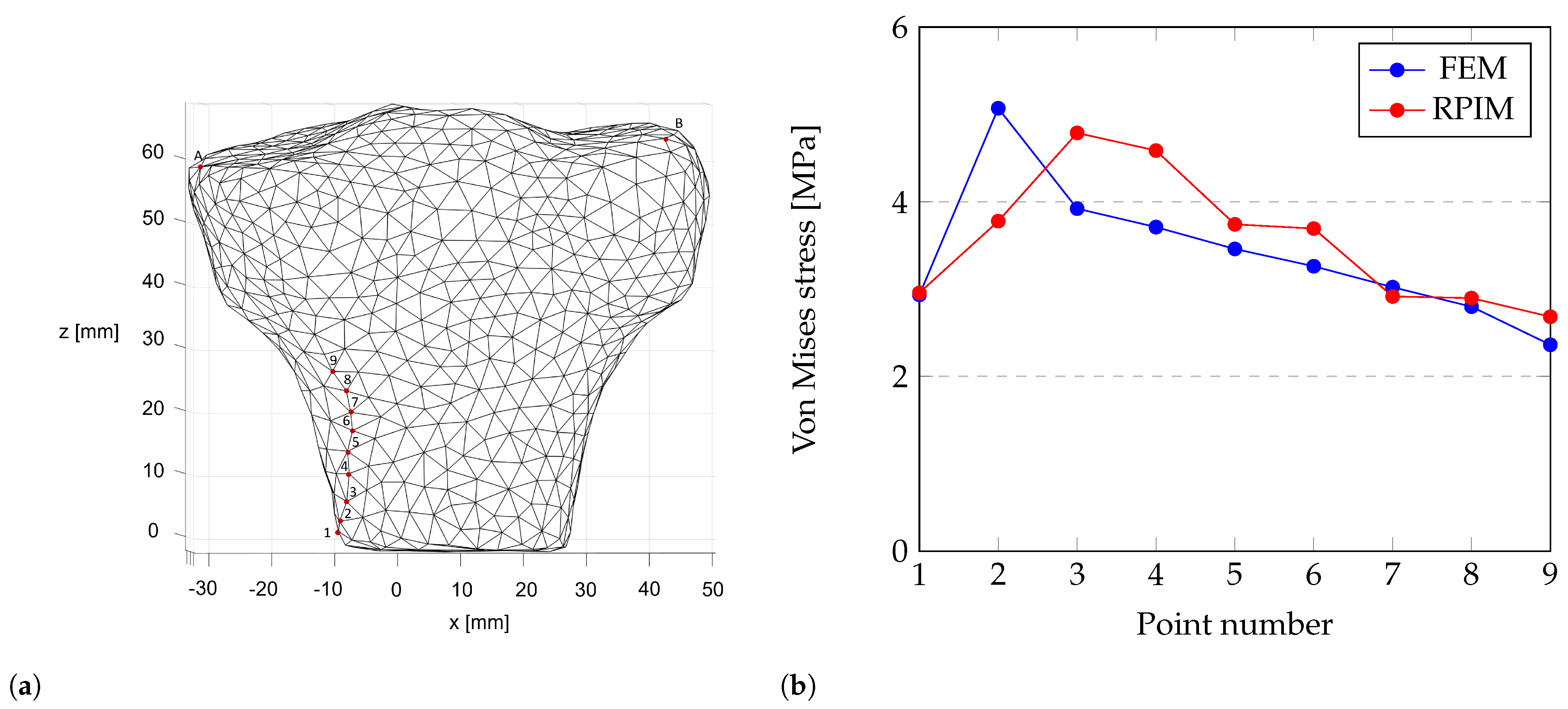
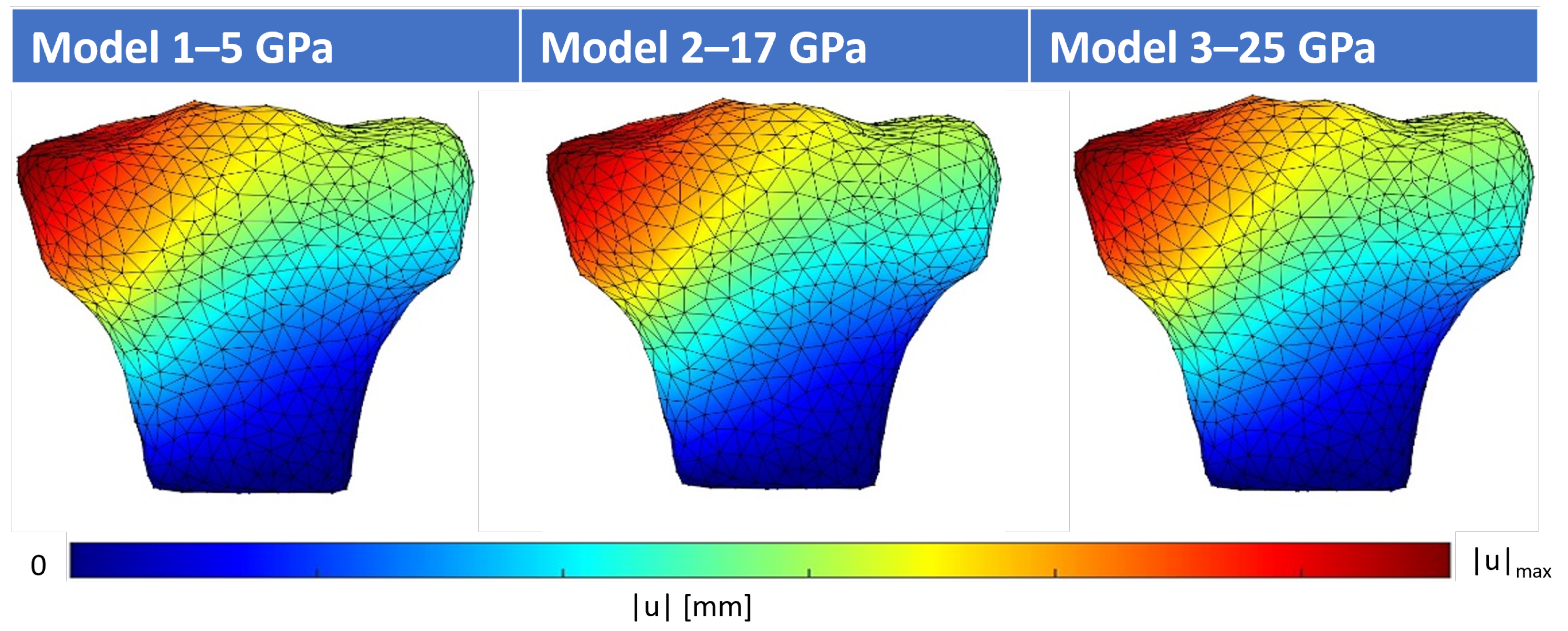
4.1. Structural Analysis of the Proximal Tibia

The Von Mises stress does not depend on the Young’s modulus of the material but it will differ between numerical methods. Thus, Figure 5 shows a set of points to evaluate the von Mises stress and the respective results.

The displacements, however, will depend on the mechanical properties. Figure 6 shows the displacement field results for the three conditions and both methods. Because the results for both methods are very similar, only one of them is shown.

Additionally, the displacement was analyzed at two points in the proximal part of the tibia, labeled in Figure 5a as point A and B. For the three materials and both methods, the displacement values are shown in

Table 3. Displacement at two points calculated with the FEM and RPIM for all tested materials.

Method	Young’s Modulus	Point	ux [mm]	uy [mm]	uz [mm]	|u| [mm]
FEM	5 GPa	A	−0.0281	−0.0158	−0.0451	0.0555
		B	−0.0241	−0.0193	−0.0035	0.031
	17 GPa	A	−0.0082	−0.0046	−0.0132	0.0163
		B	−0.007	−0.0056	−0.001	0.0091
	25 GPa	A	−0.0056	−0.0031	−0.009	0.0111
		B	−0.0048	−0.0038	−0.0007	0.0062
RPIM	5 GPa	A	−0.0286	−0.0161	−0.0471	0.0575
		B	−0.0246	−0.0203	−0.004	0.0322
	17 GPa	A	−0.0084	−0.0047	−0.0138	0.0169
		B	−0.0072	−0.0059	−0.0011	0.0094
	25 GPa	A	−0.0057	−0.0032	−0.0094	0.0115
		B	−0.0049	−0.004	−0.0008	0.0064

.

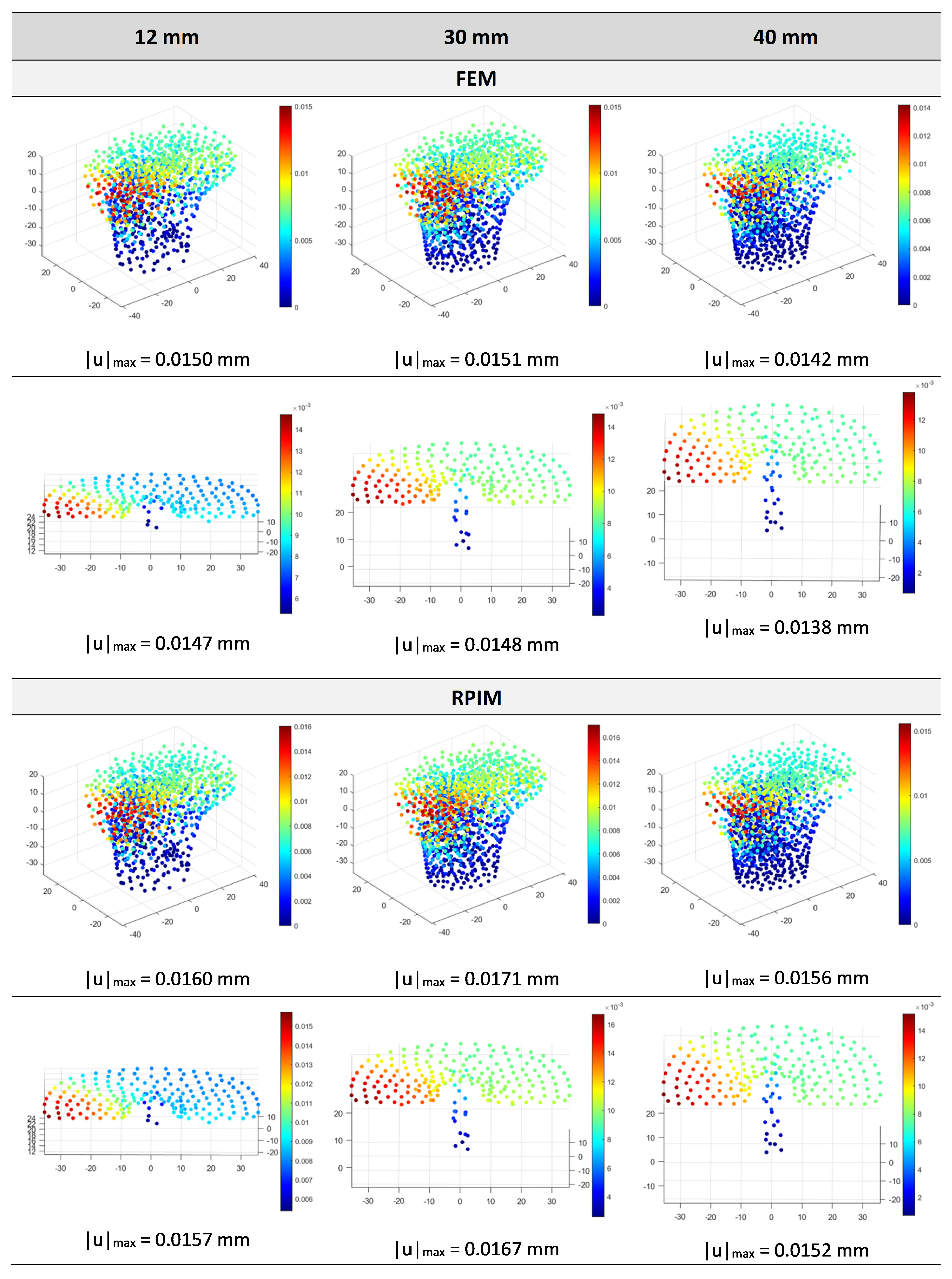
4.2. Structural Analysis of the Implant and Influence of Implant Length

The Von Mises stress fields for all the implant lengths considering healthy bone only are shown in Figure 7.

Concerning the stress analysis of the model without the implant, the FEM analysis concluded that the highest stress value occurs for point 2 while the RPIM analysis concluded that the highest stress value occurs for point 3. This phenomenon is due to the fact that the stress field is a field that has been extrapolated to the nodes, which means that the stress value is being smoothed at the nodes. By increasing the number of nodes in the mesh, this effect starts to diminish, and the maximum stress begins to approach the base of the fixture.

The maximum stress values verified after the insertion of the implant, between 5.0568 and 5.9497 MPa for the FEM and between 4.4690 and 6.1584 for the RPIM, are similar to the values verified at the unimplanted model of 5.0705 MPa for the FEM and 4.7880 MPa for the RPIM model, which indicate that stress shielding would not occur. The maximum stress values occur at similar locations for the implanted and unimplanted models.

Stress is an important measure to evaluate the occurrence of stress shielding (SS) as it indicates whether adequate loading is being applied to the bone. It can be quantified as the stress change before and after implant insertion [45] (34):

$$SS=\frac{{\sigma }_{bone}-{\sigma }_{implanted-bone}}{{\sigma }_{bone}}$$

(34)

where ${\sigma }_{bone}$ and ${\sigma }_{implantedbone}$ denote the Von Mises stress of the bone without and with the implant, respectively. Considering the maximum Von Mises stress verified at all stem lengths, the occurrence of SS can be discarded since the stress value increases after insertion.

The displacement fields for all implant lengths are shown in Figure 8.

The maximum displacement, which occurs at the medial side, is similar with and without the implant. The unimplanted model, taking into consideration the healthy bone, is 0.016 mm, while for the FEM this value ranges between 0.0142 and 0.0151 mm and 0.0156 and 0.0171 mm for the RPIM. It should be noted that the mesh model for the tibia varies with each implant length, which could account for some of the discrepancies observed between the two methods as the essential and natural boundary conditions were not being applied to the exact same nodal coordinates. Thus, excluding the RPIM analysis of the 30 mm length implant, the stress verified at the tibia would increase with implant length.

The greater the stiffness of the implant, the less load will be transferred to the bone from the deformation suffered by the stem [45]. The evaluation of displacements suffered by the implant is, therefore, an important measure of stress shielding. Since it was verified that the implant displacements are in the range of the displacements of the intact bone, similar stiffness values were achieved.

The measured displacements with the RPIM are higher than the FEM while the stress values are lower. It is expected that the results obtained through RPIM will be closer to the actual results, after conducting a convergence study (which helps to ensure that the results are more accurate), or if a denser mesh is generated, as was the case in the study developed by Marques et al. [46].

In conclusion, the tested stem sizes for an implant in the selected material are not likely to induce stress shielding. Nevertheless, this study does not consider bone heterogeneities, which alter the mechanical properties and consequently the structural response.

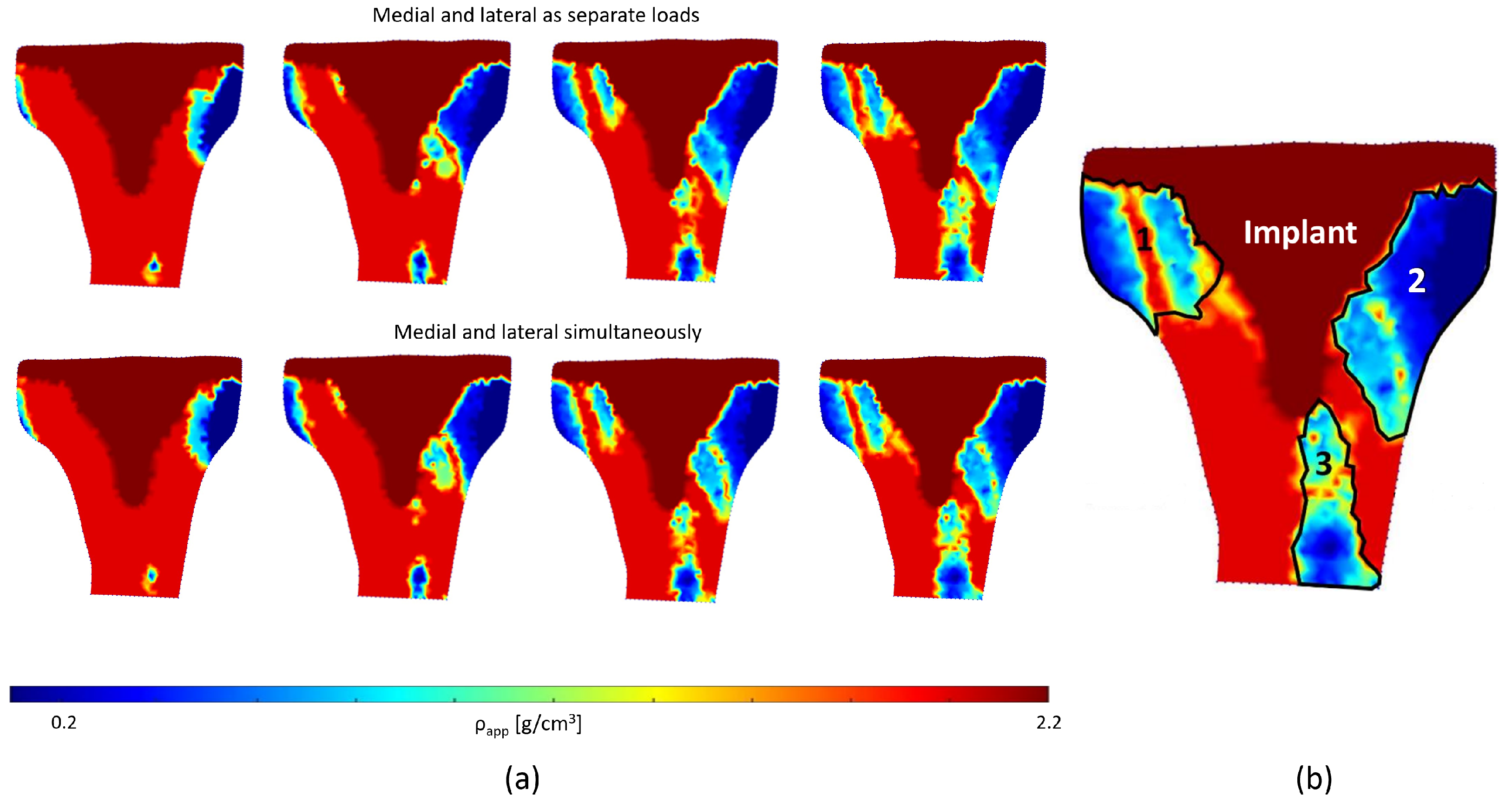
4.3. Bone Remodeling Analysis

Regarding the osteointegration evaluation, two analyses were considered. First, the medial and lateral forces were considered as two separate forces acting at two different moments, and for the second case, those forces acted simultaneously. Figure 9a shows the apparent density maps for the two tested load combinations. Only a finite element analysis was considered for this stage.

Concerning the bone remodeling analysis, there is no significant difference between the imposition of the medial and lateral loads simultaneously or as different loads. Regarding the trabecular arrangement, there are three major bone resorption areas, as indicated by the numbers in Figure 9b. Additionally the main trabecula formed by the algorithm is aligned with the load angle as expected, since the algorithm states that higher stress areas are subject to having their density increased and lower stress areas are subject to having their density decreased, leading to alignment of the density map with the stress map.

5. Conclusions

Utilizing computational approaches enhances the study of implant design and surgical techniques alongside clinical and experimental research. In summary, longer stem lengths, such as 40 mm, result in higher maximum stress in the proximal tibia but lead to lower displacements compared to shorter lengths. However, the 30 mm model stood out as an outlier in the maximum displacement due to the use of different models for testing each length. Additionally, bone remodeling analysis confirmed the expected anatomical structures, including areas of bone resorption and the diaphysis, through the observed density distribution.

References

1. Fernandes, D.A.; Poeta, L.S.; Martins, C.A.d.Q.; Lima, F.d.; Rosa Neto, F. Balance and quality of life after total knee arthroplasty. Rev. Bras. Ortop. (Engl. Ed.) 2018, 53, 747–753. [Google Scholar] [CrossRef]
2. Yueh, S.; Noori, M.; Mahadev, S.; Noori, N.B. Finite Element Analysis of Total Knee Arthroplasty. Am. J. Biomed. Sci. Res. 2021, 14, 6–15. [Google Scholar] [CrossRef]
3. Filip, A.C.; Cuculici, S.A.; Cristea, S.; Filip, V.; Negrea, A.D.; Mihai, S.; Pantu, C.M. Tibial Stem Extension versus Standard Configuration in Total Knee Arthroplasty: A Biomechanical Assessment According to Bone Properties. Medicina 2022, 58, 634. [Google Scholar] [CrossRef] [PubMed]
4. Peters, C.L.; Erickson, J.; Kloepper, R.G.; Mohr, R.A. Revision total knee arthroplasty with modular components inserted with metaphyseal cement and stems without cement. J. Arthroplast. 2005, 20, 302–308. [Google Scholar] [CrossRef]
5. Cintra, F.F.; Yepéz, A.K.; Rasga, M.G.S.; Abagge, M.; Alencar, P.G.C. Tibial Component in Revision of Total Knee Arthroplasty: Comparison Between Cemented and Hybrid Fixation. Rev. Bras. Ortop. (Engl. Ed.) 2011, 46, 585–590. [Google Scholar] [CrossRef]
6. Lonner, J.H.; Klotz, M.; Levitz, C.; Lotke, P.A. Changes in bone density after cemented total knee arthroplasty: Influence of stem design. J. Arthroplast. 2001, 16, 107–111. [Google Scholar] [CrossRef] [PubMed]
7. Shannon, B.D.; Klassen, J.F.; Rand, J.A.; Berry, D.J.; Trousdale, R.T. Revision total knee arthroplasty with cemented components and uncemented intramedullary stems. J. Arthroplast. 2003, 18, 27–32. [Google Scholar] [CrossRef] [PubMed]
8. Kang, S.G.; Park, C.H.; Song, S.J. Stem fixation in revision total knee arthroplasty: Indications, stem dimensions, and fixation methods. Knee Surg. Relat. Res. 2018, 30, 187–192. [Google Scholar] [CrossRef]
9. Crawford, D.A.; Berend, K.R.; Morris, M.J.; Adams, J.B.; Lombardi, A.V. Results of a Modular Revision System in Total Knee Arthroplasty. J. Arthroplast. 2017, 32, 2792–2798. [Google Scholar] [CrossRef]
10. Bottner, F.; Laskin, R.; Windsor, R.E.; Haas, S.B. Hybrid component fixation in revision total knee arthroplasty. Clin. Orthop. Relat. Res. 2006, 446, 127–131. [Google Scholar] [CrossRef]
11. Ni, G.X.; Lu, W.W.; Chiu, K.Y.; Fong, D.Y. Cemented or uncemented femoral component in primary total hip replacement? A review from a clinical and radiological perspective. J. Orthop. Surg. (Hong Kong) 2005, 13, 96–105. [Google Scholar] [CrossRef] [PubMed]
12. Kadir, M.R.A. Computational Biomechanics of the Hip Joint; Springer: Berlin/Heidelberg, Germany, 2013. [Google Scholar]
13. Dorr, L.D.; Wan, Z.; Gruen, T. Functional results in total hip replacement in patients 65 years and older. Clin. Orthop. Relat. Res. 1997, 336, 143–151. [Google Scholar] [CrossRef] [PubMed]
14. Kozelskaya, A.I.; Rutkowski, S.; Frueh, J.; Gogolev, A.S.; Chistyakov, S.G.; Gnedenkov, S.V.; Sinebryukhov, S.L.; Frueh, A.; Egorkin, V.S.; Choynzonov, E.L.; et al. Surface Modification of Additively Fabricated Titanium-Based Implants by Means of Bioactive Micro-Arc Oxidation Coatings for Bone Replacement. J. Funct. Biomater. 2022, 13, 285. [Google Scholar] [CrossRef] [PubMed]
15. Completo, A.; Simões, J.A.; Fonseca, F.; Oliveira, M. The influence of different tibial stem designs in load sharing and stability at the cement-bone interface in revision TKA. Knee 2008, 15, 227–232. [Google Scholar] [CrossRef] [PubMed]
16. Quevedo González, F.J.; Sculco, P.K.; Kahlenberg, C.A.; Mayman, D.J.; Lipman, J.D.; Wright, T.M.; Vigdorchik, J.M. Undersizing the Tibial Baseplate in Cementless Total Knee Arthroplasty has Only a Small Impact on Bone-Implant Interaction: A Finite Element Biomechanical Study. J. Arthroplast. 2023, 38, 757–762. [Google Scholar] [CrossRef] [PubMed]
17. Quevedo Gonzalez, F.J.; Lipman, J.D.; Sculco, P.K.; Sculco, T.P.; De Martino, I.; Wright, T.M. An Anterior Spike Decreases Bone-Implant Micromotion in Cementless Tibial Baseplates for Total Knee Arthroplasty: A Biomechanical Study. J. Arthroplast. 2023, 4–8. [Google Scholar] [CrossRef] [PubMed]
18. Liu, Y.; Chen, B.; Wang, C.; Chen, H.; Zhang, A.; Yin, W.; Wu, N.; Han, Q.; Wang, J. Design of Porous Metal Block Augmentation to Treat Tibial Bone Defects in Total Knee Arthroplasty Based on Topology Optimization. Front. Bioeng. Biotechnol. 2021, 9, 765438. [Google Scholar] [CrossRef] [PubMed]
19. Liu, Y.; Zhang, A.; Wang, C.; Yin, W.; Wu, N.; Chen, H.; Chen, B.; Han, Q.; Wang, J. Biomechanical comparison between metal block and cement-screw techniques for the treatment of tibial bone defects in total knee arthroplasty based on finite element analysis. Comput. Biol. Med. 2020, 125, 104006. [Google Scholar] [CrossRef]
20. Bhandarkar, S.; Dhatrak, P. Optimization of a knee implant with different biomaterials using finite element analysis. Mater. Today Proc. 2022, 59, 459–467. [Google Scholar] [CrossRef]
21. Apostolopoulos, V.; Tomáš, T.; Boháč, P.; Marcián, P.; Mahdal, M.; Valoušek, T.; Janíček, P.; Nachtnebl, L. Biomechanical analysis of all-polyethylene total knee arthroplasty on periprosthetic tibia using the finite element method. Comput. Methods Programs Biomed. 2022, 220, 106834. [Google Scholar] [CrossRef]
22. Mondal, S.; Ghosh, R. The role of the depth of resection of the distal tibia on biomechanical performance of the tibial component for TAR: A finite element analysis with three implant designs. Med. Eng. Phys. 2023, 119, 104034. [Google Scholar] [CrossRef]
23. Mondal, S.; Ghosh, R. Biomechanical analysis of three popular tibial designs for TAR with different implant-bone interfacial conditions and bone qualities: A finite element study. Med. Eng. Phys. 2022, 104, 103812. [Google Scholar] [CrossRef]
24. ISO 22926:2023; Implants for Surgery Specification and Verification of Synthetic Anatomical Bone Models for Testing. ISO: Geneva, Switzerland, 2023.
25. ISO/CD 5092:2023; Additive Manufacturing for Medical. ISO: Geneva, Switzerland, 2023.
26. Belinha, J. Meshless Methods in Biomechanics—Bone Tissue Remodelling Analysis; Springer: Porto, Portugal, 2014. [Google Scholar]
27. Belinha, J. Meshless Methods in Biomechanics: Bone Tissue Remodelling Analysis; Lecture Notes in Computational Vision and Biomechanics; Springer International Publishing: Berlin/Heidelberg, Germany, 2014. [Google Scholar]
28. Hardy, R.L. Theory and applications of the multiquadric-biharmonic method 20 years of discovery 1968–1988. Comput. Math. Appl. 1990, 19, 163–208. [Google Scholar] [CrossRef]
29. Raggatt, L.J.; Partridge, N.C. Cellular and molecular mechanisms of bone remodeling. J. Biol. Chem. 2010, 285, 25103–25108. [Google Scholar] [CrossRef] [PubMed]
30. Sabet, F.A.; Najafi, A.R.; Hamed, E.; Jasiuk, I. Modelling of bone fracture and strength at different length scales: A review. Interface Focus 2016, 6, 20–30. [Google Scholar] [CrossRef] [PubMed]
31. Carter, D.R.; Hayes, W.C. The compressive behavior of bone as a two-phase porous structure. J. Bone Jt. Surgery. Am. Vol. 1977, 59, 954–962. [Google Scholar] [CrossRef]
32. Goldstein, S.A. The mechanical properties of trabecular bone: Dependence on anatomic location and function. J. Biomech. 1987, 20, 1055–1061. [Google Scholar] [CrossRef]
33. Rice, J.C.; Cowin, S.C.; Bowman, J.A. On the dependence of the elasticity and strength of cancellous bone on apparent density. J. Biomech. 1988, 21, 155–168. [Google Scholar] [CrossRef]
34. Martin, R.B. Determinants of the mechanical properties of bones. J. Biomech. 1991, 24, 79–88. [Google Scholar] [CrossRef]
35. Pauwels, F. Gesammelte Abhandlungen zur Funktionellen Anatomie des Bewegungsapparates; Springer: Berlin/Heidelberg, Germany, 2013. [Google Scholar]
36. Cowin, S.C.; Hegedus, D.H. Bone remodeling I: Theory of adaptive elasticity. J. Elast. 1976, 6, 313–326. [Google Scholar] [CrossRef]
37. Cowin, S.C.; Sadegh, A.M.; Luo, G.M. An Evolutionary Wolff’s Law for Trabecular Architecture. J. Biomech. Eng. 1992, 114, 129–136. [Google Scholar] [CrossRef] [PubMed]
38. Rodrigues, H.; Jacobs, C.; Guedes, J.M.; Bendsøe, M.P. Global and local material optimization models applied to anisotropic bone adaptation. In Proceedings of the IUTAM Symposium on Synthesis in Bio Solid Mechanics, Copenhagen, Denmark, 24–27 May 1998; Springer: Berlin/Heidelberg, Germany, 1999; pp. 209–220. [Google Scholar]
39. Carter, D.R.; Fyhrie, D.P.; Whalen, R.T. Trabecular bone density and loading history: Regulation of connective tissue biology by mechanical energy. J. Biomech. 1987, 20, 785–794. [Google Scholar] [CrossRef] [PubMed]
40. Whalen, R.T.; Carter, D.R.; Steele, C.R. Influence of physical activity on the regulation of bone density. J. Biomech. 1988, 21, 825–837. [Google Scholar] [CrossRef]
41. Carter, D.R.; Orr, T.E.; Fyhrie, D.P. Relationships between loading history and femoral cancellous bone architecture. J. Biomech. 1989, 22, 231–244. [Google Scholar] [CrossRef] [PubMed]
42. Belinha, J.; Natal Jorge, R.M.; Dinis, L.M. Bone tissue remodelling analysis considering a radial point interpolator meshless method. Eng. Anal. Bound. Elem. 2012, 36, 1660–1670. [Google Scholar] [CrossRef]
43. Belinha, J.; Jorge, R.M.N.; Dinis, L.M.J.S. A meshless microscale bone tissue trabecular remodelling analysis considering a new anisotropic bone tissue material law. Comput. Methods Biomech. Biomed. Eng. 2013, 16, 1170–1184. [Google Scholar] [CrossRef]
44. Taddei, F.; Pani, M.; Zovatto, L.; Tonti, E.; Viceconti, M. A new meshless approach for subject-specific strain prediction in long bones: Evaluation of accuracy. Clin. Biomech. 2008, 23, 1192–1199. [Google Scholar] [CrossRef] [PubMed]
45. Liu, B.; Wang, H.; Zhang, N.; Zhang, M.; Cheng, C.K. Femoral Stems With Porous Lattice Structures: A Review. Front. Bioeng. Biotechnol. 2021, 9, 772539. [Google Scholar] [CrossRef]
46. Marques, M.; Belinha, J.; Dinis, L.M.J.S.; Natal Jorge, R. A brain impact stress analysis using advanced discretization meshless techniques. Proc. Inst. Mech. Eng. Part H J. Eng. Med. 2018, 232, 257–270. [Google Scholar] [CrossRef]
Figure 1. Influence domains: (a) fixed size; (b) variable size.
Designs 08 00028 g001
Figure 2. Flowchart for the bone remodeling algorithm.
Designs 08 00028 g002
Figure 3. Schematic representation of the essential and natural boundary conditions applied to (a) the three-dimensional model and (b) the two-dimensional implant model.
Designs 08 00028 g003
Figure 4. Implant model. (a) 1—tibial plate, 2—cement, 3—tibia; (b) simplified assembled model; (c) simplified model representation showing the implant and surrounding bone.
Designs 08 00028 g004
Figure 5. Von Mises stress results: (a) selected points in the model (A and B are two representative points of load application and, therefore, are used to evaluate the displacement and points 1 to 9 are the points selected to evaluate stress since each point is further from the fixed ending); (b) von Mises stress at each point calculated with the FEM and the RPIM.
Designs 08 00028 g005
Figure 6. Displacement field for each material, where the maximum displacements | u | m a x are 0.050, 0.016, and 0.010 for model 1, model 2, and model 3, respectively.
Designs 08 00028 g006
Figure 7. Von Mises stress field at the nodes for the tested implants.
Designs 08 00028 g007
Figure 8. Displacement field at the nodes for the tested implants.
Designs 08 00028 g008
Figure 9. (a) Evaluation of osteointegration using the FEM along the iterations; (b) indication of the main resorption (indicated by numbers 1 to 3) and growth areas after implant insertion.
Designs 08 00028 g009