
Structural Health Monitoring-Based Bridge Lifecycle Extension: Survival Analysis and Monte Carlo-Based Quantification of Value of Information

Abstract
:1. Introduction
2. Materials and Methods
2.1. Value of SHM Information
- Draw realizations of the degradation process from the distribution of RUL.
- Compute PVSHM for this realization using the formula presented above. The computed value represents a single simulated sample from the distribution of the SHM system’s present value.
- Repeat the process for N times to obtain N samples from the distribution of the VoI.
2.2. Lifecycle Extension: VoI Quantification
2.2.1. Dataset Used for Deterioration Modeling
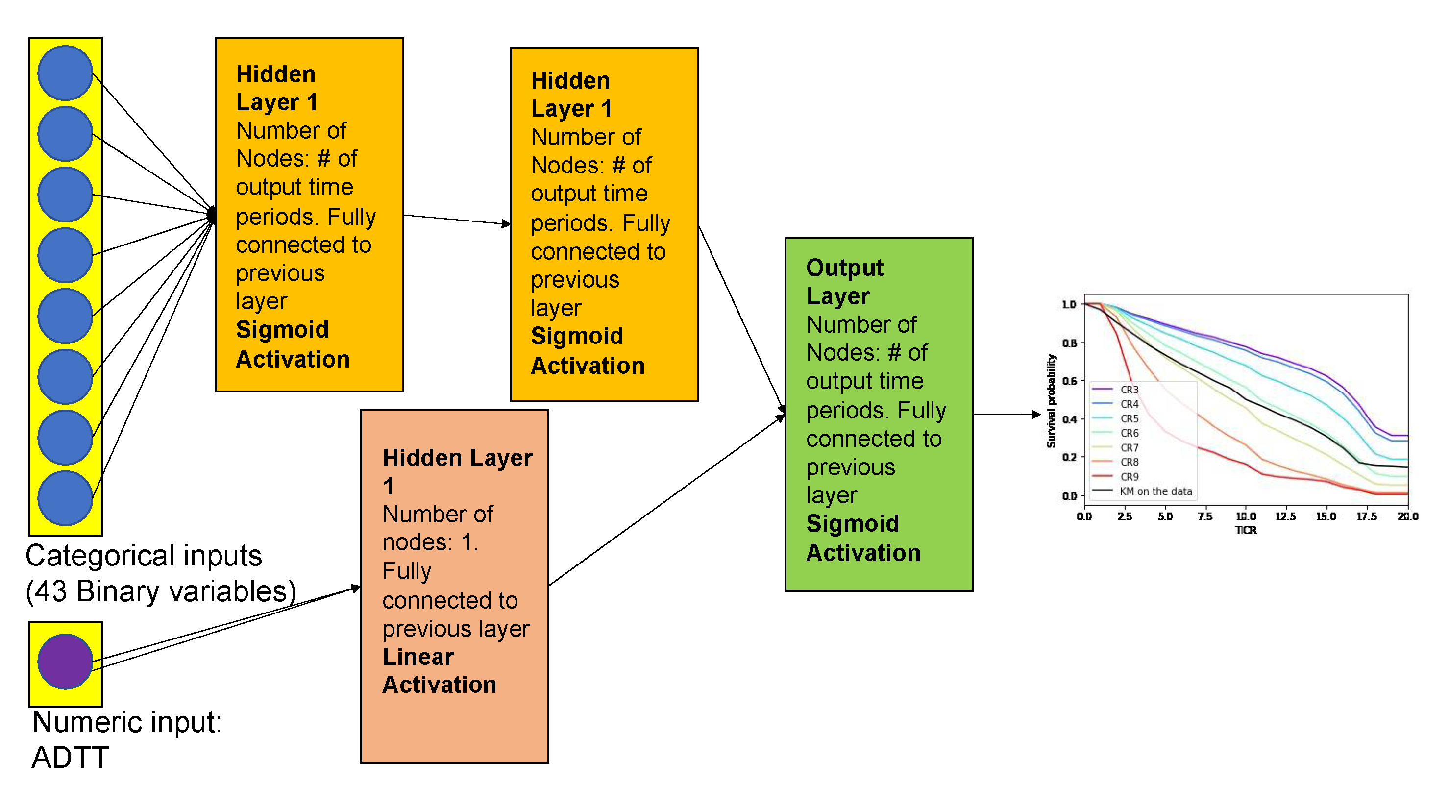
2.2.2. Computational Approach: Survival Analysis
2.2.3. Computational Approach: Monte Carlo Simulation
3. Results
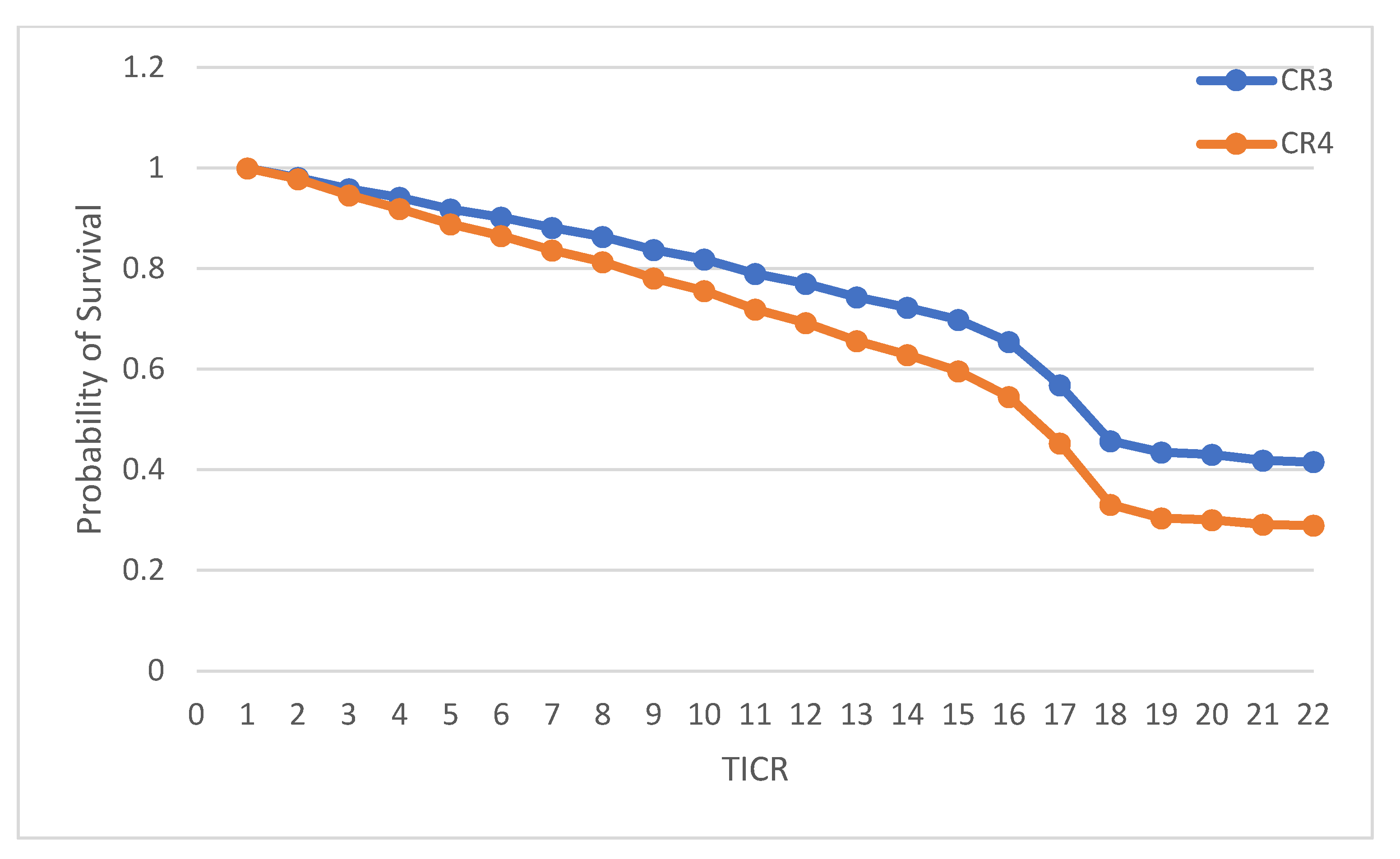
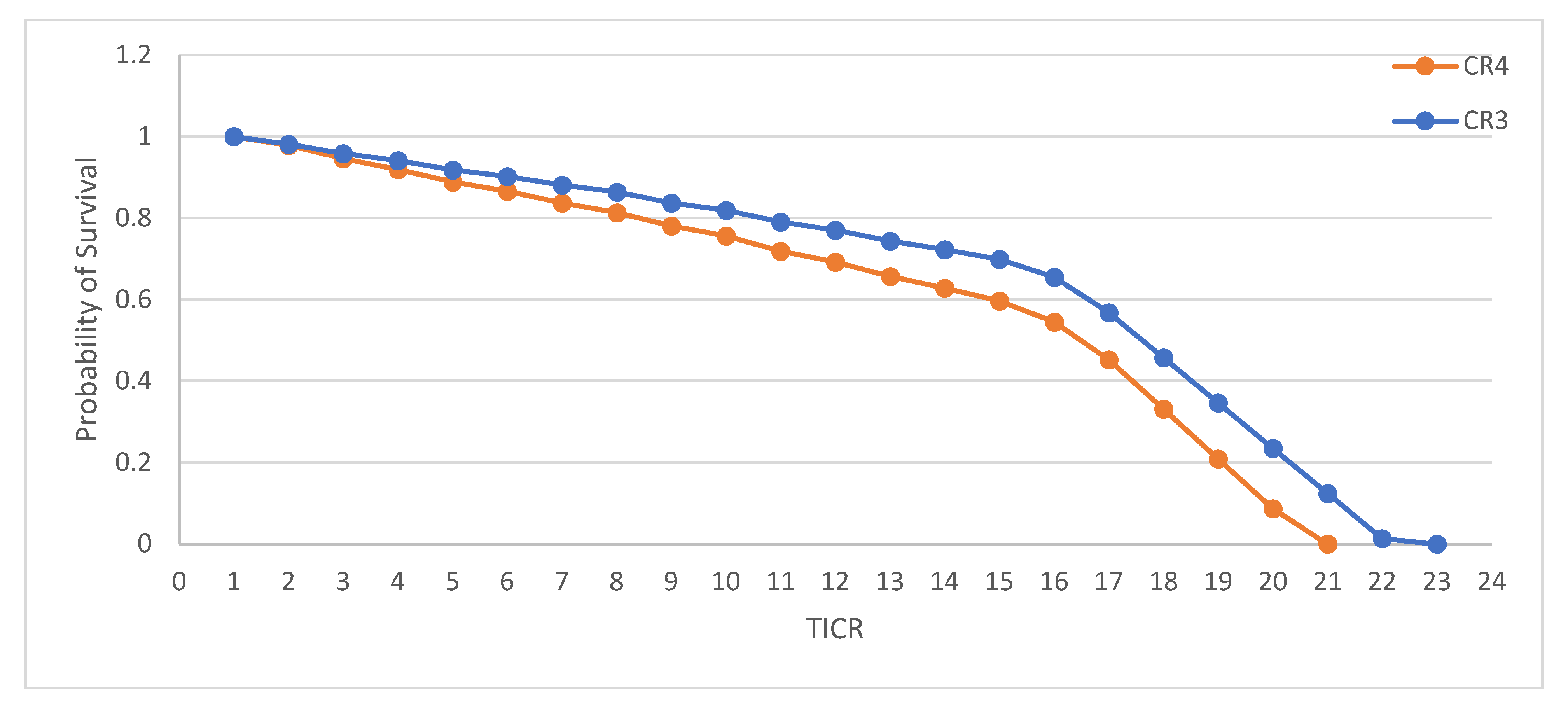
3.1. Survival Curve Estimation
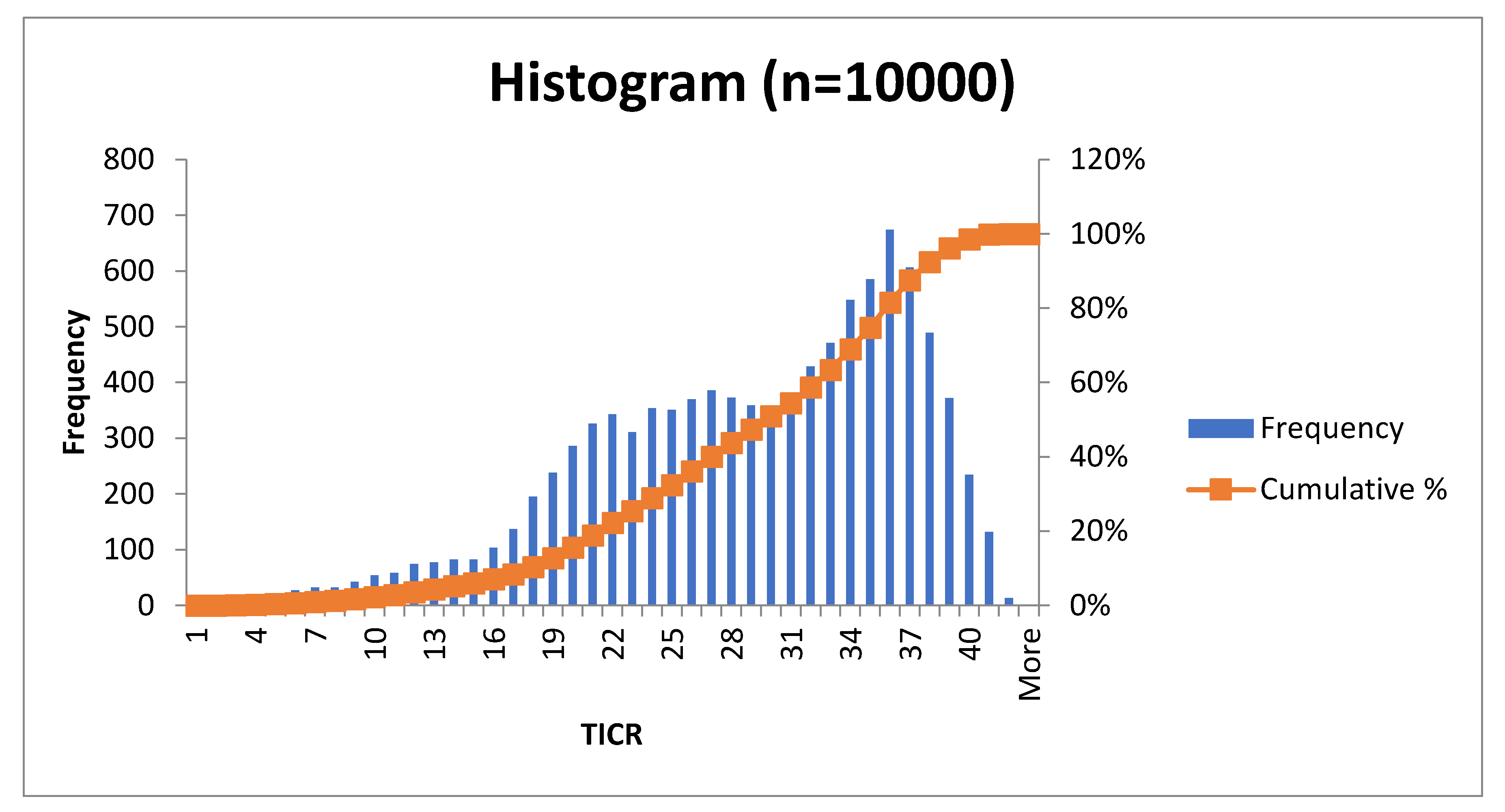
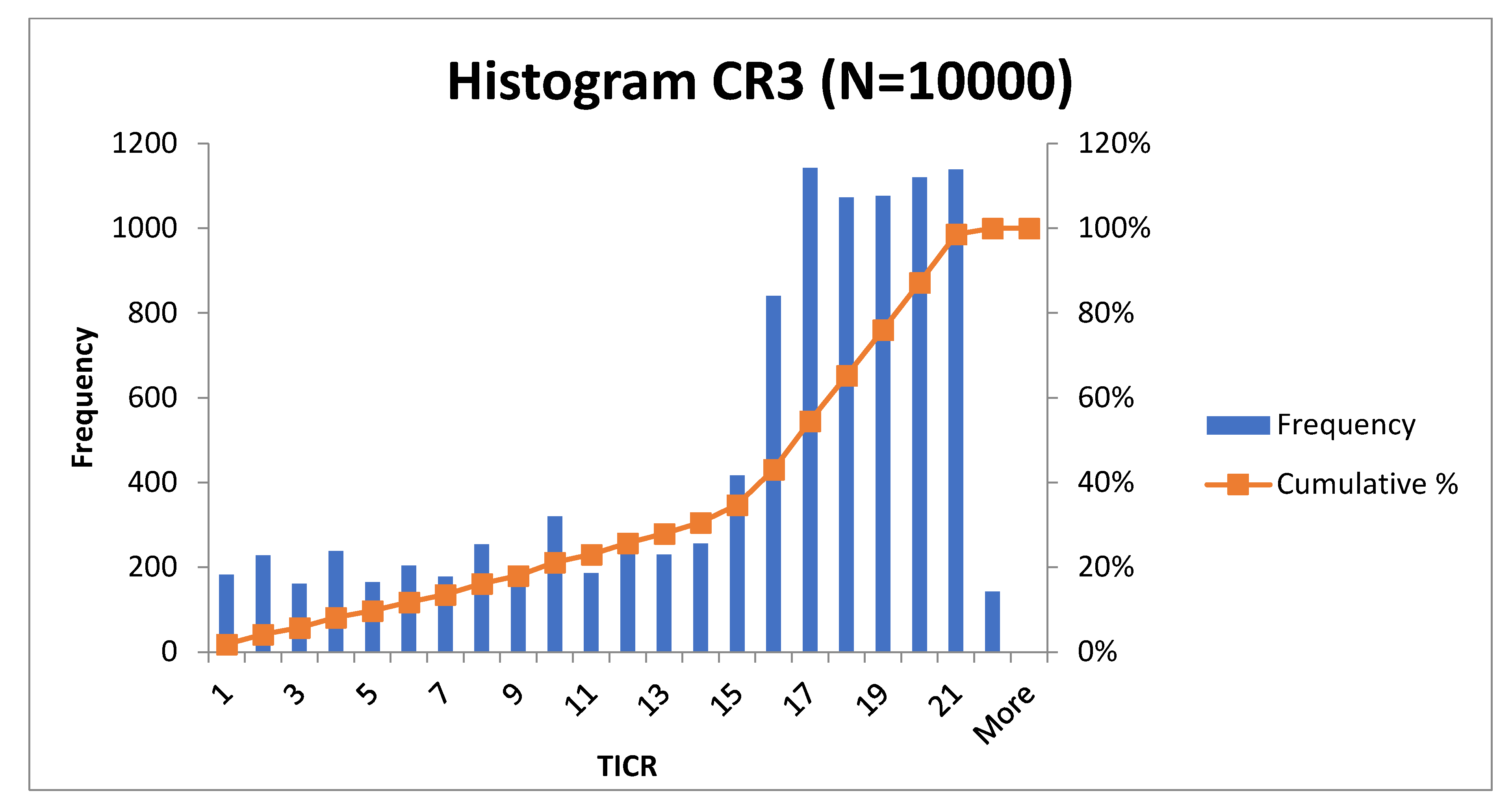
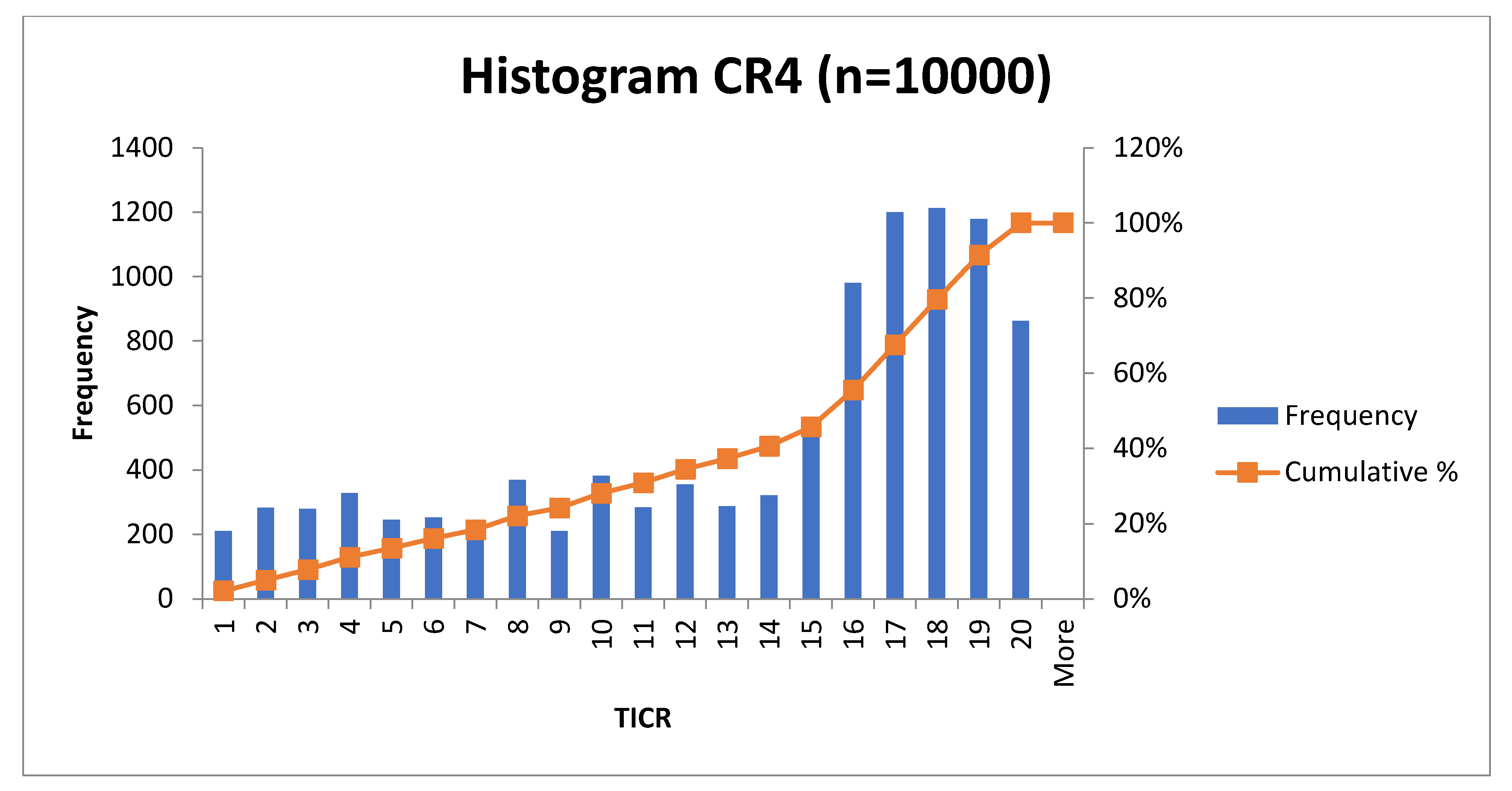
3.2. Monte Carlo Simulation of RUL Distribution
3.3. Calculation of RUL Extension VoI
4. Discussion
5. Conclusions
Author Contributions
Funding
Data Availability Statement
Conflicts of Interest
References
- Bridges. ASCE’s 2017 Infrastructure Report Card. Available online: https://www.infrastructurereportcard.org/cat-item/bridges/ (accessed on 6 September 2020).
- Strong Infrastructure and a Healthy Economy Require Federal Investment. House Budget Committee Democrats. Available online: https://budget.house.gov/publications/report/strong-infrastructure-and-healthy-economy-require-federal-investment (accessed on 30 March 2020).
- World Economic Forum, Strategic Infrastructure 2014. Available online: http://wef.ch/1rM4jzw (accessed on 30 March 2020).
- Hoult, N.A.; Glisic, B. Editorial: Structural Health Monitoring of Bridges. Front. Built Environ. 2020, 6, 17. [Google Scholar] [CrossRef]
- Cawley, P. Structural health monitoring: Closing the gap between research and industrial deployment. Struct. Health Monit. 2018, 17, 1225–1244. [Google Scholar] [CrossRef]
- Limongelli, M.P.; Omenzetter, P.; Yazgan, U.; Soyoz, S. Quantifying the value of monitoring for post-earthquake emergency management of bridges. IABSE Symp. Rep. 2017, 109, 3238–3245. [Google Scholar] [CrossRef]
- Pozzi, M.; Kiureghian, A.D. Assessing the value of information for long-term structural health monitoring. In Health Monitoring of Structural and Biological Systems 2011; International Society for Optics and Photonics; SPIE: Bellingham, WA, USA, 2011; p. 79842W. [Google Scholar] [CrossRef]
- Thöns, S. On the Value of Monitoring Information for the Structural Integrity and Risk Management. Comput.-Aided Civ. Infrastruct. Eng. 2018, 33, 79–94. [Google Scholar] [CrossRef]
- Zonta, D.; Glisic, B.; Adriaenssens, S. Value of information: Impact of monitoring on decision-making. Struct. Control Health Monit. 2014, 21, 1043–1056. [Google Scholar] [CrossRef]
- Special Issue: A Value of Information Perspective. Struct. Health Monit. 2022, 21, 3. [CrossRef]
- Limongelli, M.P.; Previtali, M.; Cantini, L.; Carosio, S.; Matos, J.C.; Isoird, J.M.; Wenzel, H.; Pellegrino, C. Lifecycle management, monitoring and assessment for safe large-scale infrastructures: Challenges and needs. ISPRS-Int. Arch. Photogramm. Remote Sens. Spat. Inf. Sci. 2019, XLII-2/W11, 727–734. [Google Scholar] [CrossRef]
- Bolognani, D.; Verzobio, A.; Tonelli, D.; Cappello, C.; Glisic, B.; Zonta, D. An application of prospect theory to a SHM-based decision problem. In Health Monitoring of Structural and Biological Systems 2017; International Society for Optics and Photonics; SPIE: Bellingham, WA, USA, 2017; p. 101702G. [Google Scholar] [CrossRef]
- Bolognani, D.; Verzobio, A.; Tonelli, D.; Cappello, C.; Glisic, B.; Zonta, D.; Quigley, J. IWSHM 2017: Quantifying the benefit of structural health monitoring: What if the manager is not the owner? Struct. Health Monit. 2018, 17, 1393–1409. [Google Scholar] [CrossRef]
- Cappello, C.; Zonta, D.; Glišić, B. Expected Utility Theory for Monitoring-Based Decision-Making. Proc. IEEE 2016, 104, 1647–1661. [Google Scholar] [CrossRef]
- Zhang, W.-H.; Lu, D.-G.; Qin, J.; Thöns, S.; Faber, M.H. Value of information analysis in civil and infrastructure engineering: A review. J. Infrastruct. Preserv. Resil. 2021, 2, 16. [Google Scholar] [CrossRef]
- Thomson, D.J. The economic case for service life extension of structures using structural health monitoring based on the delayed cost of borrowing. J. Civil Struct. Health Monit. 2013, 3, 335–340. [Google Scholar] [CrossRef]
- Morgan, C.J.; Sparling, B.F.; Wegner, L.D. Use of structural health monitoring to extend the service life of the Diefenbaker Bridge. J. Civil Struct. Health Monit. 2022, 12, 913–929. [Google Scholar] [CrossRef]
- Long, L.; Alcover, I.F.; Thons, S. Quantification of the posterior utilities of SHM campaigns on an orthotropic steel bridge deck. In Proceedings of the 12th International Workshop on Structural Health Monitoring: Enabling Intelligent Life-Cycle Health Management for Industry Internet of Things (IIOT), IWSHM 2019, Stanford, CA, USA, 10–12 September 2019; Structural Health Monitoring 2019. pp. 1504–1511. [Google Scholar] [CrossRef]
- Pasquier, R.; Goulet, J.A.; Acevedo, C.; Smith, I.F. Improving Fatigue Evaluations of Structures Using In-Service Behavior Measurement Data. J. Bridge Eng. 2014, 19, 04014045. [Google Scholar] [CrossRef]
- Bakht, B.; Mufti, A. Evaluation of one hundred and one instrumented bridges suggests a new level of inspection should be established in the bridge design codes. J. Civil Struct. Health Monit. 2018, 8, 3. [Google Scholar] [CrossRef]
- U.S. Department of Transportation, Federal Highway Administration. Recording and Coding Guide for the Structure Inventory and Appraisal of the Nation’s Bridges; U.S. Department of Transportation, Federal Highway Administration: Washington, DC USA, 1995. Available online: http://purl.access.gpo.gov/GPO/LPS112587":["purl.access.gpo.gov"]} (accessed on 3 January 2020).
- 23 CFR § 650.315. Available online: https%3A%2F%2Fwww.govinfo.gov%2Fapp%2Fdetails%2FCFR-2020-title23-vol1%2FCFR-2020-title23-vol1-sec650-315 (accessed on 12 November 2020).
- National Bridge Inventory-Bridge Inspection-Safety-Bridges & Structures-Federal Highway Administration. Available online: https://www.fhwa.dot.gov/bridge/nbi.cfm (accessed on 31 January 2021).
- Babanajad, S.; Bai, Y.; Wenzel, H.; Wenzel, M.; Parvardeh, H.; Rezvani, A.; Zobel, R.; Moon, F.; Maher, A. Life Cycle Assessment Framework for the U.S. Bridge Inventory. Transp. Res. Rec. 2018, 2672, 82–92. [Google Scholar] [CrossRef]
- Kumar, R.; de Oliveira, J.L.M.; Schultz, A.; Marasteanu, M. Remaining Service Life Asset Measure, Phase 1. Minnesota Department of Transportation, Report, July 2018. Available online: http://conservancy.umn.edu/handle/11299/200642 (accessed on 6 March 2023).
- Fleischhacker, A.; Ghonima, O.; Schumacher, T. Bayesian Survival Analysis for US Concrete Highway Bridge Decks. J. Infrastruct. Syst. 2020, 26, 04020001. [Google Scholar] [CrossRef]
- Ayyub, B.M. Risk Analysis in Engineering and Economics; Chapman and Hall/CRC: Boca Raton, FL, USA, 2014. [Google Scholar] [CrossRef]
- Fagbamigbe, A.F.; Idemudia, E.S. Survival analysis and prognostic factors of timing of first childbirth among women in Nigeria. BMC Pregnancy Childbirth 2016, 16, 102. [Google Scholar] [CrossRef] [PubMed]
- Ahmad, T.; Munir, A.; Bhatti, S.H.; Aftab, M.; Raza, M.A. Survival analysis of heart failure patients: A case study. PLoS ONE 2017, 12, e0181001. [Google Scholar] [CrossRef] [PubMed]
- Aalen, O.; Borgan, O.; Gjessing, H. Survival and Event History Analysis: A Process Point of View; Springer: New York, NY, USA, 2008. [Google Scholar]
- Gensheimer, M. MGensheimer/Nnet-Survival. 3 June 2020. Available online: https://github.com/MGensheimer/nnet-survival (accessed on 11 June 2020).
- Valkonen, A. Exploring Structural Health Monitoring Value of Information based on Remaining Useful Life Extension Potential. Ph.D. Dissertation, Princeton University, Princeton, NJ, USA, 2023. Available online: https://dataspace.princeton.edu/handle/88435/dsp019019s5734 (accessed on 8 September 2023).
- Non-Uniform Random Variate Generation. Available online: http://www.nrbook.com/devroye/ (accessed on 13 December 2022).
- Ross, S. (Ed.) Chapter 4-Generating Discrete Random Variables. In Simulation, 5th ed.; Academic Press: Cambridge, MA, USA, 2013; pp. 47–68. [Google Scholar] [CrossRef]
- LTBP InfoBridge. Available online: https://infobridge.fhwa.dot.gov/ (accessed on 19 December 2022).
- Kelley, R. A Process for Systematic Review of Bridge Deterioration Rates. Michigan Department of Transportation, March 2016. Available online: https://www.michigan.gov/-/media/Project/Websites/MDOT/Programs/Bridges-and-Structures/BOBS/BOBS-2/Process-for-Systematic-Review-of-Bridge-Deterioration-Rates.pdf?rev=f4a9ee454dac4df1932211761afb0e2d (accessed on 7 March 2023).
- Benefit-Cost Analysis Guidance for Discretionary Grant Programs|US Department of Transportation. Available online: https://www.transportation.gov/mission/office-secretary/office-policy/transportation-policy/benefit-cost-analysis-guidance (accessed on 7 March 2023).
- NJDOT Cost Estimating Guideline. February 2019. Available online: https://www.state.nj.us/transportation/capital/pd/documents/Cost_Estimating_Guideline.pdf (accessed on 7 March 2023).
- FRB H15: Data Download-Download. Available online: https://www.federalreserve.gov/datadownload/Download.aspx?rel=H15&series=b56abb6d9cc35f28ccf86b8a0188e948&lastObs=&from=02/15/1977&to=03/09/2023&filetype=spreadsheetml&label=include&layout=seriescolumn (accessed on 11 March 2023).


| Rating | Condition Description |
|---|---|
| 9 | Excellent Condition |
| 8 | Very Good Condition |
| 7 | Good Condition |
| 6 | Satisfactory Condition |
| 5 | Fair Condition |
| 4 | Poor Condition |
| 3 | Serious Condition |
| 2 | Critical Condition |
| 1 | “Imminent” Failure Condition |
| 0 | Failed Condition—out of service—beyond corrective action |
| Description of Covariate | Abbreviation | Range of Values |
|---|---|---|
| Average Daily Truck Traffic | ADTT | [0.56595] |
| Climatic Region | ClimaticRegion | “Region 2—very hot”; “Region 3—hot”; “Region 4—average”; “Region 5—cold “; “Region 6—very cold”; “Region 7—extremely cold”; “Region 8—subarctic”; “Region 9—average marine”; “Region 10—hot marine”. |
| Condition Rating | CR | CR3, CR4, CR5, CR6, CR7, CR8, CR9. |
| Deck Protection Type | DeckProt | “None”; “Epoxy-coated reinforcing”; “Galvanized reinforcing”; “Other coated reinforcing”. “Cathodic protection”; “Polymer impregnated”; “Internally sealed”; “Unknown”; “Other”. |
| Deck Type | DeckType | “Concrete cast-in-place”; “Concrete precast panels”. |
| Distance to Sea Water | SeaDist | “Sea Less than 3 km Away”; “Sea More Than 3 km Away”. |
| Functional Classification (NBI Item 26) | FunctClass | “Rural”; “Urban”. |
| Maintenance Responsibility | MaintResp | “State highway agency”; “County highway agency”; “Town/township highway agency”, “City/municipal highway agency”, “Private (other than railroad)”; “State toll authority”. |
| Structural Type | StructType | “Concrete-simple span”; “Concrete-continuous”; “Steel-simple span”; “Steel-continuous”; “Prestressed concrete-simple span”; “Prestressed concrete-continuous”. |
| NBI Structure Number | 1618150 |
| Location | Wayne Township, NJ, USA |
| Route | US202 |
| Year Built | 1983 |
| Deck Area, sq. ft. | 52,937.7 |
| Latitude, | 40.91485 |
| Longitude | −74.26529 |
| Description of Covariate | Abbreviation | Range of Values |
|---|---|---|
| Average Daily Truck Traffic (recording period used to calculate the average: year 2020) | ADTT | 3335 |
| Climatic Region | ClimaticRegion | “Region 5-cold “; |
| Deck Condition Rating (Current) | CR | CR6 |
| Deck Protection Type | DeckProt | “Epoxy-coated reinforcing”; |
| Deck Type | DeckType | “Concrete cast-in-place”; |
| Distance to Sea Water | SeaDist | “Sea More Than 3 km Away” |
| Functional Classification (NBI Item 26) | FunctClass | “Urban” |
| Maintenance Responsibility | MaintResp | “State highway agency”; |
| Structural Type | StructType | “Steel-simple span” |
| Project Category | Units Used for Calculations | Median Cost per Unit | Low Cost | Average Cost | High Cost |
|---|---|---|---|---|---|
| Bridge Deck Replacement | Square Foot | USD 320 | USD 150 | USD 380 | USD 730 |
| Bridge Superstructure Replacement | Square Foot | USD 400 | USD 230 | USD 530 | USD 1300 |
| Bridge Replacement | Square Foot | USD 1800 | USD 750 | USD 1900 | USD 3500 |
| Culver Replacement | Square Foot | USD 2700 | USD 1300 | USD 2300 | USD 3300 |
| Low Cost | Median Cost | Average Cost | High Cost | |
|---|---|---|---|---|
| Bridge Deck Replacement Cost (Dollars per Square Foot) | 181.5 | 387.2 | 459.8 | 883.3 |
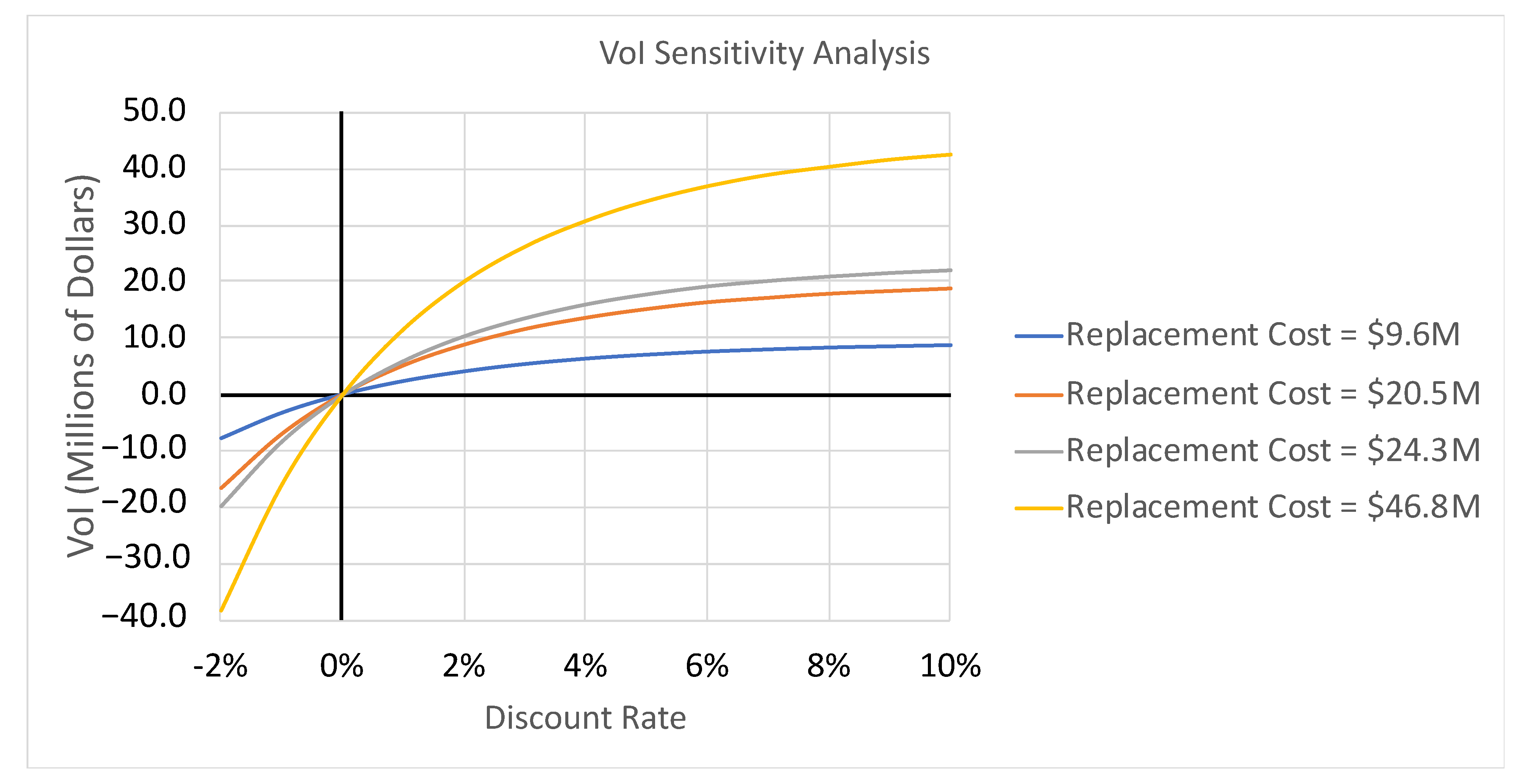
| Total Replacement Cost (Millions of Dollars) | 9.6 | 20.5 | 24.3 | 46.8 |
| Low Cost | Median Cost | Average Cost | High Cost | |
|---|---|---|---|---|
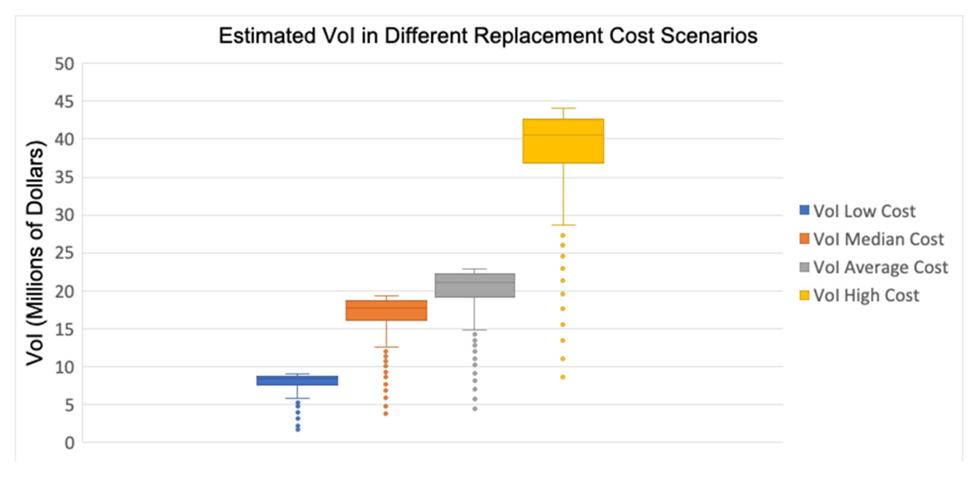
| Max VoI (Millions of Dollars) | 9.0 | 19.3 | 22.9 | 44.0 |
| Min VoI (Millions of Dollars) | 1.2 | 2.6 | 3.1 | 5.9 |
| Average VoI (Millions of Dollars) | 8.0 | 17.1 | 20.3 | 39.0 |
Disclaimer/Publisher’s Note: The statements, opinions and data contained in all publications are solely those of the individual author(s) and contributor(s) and not of MDPI and/or the editor(s). MDPI and/or the editor(s) disclaim responsibility for any injury to people or property resulting from any ideas, methods, instructions or products referred to in the content. |
© 2023 by the authors. Licensee MDPI, Basel, Switzerland. This article is an open access article distributed under the terms and conditions of the Creative Commons Attribution (CC BY) license (https://creativecommons.org/licenses/by/4.0/).
Share and Cite
Valkonen, A.; Glisic, B. Structural Health Monitoring-Based Bridge Lifecycle Extension: Survival Analysis and Monte Carlo-Based Quantification of Value of Information. Infrastructures 2023, 8, 158. https://doi.org/10.3390/infrastructures8110158
Valkonen A, Glisic B. Structural Health Monitoring-Based Bridge Lifecycle Extension: Survival Analysis and Monte Carlo-Based Quantification of Value of Information. Infrastructures. 2023; 8(11):158. https://doi.org/10.3390/infrastructures8110158
Chicago/Turabian StyleValkonen, Antti, and Branko Glisic. 2023. "Structural Health Monitoring-Based Bridge Lifecycle Extension: Survival Analysis and Monte Carlo-Based Quantification of Value of Information" Infrastructures 8, no. 11: 158. https://doi.org/10.3390/infrastructures8110158