
Ensemble Learning Approach for Developing Performance Models of Flexible Pavement


Department of Civil and Environmental Engineering, Florida State University, College of Engineering, 2525 Pottsdamer Street, Tallahassee, FL 32310, USA
*
Author to whom correspondence should be addressed.
Infrastructures 2024, 9(5), 78; https://doi.org/10.3390/infrastructures9050078
Submission received: 3 April 2024
/
Revised: 20 April 2024
/
Accepted: 23 April 2024
/
Published: 25 April 2024
(This article belongs to the Section Infrastructures and Structural Engineering)
Abstract
:This research utilizes the Long-Term Pavement Performance database, focusing on devel-oping a predictive model for flexible pavement performance in the Southern United States. Analyzing 367 pavement sections, this study investigates crucial factors influencing asphaltic concrete (AC) pavement deterioration, such as structural and material components, air voids, compaction density, temperature at laydown, traffic load, precipitation, and freeze–thaw cycles. The objective of this study is to develop a predictive machine learning model for AC pavement wheel path cracking (WpCrAr) and the age at which cracking initiates (WpCrAr) as performance indicators. This study thoroughly investigated three ensemble machine learning models, including random forest, extremely randomized trees (ETR), and extreme gradient boosting (XGBoost). It was observed that XGBoost, optimized using Bayesian methods, emerged as the most effective among the evaluated models, demonstrating good predictive accuracy, with an R2 of 0.79 for WpCrAr and 0.92 for AgeCrack and mean absolute errors of 1.07 and 0.74, respectively. The most important features influencing crack initiation and progression were identified, including equivalent single axle load (ESAL), pavement age, number of layers, precipitation, and freeze–thaw cycles. This paper also showed the impact of pavement material combinations for base and subgrade layers on the delay of crack initiation.
1. Introduction
In an effort to improve the development of pavement performance models, the number of studies has increased on the application of data-driven approaches, especially, the use of machine learning techniques [1,2,3]. These efforts have also been enhanced with the availability of rich pertinent databases such as the Long-Term Pavement Performance (LTPP) database, maintained by the Federal Highway Administration in the United States. The LTPP database contains information regarding construction, structure, traffic, and performance over time, as well as geological climate data. Studies showed that machine learning models outperform traditional mathematical models by uncovering and explaining correlation patterns among various input features in relation to the target variable, thereby offering greater efficiency, speed, and analytical accuracy [4,5,6,7,8,9].
Roadway pavements are subject to deterioration due to a variety of factors, such as environmental disasters, aging, design flaws, etc. Studies demonstrate that pavement deterioration is primarily influenced by structural and traffic-related factors [10,11,12]. Additionally, environmental factors intensify several of these deterioration mechanisms, including traffic fatigue and surface temperature stresses, which have an impact on the functionality and serviceability of highway networks [13]. For instance, precipitation penetration can significantly impact pavement integrity by dissolving the base material underneath the asphalt surface, which leads to cracking propagation [14,15]. Specific cases of pavement failure have been linked to insufficient drainage systems, high traffic volumes, improper material gradation, and poor subgrade soil [16]. Furthermore, natural disasters (e.g., hurricanes and earthquakes) or human errors (e.g., vehicle collisions) pose additional challenges to maintaining pavement section integrity. It is imperative to comprehend and address these factors affecting deterioration to extend the lifespan of pavements and ensure their performance efficiency.
A geospatial hotspot analysis using decision tree models suggested that fatigue cracking is highly correlated with truck traffic loads [17]. The present research study also considers the effect of truckloads to find their direct impact on asphalt cracking. By incorporating integral channel features and a random forest algorithm, the detection framework successfully captures the inherent structure of road cracks, which improves the traditional crack detection approach [18,19,20]. Another random forest study on the LTPP database demonstrated that seal coat treatments contribute to the reduction of pavement surface cracking, with pavement condition and seal coat thickness proving critical for rutting and International Roughness Index (IRI) performance [21,22]. The significant impact of mixture gradation and aggregate-specific gravity on alligator cracking in asphaltic concrete (AC) pavement has been identified using random forest models [23]. Machine learning algorithms, including extreme gradient boosting (XGBoost) and random forest, have been applied to correlate surface temperature and AC layer thickness to its modulus [24].
Temperature has a more significant positive correlation influence on the rutting depth of asphalt pavement than other variables, such as the number of load cycles and mix design considerations [25]. The results from the boosting machine learning model found that traffic volume, environmental conditions, and service age substantially influence the performance of pavement overlays, while both rutting and transverse cracking displayed a heightened sensitivity to the state of the pavement before the overlay construction [26]. Annual climatic transitions cause seasonal alterations due to the freeze–thaw cycles of underlying soils. As the temperature rises, the soil thaws from the surface down, trapping water between the pavement and the still-frozen soil, leading to a compromised foundation [27]. Considering the unique material types and needs prevalent in each specific region in the U.S., this research study narrows its scope focusing on the southern states. Compared to the previous similar literature, this study incorporates a combination of mechanical factors affecting pavement cracking, such as density, air voids, and layer properties, etc. One instance that the current study considers is the significance of maintenance and rehabilitation tasks, which incorporate information related to various phases in the pavement’s lifecycle. This information is characterized by unique construction numbers within the LTPP database, reflecting changes in the number, thickness, and material properties of various layers.
Many of the recently developed models for pavement performance are based on empirical in-service data [28,29,30,31,32]. Based on the reviews of prior studies as presented above, it was observed that there is a need to include more pertinent data from the construction phase of the pavement with the in-service data when modeling the pavement performance. Transportation agencies store a significant quantity of data throughout various stages in the life cycle of an asset, from design, surveying, and construction to maintenance and rehabilitation. As an asset advances through its life cycle, the accumulation of digital information correspondingly increases. However, the stored information is often subject to segmentation and may become underutilized or even lost during transitions between project phases, frequently due to the limitations imposed by traditional workflows [33,34]. Therefore, from the viewpoint of this study, it is critical to integrate all the gathered information within an asset management model, making it beneficial to all stakeholders to enhance the performance of the infrastructure system. Crucial information during the design and construction phases could subsequently be used in maintenance, operation, and rehabilitation phases. Despite recent advancements, understanding how the quality of construction or structural changes in maintenance and rehabilitation practices impact the long-term performance of pavements remains an unexplored area of study.
As shown in Table 1, comparing to prevailing prediction models of pavement deterioration that predominantly employ pavement age as the sole predictor, researchers have begun proposing various ML-based deterioration models for pavement based on various predictors [35,36,37,38]. All the listed models incorporate various features, such as traffic load, climate factors, and structural characteristics, offering important insights into pavement behavior. While traditional analytical and empirical pavement performance models have provided valuable information, especially concerning fatigue cracking, they often fail to accurately capture the complex and dynamic connections that define pavement cracking mechanisms.
This study aims to leverage various ensemble learning techniques to develop robust deterioration models that can comprehensively analyze pavement’s long-term performance throughout its lifecycle and forecast the age of cracking initiation, as well as wheel path crack values. The pertinent data, including various structural details, environmental factors, traffic loads, construction quality, and maintenance and rehabilitation changes, collected from LTPP program were processed and served as the input features. The research effort employed three optimization algorithms, namely, random search, grid search, and Bayesian, to find the most suitable approach for each machine learning model. Additionally, the subgrade and base layer material data incorporation impact on the asphalt performance prediction has been investigated. The objective of this research is to develop a highly precise performance model for asphalt concrete pavement that can predict not only the occurrence of wheel path cracking but also the age at which this cracking begins. This study also will identify the most important factors affecting pavement deterioration using both performance indicators.
In the following sections, the steps taken in the data collection and processing are discussed, including the database tables and relationships, as well as the specific features selected for the models. The following section describes the underlying attributes of the proposed methodology, specifically, the random forest, extremely randomized trees, and extreme gradient boosting models. Next, the results are presented for each of the three models, including the training and testing steps, as well as the accuracy values obtained. A discussion of the results is then presented, followed by the final section on the conclusion and suggestions for future research.
2. Data Processing
The FHWA’s LTPP database has pavement performance data of 2981 sections, collected over three decades. The LTPP database is publicly accessible to monitor the location, quantities, types, and severity of pavement distress for each section. All sections are grouped by LTPP section identifiers, e.g., SHRP_ID, STATE_CODE, and CONSTRUCTION_NO. The authors classified selected features from the LTPP tables into five categories, including (1) pavement structure and construction, (2) construction quality, (3) climate, (4) traffic, and (5) in-service. In this study, 367 unique pavement sections in the southern region of the U.S., and 2578 observations were identified. The research is focused on the southern United States, where the distinctive climatic and infrastructural factors are examined. For instance, southern states are characterized by higher temperatures and fewer freezing cycles, in contrast to the northern states, where more frequent freezing cycles occur. These climatic differences significantly influence pavement performance and durability. This geographical focus enables a thorough examination of how regional environmental conditions influence road infrastructure. Due to the diverse regional characteristics in the United States, including variations in structural design, material properties, and distinct environmental conditions, the authors chose to focus on the sections that are located in the southern U.S., including Alabama, Arkansas, Florida, Georgia, Louisiana, Mississippi, New Mexico, Oklahoma, South Carolina, Tennessee, and Texas, as mapped in Figure 1.
A short description, definition of acronyms, range of values, and units of the features employed in this study are provided in Table 2.
The related LTPP tables were extracted using U.S. customary units into a singular Microsoft Access database, which comprises attributes from six key LTPP tables, including Analysis_Tst_AC; Mon_Dis_AC_Rev; Tst_L05B; AC_Density_Meas; Merra_Temp_Precipitation; and TRF_Trend. Table Analysis_Tst_AC contains relevant construction metrics, including air voids on wheel path sections, voids filled with asphalt, and voids in the mineral aggregate. Mon_Dis_AC_Rev provided cracking data, as well as surface width measurements. The Tst_L05B table detailed the material used for distinct pavement layers within each test section and their relative thickness values. Table AC_Density_Meas provided density values for the top surface layer in each section. Table Merra_Temp_Precipitation supplied environmental attributes, such as precipitation, temperature, and freeze–thaw, for analysis. The TRF_Trend table provided the annual ESAL trend information to represent traffic load for heavy vehicles in classes 4–13. The authors developed an SQL algorithm, as illustrated using the entity relation diagram in Figure 2, to cross-reference all the exported attributes for the selected sections from LTTP by linking their mutual STATE_CODE, SHRP_ID, CONSTRUCTION_NO, LAYER_NO, and SURVEY_DATE values.
As pavement ages, it can lead to a loss of flexibility and resilience, reducing its ability to withstand traffic loads and environmental stressors, and ultimately deteriorating by different types of cracking, especially when no rehabilitation is performed. The equivalent single axle load (ESAL), being one of the main stressors for a pavement section, represents a single pass of a standard axle load (typically 18,000 pounds or 8200 kg), which quantifies the impact of a vehicle on the pavement’s structural integrity. Over time, the cumulative effect of ESAL loads can lead to fatigue cracking, rutting, and other forms of pavement distress.
Among the temperature-related input features, average daily ambient temperature (AvgTmp) could affect the strain on the pavement for a given traffic stress. Therefore, for a given traffic load, the pavement experiences greater stresses and strains in regions with lower average temperatures than it does at higher temperatures, at which the materials are less rigid [42]. Explicitly incorporating AvgTmp into asphalt performance prediction models provides an opportunity to better capture the existing correlation between crack progression and temperature-dependent factors. Asphalt mixture temperature during laydown (SurfTmp) is also crucial, as it affects workability, compaction, and subsequent performance. Proper temperatures at placement enable adequate compaction and avoid distresses like cracking, while excess heat risks bleeding and segregation. The freeze–thaw cycle, indicated by the FrzThaw feature, can also affect the soil underneath the pavement (subgrade materials). When the soil freezes and thaws, it can shift and settle unevenly, leading to a weaker foundation for the pavement, which can cause the pavement to crack under the weight of heavy traffic [43,44]. Precipitation (Precip) infiltration into the subbase can lead to a reduction in the resilient modulus and stripping in asphalt layers (resulting in the loss of adhesion between aggregate and the asphalt binder), which weakens the mechanical properties of the underlying layers [45].
The composition and characteristics of individual layers can contribute significantly to the overall performance of the pavement. One of the primary functions of layering in an AC section is to distribute the loads placed on the pavement surface. More layers can often mean better load distribution, which can reduce the strain and decrease the rate of crack progression, as the surface layer does not bear the entire force from tire pressure directly. To account for maintenance changes in the pavement structure, the number of layers in each construction number (LyrC) has also been taken into consideration as a separate feature. The thicknesses of the subbase layer (SubbTh), base layer (BaTh), original surface layer (OslTh), binder layer (BiTh), and overlay layer (OvrTh) have been considered in the models, as well as the type of materials used for the subgrade and base layer.
AC compaction is a critical process in pavement construction, with a higher density often leading to increased durability and fatigue resistance. Dense asphalt pavements that can better withstand the stresses of traffic loads are less likely to experience fatigue cracking over time and are less permeable, making them more resistant to moisture damage [46]. Air voids in the AC section, represented as the variable AvWp for wheel path air voids, therefore play a critical role in the progression of cracking and the pavement’s overall performance. The content of these air voids is a fundamental property that can directly affect the durability and performance of the pavement. Theoretically, more air voids would mean less asphalt binder and aggregate in the mix, which can reduce the overall strength and durability of the asphalt concrete [47]. Higher air void content can increase moisture susceptibility and accelerate aging, leading to premature cracking [48], but too few voids may also cause pavement distress, such as rutting [49]. Voids mineral aggregate (VMA) refers to the void spaces between compacted aggregates in an asphalt mix that provides room for binder, whereas voids filled asphalt (VFA) represents the percentage of VMA filled by binder versus air voids [50]. This study investigated, separately for each layer, the impact of VFA and VMA percentage on the original surface layer, overlay, and binder layer. The target variables analyzed are the time required for the initial appearance of cracks in a specified pavement section (AgeCrack) and the measured crack length per pavement surface area (WpCrAr).
One of the novel aspects of this research is the consideration of the change in the number of layers for each pavement section, which reflects the chronological sequence of maintenance and rehabilitation construction that has been carried out on the segment, indicated by the construction number (CN1, CN2, and CN3) variable. The input variable for truck loads, as well as the precipitation amount, were estimated from the cumulative ESALs for the respective CN interval. This study also employed a feature selection method to reach a better understanding of the importance of each feature in correlation to the output feature. The scatterplot matrix and mutual information feature selection (MIFS) methods were used for feature selection, which are presented in Figure 3 and Figure 4, respectively. The scatterplot matrix indicates the correlation among the variables, while the MIFS quantifies the mutual dependency between input variables and the output, especially in cases in which the relationship is non-linear [51,52,53].
In the scatterplot matrix, the lower triangle of the plot shows the corresponding regression trendline for each feature pair. Additionally, the Pearson correlation coefficient between each attribute pair is presented using as blue-to-red gradient heat map in the upper triangle of the plot (with blue and red demonstrating the most negative and positive correlations, respectively). Among input features, Age, Precip, LyrC, and FrzThaw have the most significant correlation with WpCrAr (dependent variable). The scatterplot matrix shows considerable intercorrelation between VMA and VFA features for different pavement layers, i.e., the original surface layer, the overlay, and the binder layer. Moreover, the intercorrelation of the AvWp feature with the VMA feature in those layers is also significant. Considering the results of MIFS and the low importance of VMA_Bi, VMA_Ovr, and VFA_Ovr and their higher correlation with their related AvWp features (0.86, 0.91, and 0.79, respectively), the three features were removed from the further analysis to avoid overfitting problems. Furthermore, VMA_Osl has a high correlation with AvWp_Osl (0.81) and was also excluded from the machine learning models.
Using the MIFS helped to reduce dimensionality while preserving the most informative features for developing machine learning models. As Figure 4 suggests, Age, Precip, ESAL, FrzThaw, and BaTh are the top five most influential factors among the input features, whereas VFA_Ovr, VMA_Ovr, VMA_Bi, LyrC, and AvWp_Ovr have the lowest correlation values. In contrast to MIFS, the correlation plot matrix did not identify ESAL as an important feature input. Therefore, employing both methods for feature selection can be a proper strategy because it capitalizes on their complementary strengths. This approach provides a more comprehensive understanding of the intercorrelation between input variable and output feature, ultimately leading to a more robust and accurate machine learning model.
Considering the nominal type of material data, their interpretations through the output of machine learning models such as feature importance analyses are somewhat limited and irrelevant. As shown in Figure 5, the significance of employing material data is to obtain a thorough understanding of the relationship between various material combinations for base and subgrade layers and analyze their impact on the age at which cracking in pavement sections begins.
The 50th percentile value for AgeCrack represents the age by which 50% of the sections started to crack. Therefore, if a material combination has a high 75th percentile AgeCrack value, it means that the majority of sections (75%) took a longer time to start showing cracks, indicating a potentially better performance in terms of durability. Among the material combinations, the sections with open graded, hot laid/fine-grained soils stand out for their remarkable durability, displaying the highest 75th percentile value of 17.25 years. This indicates that the majority of these sections took significantly longer to start cracking compared to other combinations. In addition, this combination also has the highest AgeCrack_Avg of 11.5 years, reinforcing its superior performance. However, the compressed range between the median (50th percentile) and the 75th percentile suggests that the majority of sections start cracking at median age and only a quarter shows higher durability. From a practical point of view, this consistency in the performance can be a useful insight for maintenance planning, as it suggests that once the median service life is reached, the aforementioned pavement sections may need to be monitored more closely for the onset of cracking. This trend is also observed in sections with a gravel base layer paired with both coarse- and fine-grained subgrade layers, in which the majority of sections begin exhibiting cracking only beyond the median age of cracking. Similarly, the crushed stone/coarse-grained soils combination also showed high resistance to cracking initiation, with a 75th percentile value of 11.30 years, making it another robust choice for pavement materials. On the other hand, combinations involving fine-grained soils as base material, whether paired with coarse-grained or fine-grained subgrade materials, exhibit a much earlier onset of cracking deterioration, having lower median AgeCrack values of 0.87 and 3.33 years, respectively. A combination of sand asphalt/coarse-grained soils for base and subgrade layers has the lowest 50th percentile values of 0.25 and 0.34 years, respectively, indicating early signs of cracking. The difference in AgeCrack values with different pavement materials indicates a strong relationship between material selection and pavement durability. This variability suggests that including various material types for base and subgrade layer in the input database of machine learning models is not only reasonable but necessary for capturing the full spectrum of factors affecting pavement longevity. Further exploration of these datapoints, alongside other input features, could significantly enhance the predictive maintenance of roadways and optimize material selection in the design phase.
Recognizing the significant impact of material selection on pavement durability, as discussed above, underscores the necessity to incorporate this critical factor into our machine learning regression models. The distinct performance metrics observed across various combinations of materials for base and subgrade layers—particularly the correlation of specific material types with the cracking initiation—highlight the complexity of predicting pavement longevity. To effectively model these dynamics and improve the predictive accuracy of our models, the implementation of one-hot encoding emerges as a pivotal strategy to address this challenge. By transforming categorical material data into a format that is interpretable by machine learning algorithms, we aim to bridge the gap between qualitative material attributes and quantitative model inputs for pavement performance models.
Using one-hot encoding transformation, pavement material data were embedded into the input database to help provide more insight into the machine learning models from a physical perspective. In this case, the “BaMat” and “SubgrMat” variables are categorical, representing different types of materials used for base and subgrade layers. Using this method, each unique category becomes a separate feature with a binary value (0 or 1). This binary matrix format allows models to handle nominal material data that lack any inherent order, weighting, or intrinsic relationships. By converting the diverse material characteristics into a binary matrix, the models were able to discern patterns and relationships that were not previously investigated, leading to a more precise and reliable prediction accuracy. This methodological enhancement underscores the importance of feature engineering in improving the efficacy of machine learning models, especially in complex domains in which material properties play a crucial role. Figure 6 illustrates the methodological approach applied to the LTPP material database using the one-hot encoding method.
The required computing resource to process such a big database is an important consideration for the application of any machine learning methodologies. Table 3 outlines the hardware specifications of the high-performance computing (HPC) resource utilized for all the machine learning computations. The allocated computing node comprises an Intel Xeon (R) E5 2670 CPU operating at 2.60 GHz with 32 cores paired with 32 GB of DDR4 RAM at 2600 MT/s. The table provided below is crucial for demonstrating both the computational capability and the economic viability of using high-performance computing resources for sophisticated data processing tasks, especially for large-scale projects anticipated at Departments of Transportation (DOTs).
3. Methodology
This section of the paper presents the overall methodology, the machine learning algorithm frameworks, optimization methods, and evaluation criteria employed to develop and fine-tune the model for processing the LTPP data. As shown in Figure 7, the research methodology begins gathering and cleaning up the data, as well as data visualization. The innovative distinction of this framework from previous models lies in its utilization of the one-hot encoding method to transform pavement material data into binary features, as well as capturing structural changes during multiple maintenance and rehabilitation phases. Subsequently, machine learning models were developed, optimized, and compared. The exploration process aimed to uncover the most important features and correlations existing between long-term wheel path cracking and the age of cracking initiation (as dependent) and various features (as independent).
3.1. Machine Learning Models
Ensemble models, such as random forest, extremely randomized trees, and extreme gradient boosting (XGBoost), aggregate predictions from several models to provide a more robust prediction. The ensemble models are beneficial for many machine learning applications due to their diversity, which allows them to better handle missing data, reduce overfitting, and improve the models’ capacity to generalize. Following the initial data selection from the LTPP database, pre-processing techniques, including data cleaning, filtering, merging, and normalization, were applied to prepare the final input dataset for the machine learning models. Choosing an extensive range of machine learning algorithms is beneficial, as it allows for the exploration of various models to find the most effective technique to explain crack progression based on the attributes described above.
3.1.1. Random Forest
Random forest decision tree models can evaluate the importance of each input feature and their contribution to predicting testing accuracy. Random forests are often considered to be versatile due to their ability to handle a wider range of problems because they can use a wider range of splitting rules, feature selection methods, and reliability to work with imbalanced data. Random forest operates by constructing a multitude of decision trees during training, with each tree grown independently to its full capacity on a different bootstrapped subset of the data. Therefore, it does not utilize a global mathematical objective function that guides the training of individual trees. Instead, the random forest algorithm leverages the collective decision-making of the entire ensemble of trees to improve predictive accuracy and robustness. The aggregation of these independent models, typically by averaging their predictions, is what reinforces random forest’s performance on regression tasks. Figure 8 shows the decision tree procedure of the random forest models.
The random forest regression model architecture could be utilized using the algorithm shown in Algorithm 1.
| Algorithm 1 Pseudocode algorithm for random forest |
| Precondition: A training set S:= (X_train, y_train), features F, and number of trees in forest B. 1 function RandomForestRegression(S, F, B) 2 H ← empty list//This will store all the individual trees 3 for i ∈ 1, …, B do 4 S(i) ← BootstrapSample(S)//Generate a bootstrap sample from the original dataset 5 tree ← BuildDecisionTree(S(i), F) 6 Append tree to H 7 end for 8 return H//Return the ensemble of trees 9 end function 10 function BootstrapSample(S) 11 sample ← empty list 12 for i ∈ 1, …, length(S) do 13 s ← Randomly select an instance from S with replacement 14 Append s to sample 15 end for 16 return sample 17 end function 18 function BuildDecisionTree(S, F) 19 if StoppingCriteriaMet(S) then 20 return a leaf node with the mean of y-values in S 21 end if 22 23 best_split ← FindBestSplit(S, F) 24 left_subtree ← BuildDecisionTree(S where instances match left side of best_split, F) 25 right_subtree ← BuildDecisionTree(S where instances match right side of best_split, F) 26 27 return a node representing best_split with left_subtree and right_subtree as children 28 end function 29 function FindBestSplit(S, F) 30 best_score ← infinity//Initialize with a very high value since we’re looking to minimize error for regression 31 best_feature ← null 32 best_threshold ← null 33 34 for each feature f in F do 35 for each value v in f do 36 left_subset, right_subset ← SplitData(S, f, v) 37 current_score ← CalculateMSE(left_subset) + CalculateMSE(right_subset) 38 39 if current_score < best_score then 40 best_score ← current_score 41 best_feature ← f 42 best_threshold ← v 43 end if 44 end for 45 end for 46 47 return best_feature and best_threshold as the best split 48 end function 49 function CalculateMSE(subset) 50 mean_value ← Calculate mean of y-values in subset 51 mse ← Mean of (y_i - mean_value)^2 for each instance in subset 52 return mse 53 end function |
3.1.2. Extremely Randomized Trees (Extra Trees)
The extra trees algorithm leverages multiple decision trees and randomness to improve model performance and generalization. Using random splits makes extra trees more computationally efficient than random forest and more generalizable to an unseen dataset. Extra trees, similar to random forest, constructs its ensemble without optimizing an explicit objective function for the individual decision trees. Each tree is built in a highly randomized fashion by selecting both features and splitting points randomly, which encourages diversity among the trees. After building a large number of such trees, the extra trees algorithm combines them by averaging their predictions to yield the final model. This averaging process mitigates overfitting and enhances the generalization capability of the model, leading to robust predictive performance. Figure 9 illustrates the decision tree procedure of the extra trees models.
Algorithm 2 shows the algorithm used in implementing the extra trees regression model architecture.
| Algorithm 2 Pseudocode algorithm for extra trees |
| Precondition: A training set S:= (X_train, y_train), features F, and number of trees in forest B. 1 function Extra TreesRegression(S, F, B) 2 H ← empty list // This will store all the individual trees 3 for i ∈ 1, …, B do 4 S(i) ← BootstrapSample(S)//Generate a bootstrap sample from the original dataset 5 tree ← BuildDecisionTree(S(i), F) 6 Append tree to H 7 end for 8 return H//Return the ensemble of trees 9 end function 10 function BootstrapSample(S) 11 sample ← empty list 12 for i ∈ 1, …, length(S) do 13 s ← Randomly select an instance from S with replacement 14 Append s to sample 15 end for 16 return sample 17 end function 18 function BuildDecisionTree(S, F) 19 if StoppingCriteriaMet(S) then 20 return a leaf node with the mean of y-values in S 21 end if 22 23 random_split ← FindRandomSplit(S, F) 24 left_subtree ← BuildDecisionTree(S where instances match left side of random_split, F) 25 right_subtree ← BuildDecisionTree(S where instances match right side of random_split, F) 26 27 return a node representing random_split with left_subtree and right_subtree as children 28 end function 29 function FindRandomSplit(S, F) 30 random_feature ← Randomly select a feature from F 31 random_threshold ← Randomly select a value from random_feature’s values in S 32 33 return random_feature and random_threshold as the random split 34 end function 35 function CalculateMSE(subset) 36 mean_value ← Calculate mean of y-values in subset 37 mse ← Mean of (y_i-mean_value)^2 for each instance in subset 38 return mse 39 end function |
3.1.3. Extreme Gradient Boosting (XGBoost)
XGBoost is a form of gradient boosting learning, in which the residual from one decision tree is fed into the next one. As illustrated in Figure 10, XGBoost trains models sequentially rather than separately, where each new model is trained to correct the weaknesses of the previous ones. The outcomes that were successfully predicted are given a lower weight at each iteration, whereas the ones that were incorrectly forecasted are given a higher weight [54]. In other words, the XGBoost uses a gradient descent algorithm to minimize mistakes, which resembles how neural networks minimize the loss function through an iterative process to optimize the model. In XGBoost, the feature importance can be measured using SHAP (SHapley Additive exPlanations) values. SHAP values explain the output of a model by computing the contribution of each feature to the prediction for each sample. In the SHAP summary plots provided later in this paper in the results section, the blue and red dots represent the lower and higher impact on the model’s performance.
The objective function for XGBoost in the context of regression tasks is composed of two primary components, as follows:
- Loss Function: This part measures the difference between the predicted value () and the actual value () across all n training samples. The loss function () can be any differentiable function that quantifies the error of the model’s predictions.
Regularization Term: This part penalizes the complexity of the model to avoid overfitting. It is defined for a single tree () and involves the sum of a term linear in the number of leaves in the tree () and a term quadratic in the leaf weights ().
where represents the hyperparameter setting, is the predicted value for the ith observation at iteration t − 1, is the prediction of the new tree at iteration t, and is the regularization term for the iteration t, dependent on hyperparameters , and as regularization parameters, as the total number of leaves in the tree, and as the weight of the jth leaf. The XGBoost regression model architecture was implemented using the algorithm presented in Algorithm 3.
| Algorithm 3 Pseudocode algorithm for extreme gradient boosting |
| Precondition: A training set S:= (X_train,y_train), features F, and number of boosting rounds R. 1 function XGBoostRegression(S, F, R) 2 Initialize predictions P for all instances in S to a constant value (often the mean of y in S) 3 for r ∈ 1, …, R do 4 Compute the negative gradients (residuals) D based on the current predictions P and true y-values 5 tree ← BuildDecisionTree(S, F, D) 6 Update predictions P using the tree’s output values and a learning rate 7 end for 8 return Final model with R trees 9 end function 10 function BuildDecisionTree(S, F, D) 11 if Depth reaches maximum or other stopping criteria are met then 12 return a leaf node with the value that minimizes the objective (loss) function over D 13 end if 14 15 best_split ← FindBestSplit(S, F, D) 16 left_subtree ← BuildDecisionTree(S where instances match left side of best_split, F, D) 17 right_subtree ← BuildDecisionTree(S where instances match right side of best_split, F, D) 18 19 return a node representing best_split with left_subtree and right_subtree as children 20 end function 21 function FindBestSplit(S, F, D) 22 best_gain ← -infinity 23 best_feature ← null 24 best_threshold ← null 25 26 for each feature f in F do 27 for each value v in f do 28 Compute the gain (reduction in loss) if we split on feature f at value v over D 29 if computed_gain > best_gain then 30 best_gain ← computed_gain 31 best_feature ← f 32 best_threshold ← v 33 end if 34 end for 35 end for 36 37 return best_feature and best_threshold as the best split 38 end function |
3.2. Model Comparison
Table 4 exhibits a comparison of the three techniques that were taken into consideration in the present study, including random forest, extremely randomized trees (extra trees), and extreme gradient boosting (XGBoost). By exploring the unique strengths and weaknesses of each algorithm, the most significant features to explain pavement crack initiation and propagation were identified. In the following table, scalability refers to the ability of the model to handle augmented input datasets, e.g., more decision trees, both in terms of training time and memory usage. Robustness refers to the ability of the model to handle noisy datasets with outliers. Versatility refers to the flexibility of a machine learning model to handle different types of data and tasks such as classification, regression, clustering, and anomaly detection [55].
3.3. Optimization Methods
Following the initial data selection from the LTPP database, pre-processing techniques, including data cleaning, filtering, merging, and normalization, were applied to prepare the final input dataset for the machine learning models. Evaluating various spectra of optimization methods for hyperparameter tuning is advantageous for identifying the optimal strategy for modeling crack progression, considering the diverse nature of previously mentioned input features.
Hyperparameter tuning is the process of optimizing the parameters of a machine learning model through exhaustive search [24,56]. Various methods were considered for the hyperparameter tuning process to narrow down the range of values for each hyperparameter to the optimal output. The K-Fold cross-validation technique has been employed across all optimization methods to evaluate the performance of the models. The process of hyperparameter optimization is carried out using three methods. In traditional approaches to optimization, such as grid search and random search, the process involves evaluating the objective function throughout a predefined array of points. These points serve as coordinates within the search space, in which the algorithm systematically or randomly assesses the performance or suitability of potential solutions, aiming to identify the configuration that best satisfies the optimization criteria. Random search employs the stochastic randomized search algorithm to explore a wide range of hyperparameter values, providing a good starting point [57]. However, grid search utilizes a deterministic approach to assess the nearby hyperparameter space for potential improvements in accuracy, ensuring a deep evaluation of every parameter combination [58]. The Bayesian optimization approach was also utilized as a more advanced method to efficiently determine the best hyperparameters for each model utilizing a probabilistic objective function, which iteratively refines the choice of hyperparameters based on previous results to achieve optimal performance [59]. In this study, a Gaussian process (GP) was adopted to estimate the objective function. A Gaussian process establishes a prior distribution over functions, which is subsequently refined with observed data into a posterior distribution over functions. This iterative refinement process is articulated through a mean function and a covariance function . The mean function, presenting the expected average performance metric across hyperparameter space, can either be initialized at zero or tailored to reflect specific existing domain knowledge. The covariance function, also referred to as the kernel, quantifies the relationship in output between any two sets of hyperparameters, capturing our assumptions about the function’s properties, such as smoothness and rate of change. Within the realm of a finite set of hyperparameters, the Gaussian process previously suggests that the associated performance metrics should follow a multivariate normal distribution.
where
- is the mean function estimating the expected performance metric for hyperparameters;
- represents the model’s uncertainty about the objective function’s value at hyperparameters , derived from the GP’s overall covariance structure, as determined by the kernel function .
The kernel function defines how the Gaussian process extrapolates the function values from observed datapoints to unseen points in the hyperparameter space. Here, we will briefly explain two commonly used kernels, including the radial basis function (RBF) and the Matérn kernel. In this study, the RBF kernel was chosen due to its simplicity and smoothness. The RBF kernel assumes that the similarity between two points in the hyperparameter space decreases exponentially with the square of their distance. It is defined as follows:
where
- and are two points in the hyperparameter space;
- is the Euclidean norm (or L2 norm) of a vector between and ;
- is the length scale parameter, which determines how quickly the correlation between points decreases with distance. This parameter plays a crucial role in controlling the GP’s flexibility. A small makes the GP sensitive to small changes in the input space, leading to a wigglier function. Conversely, a large results in a smoother function.
To decide which point in the hyperparameter space to evaluate for the next hyperparameter combination, the Bayesian method uses an acquisition function that is derived from the probabilistic model. The acquisition function balances the exploration of areas with high uncertainty and the exploitation of areas with low predicted objective values, which considers expected improvement (EI) changes. In the first step, the algorithm calculates the improvement of the model, as shown in Equation (6).
where
is the best hyperparameter combination selection so far, and at a new step is defined on the training process.
The EI is the expected value of under the predictive distribution provided by the Gaussian process, which, given its normal distribution, can be expressed analytically as follows:
where
- is the predictive mean of given by the GP;
- is the predictive standard deviation of given by the GP;
- is the cumulative distribution function (CDF) of the standard normal distribution, contributing to the expectation calculation by integrating over all possible improvements;
- is the probability density function (PDF) of the standard normal distribution, contributing to the expectation of improvement by weighing the magnitude of the potential improvement;
- is a standardized measure that allows the EI formula to balance the potential for improvement (exploitation) against the uncertainty of that improvement (exploration), given as follows:
Applying all three optimization strategies can be advantageous for managing big datasets with multiple attributes in scenarios in which there is an expansive spectrum of hyperparameters accompanied by a broad range of values for each parameter. These insights can guide future endeavors in selecting the most effective optimization technique tailored to each model’s needs. Table 5 demonstrates a comparative analysis of each of the three optimization methods.
3.4. Evaluation Criteria
Transitioning from the optimization process, the authors selected four statistical metrics to assess the performance of each optimized model. The initial metric considered is the coefficient of determination, R2, a measure of the variance proportion for the dependent variable, presented in Equation (9). The second presented comparison metric is mean squared errors (MSE), as shown in Equation (10), indicating the average squared difference between the estimated values and the actual values. The third performance measure is the mean absolute error (MAE), which is calculated using the formula shown in Equation (11) and represents the average absolute difference between observed and predicted values. The final statistical metric is root mean square error (RSME), which calculates the measure of the magnitude of the prediction error and is presented in Equation (12). In the set of equations below, is the actual value, is the predicted value by the model output, is the mean of the actual values, and N is the total number of observations.
Described as follows is a summary of the sequential step-by-step framework that was applied to developing all the machine learning models:
- Data cleaning and preparation: The initial dataset may contain missing values, outliers, or other errors that can affect the model’s performance. Data cleaning involves identifying and correcting these issues to ensure that the data is consistent and accurate.
- Feature input selection: machine learning models rely on input features to make predictions. Feature input selection involves selecting the most relevant features that have the highest impact on the model’s performance. The authors performed MIFS and correlation matrix analysis for the feature selection purpose.
- Hyperparameter tuning: Three different approaches, including randomized search, grid search, and Bayesian, were conducted to select the optimal combination of parameters for each model.
- Fitting: Once the optimal hyperparameters and algorithm have been constructed, the model can be fitted to the data. Also, 80% of the data was used for training, and the remaining 20% was utilized for testing. The training and testing sets were consistently maintained across all models fitting and evaluations processes to ensure uniformity and comparability between different models.
- Validation: To ensure that the model is accurate and reliable, it is essential to validate the results by introducing testing subsets of the dataset to check its performance.
- Performance Evaluation: MAE and R2 were evaluated to choose the best-performing models in terms of prediction accuracy for both training and testing datasets.
4. Results
Ensemble learning methods are particularly useful for identifying important features affecting output prediction. The crack initiation age (AgeCrack) is critical in understanding and predicting pavement durability because it signifies the factors triggering pavement degradation. Also, the crack propagation rate can be portrayed with the measured crack per pavement area (WpCrAr). In the subsequent sections of this paper, the detailed results of WpCrAr and AgeCrack analyses are presented, including the quantified impacts of the various explanatory variables. The results include comparative plots of actual versus predicted values for both training and testing datasets and the related kernel density estimation (KDE) plots to visually compare the distributions of actual and predicted values. A close alignment between KDE plots of actual and predicted value indicates a robust prediction outcome.
4.1. Random Forest
As discussed in the methodology section, random forest models optimize and construct each tree to maximize the accuracy of predictions on the training data. The random forest model combines the predictions of multiple models (in this case, multiple decision trees), and for each tree, the best split among a random subset of features is chosen at each node. The variance in tree depth and structure across different predictions, as shown in Figure 11, reflects the inherent ensemble nature of the random forest algorithm, which is designed to capture a broad range of patterns in the data, thereby making the model robust and accurate. More explicitly, when constructing each tree, the algorithm selects a subset of features at each split, contributing to varying depths and structures.
Figure 12a,b show the kernel density estimate plot for the training and testing datasets, as well as their predicted vs. actual plot (c and d). It is shown that during the training phase, the model is better at predicting the lower to middle range of wheel path crack values. However, in the testing phase, the model is struggling to find a consistent fitting and prediction pattern for the higher range of crack values. Overall, as evidenced by the density distribution plot, the performance of the model heavily depends on the range of values and regularly overestimates the value of the crack.
Figure 13 shows the feature importance plot from the random forest’s prediction output. The equivalent single axle load (ESAL), pavement age (Age), precipitation (Precip), freeze–thaw cycles (FrzThaw), and original surface layer thickness (OslTh) are the most significant feature inputs impacting the wheel path crack progression. The least influential quantitative features are overlay thickness (OvrTh), air void on the wheel path of the overlay layer (AvWp_Ovr), and VFA of the binder layer (VFA_Bi).
The random forest performance for “AgeCrack” prediction is shown in Figure 14, in which the KDE plots for the training and testing datasets show a good alignment between predicted and actual values. However, the scatterplot for the training data suggests a perfect fit, which raises concerns about potential overfitting.
Figure 15 shows the feature importance plot from the random forest model, indicating several key factors influencing the initiation of cracking in pavement sections. The precipitation (Precip), voids filled asphalt on the original surface and binder layers (VFA_Osl, VFA_Bi), surface density (SurfDen), and ESALs are the most critical variables contributing to early pavement distress. In contrast, OvrTh, AvWp_Ovr, and subbase thickness (SubbTh) seem to have minimal impact at the initial cracking period.
4.2. Extremely Randomized Trees (Extra Trees)
From the extra trees model, Figure 16a,b shows the KDE plot for the training and testing datasets, as well as scatterplots of predicted vs. actual plots (c and d). When analyzing the training set, the model finds a reliable fitting and prediction pattern, especially for the lower to middle range of crack values. However, extra trees is better than random forest in evaluating the testing set. Overall, the behavior of the model is more consistent than random forest, although it slightly alternates between overfitting and underfitting when dealing with the middle to high range of crack values.
Figure 17 shows the feature importance plot from the extra trees prediction output. The number of layers (LyrC), Age, cumulative equivalent single axle load (ESAL), precipitation (Precip), and freeze–thaw cycle (FrzThaw) are the most significant feature inputs impacting the wheel path crack progression. The least influential features are AvWp_Ovr, AvWp_Bi, and SubgrMat.
The extra trees model performance for “AgeCrack” prediction, as shown in Figure 18, displays a tight overlap between predicted and actual values during training on the KDE plot (a), suggesting a good fit. However, the KDE plot for the testing set reveals a slight deviation, especially for lower values (below seven years). The training scatterplot shows a good fit, while the testing scatterplot indicates a reasonable one as well. This model outperforms random forest model predictions in terms of generalizability.
Analyses of the feature importance, depicted in Figure 19, reveal that precipitation (Precip), surface layer temperature and density (SurfTmp, SurfDen), the number of layers (LyrC), and original surface layer thickness (OslTh) are the predominant features influencing crack formation in the early life of a pavement section. This finding aligns with expectations, as increased precipitation would accelerate deterioration, while a denser surface layer could potentially resist the initial cracking formation process. In contrast, air void percentage (AvWp_Ovr, AvWp_Bi) appears to have negligible effects during this initial period. The minimal impacts of air voids are plausible at this early stage, as compaction in new pavements results in very low void content, and the cumulative effects of heavy loads on subsurface layers have not yet accumulated.
4.3. Extreme Gradient Boosting (XGBoost)
The XGBoost model is an optimized gradient-boosting algorithm that builds an ensemble of decision trees, refining its predictions iteratively. Given that the predicted and actual values have comparable distributions over the entirety of the cracking value range, Figure 20a,b demonstrates that the model is performing exceptionally well in terms of identifying the pattern of wheel path crack in the training dataset.
As presented in Figure 21, the KDE plots (a and b) for the XGBoost model’s prediction of “AgeCrack” show a good overlap between predicted and actual values in both training and testing datasets, indicating the model is capturing the data distribution well. The scatterplots (c and d), particularly for the training data, demonstrate a tight fit to the line of perfect prediction, with very little deviation. However, the testing data scatterplot shows more variance, with points deviating slightly, suggesting that the model performs reasonably well.
Analyses of feature importance for predicting wheel path cracking were conducted using SHapley Additive exPlanations (SHAP) values from the XGBoost model, as presented in Figure 22a. The SHAP summary plot reveals that ESALs, the number of layers (LyrC), Age, precipitation (Precip), and original surface layer thickness (OslTh) are the major important factors influencing the wheel path crack (WpCrAr). Features with greater prediction impact are denoted by red dots; hence, the strong positive SHAP values for ESAL, Age, and Precip indicate positive correlations with wheel path cracking. On the contrary, the majority of red dots for LyrC, OslTh, and surface laydown temperature (SurfTmp) features have negative SHAP values, which indicates a negative correlation with the output feature. The least important quantitative features in the developed XGBoost model are overlay thickness (OvrTh), voids filled asphalt of binder layer (VFA_Bi), and binder thickness (BiTh). These findings are not unexpected, as increased traffic loads, aging, and moisture penetration may accelerate cracking, while thicker surface layers and the increasing number of layers may reduce the crack occurrence on pavement surfaces.
Figure 22b shows the SHAP analysis of the AgeCrack feature from the XGBoost model. The main factors influencing AC pavement cracking initiation are Precip, ESAL, and VFA_Osl. The plot shows a rather strong negative correlation between BiTh and AgeCrack, which indicates a thicker binder may result in an earlier crack initiation. However, the SHAP plot struggles to understand the expected correlation with VFA for the original surface layer and overlay. Average ambient temperature (AvgTemp) has one of the highest positive correlations with crack initiation, implying slower cracking in warmer climates. The least important quantitative features, according to the SHAP summary plot, are subbase thickness (SubbTh), air voids on the wheel path of the binder layer (AvWP_Bi), and LyrC. This SHAP plot suggests that increasing the total number of layers in a section might increase the long-term performance of pavement sections but has an insignificant effect on cracking initiation time.
Table 6 provides a summary of significant insights into the most important features influencing pavement performance across different models, particularly highlighting the role of environmental elements. Precipitation emerges as a critical factor across different prediction models, impacting the timing of crack initiation, as well as long-term cracking propagation. Additionally, temperature-related features, such as SurfTmp and AvgTmp, along with freeze–thaw cycles, are identified as influential, underscoring the complex interaction between environmental conditions and pavement durability. ESAL, age, and LyrC are pivotal for WpCrAr, with precipitation and freeze–thaw cycles also having significant impact on the models’ prediction.
5. Discussion
Climate factors, such as precipitation, temperature, and freeze–thaw cycles, can influence the occurrence and rate of crack progression by directly affecting the mechanical and chemical properties of the pavement material. For example, precipitation can weaken soil layers and result in stripping in asphalt layers, while temperature extremes can lead to softening, brittleness, thermal cracking, and improper compaction of the asphalt. Freeze–thaw cycles can cause existing small cracks to expand and weaken the pavement’s foundation. The pavement structure, including layer details and air void characteristics, also influences crack development. Optimal layer thickness and composition can help distribute loads effectively, slowing crack progression. However, increased air void content can lead to accelerated cracking due to decreased pavement strength and susceptibility to moisture damage. Therefore, considering all these attributes together can provide a holistic understanding of pavement cracking behavior and help develop more effective and long-term strategies for pavement maintenance and rehabilitation purposes. Three ensemble learning models have been investigated, utilizing pavement structure and construction details, material characteristics, traffic load, and environmental factors from 367 unique pavement segments. Table 7 presents the outcome of hyperparameter optimization employing randomized search techniques, in addition to the fine-tuned results derived from the more extensive grid search approach and the Bayesian method for all the ensembled models.
Table 8 compares various metrics that were used to evaluate the performance of models on the training and testing datasets for wheel path cracking prediction, as well as crack initiation age. After evaluating the wheel path crack (WpCrAr) prediction, it was discovered that XGBoost performed preferably with the lowest prediction errors (MSE = 3.862, MAE = 1.071, RMSE = 1.965) and the highest R2 score of 79.1% on the testing dataset. The random forest model performed second-best, with lower errors (MSE = 4.177, MAE = 1.115, RMSE = 2.044) and a higher R2 score (0.756) than extra trees (0.751). While considering the predicted values of crack initiation age (AgeCrack), the XGBoost model, optimized using the Bayesian approach, yielded the highest R2 value of 0.921 and the lowest errors (MSE = 1.603, MAE = 0.747, RMSE = 1.266), demonstrating its superior predictive accuracy and consistency. The extra trees model, optimized with the Bayesian method, generated the second-best results, with a high R2 of 0.909 and comparatively low error metrics (MSE = 1.839, MAE = 0.791, RMSE = 1.356), suggesting robust predictive capabilities. Considering the data analysis results, it is notable that the XGBoost model not only performs well for wheel path crack prediction but also excels in predicting the age of crack initiation. It is important to consider the tradeoffs between model performance and computational efficiency, especially when working with large datasets and a high number of features. Having relatively identical performance to random forest, the extra trees model is suggested, considering its faster optimization process, especially in scenarios in which time/resource efficiency is a critical factor for the project.
As shown in Figure 23, the difference between the training performance and the testing performance can provide valuable insight into how models generalize to new datasets. When analyzing “WpCrAr” as a target feature, the performance metrics of XGBoost closely follow each other on both the training and testing sets, indicating that it generalizes the best among all models.
In summary, the major factors ascertained through the relative importance feature of the random forest, extra trees, and XGBoost methodologies show a strong consensus with the prevailing understanding of pavement deterioration and performance. Throughout an examination across all three models, it was concluded that age, ESAL, layer count, precipitation, freeze–thaw cycles, and OslTh are the most significant factors that influence the initiation of cracking and the long-term appearance of surface cracks on asphalt concrete pavements. Other features with profound influence include precipitation, freeze–thaw cycles, and the number of layers. While comparing the three models’ performance for the “AgeCrack” target feature, XGBoost seems to provide a better balance between fitting the training data and generalizing it to the testing data. It shows less evidence of overfitting compared to the extra trees and random forest models, which both demonstrate a very tight fit to the training data but greater deviation in the testing set. Although both models seem to have similar performance profiles, random forest’s testing predictions show a little more spread, which could suggest slightly worse generalization compared to the extra trees model. In terms of the performance of machine learning models, the incorporation of a materials database for the subgrade and base layers as one-hot encoded features enhanced the prediction accuracy by 15–20% across different models. This approach effectively transformed the categorical data of different materials into a binary format that could be efficiently processed by the models.
6. Conclusions
The present research demonstrates the use of machine learning techniques with the LTPP database to create models that effectively predict the propagation and initiation of wheel path cracks (WpCrAr and AgeCrack) as pavement performance metrics. Inputs such as structural design features, environmental conditions, traffic loads, construction quality, and maintenance changes to pavement structure were analyzed. In conclusion, the present research explored the intricacies of predicting pavement performance through a comprehensive approach involving feature selection, machine learning techniques, and meticulous model refinement. Key findings and their implications are as follows:
- To create a unified database, a unique SQL script was created that links various tables extracted from the original LTPP dataset.
- The mutual information feature selection was applied to narrow down the dimension of input by removing variables that did not contribute to model improvement. The scatterplot matrix revealed no significant correlations among the variables, underscoring the complexity and varied nature of the factors influencing pavement performance.
- The ensemble learning techniques instantly outperformed linear regression methods, demonstrating the capabilities of advanced machine learning technologies.
- To achieve an even better prediction performance, three different optimization algorithms, namely, random search, grid search, and Bayesian, were evaluated, resulting in a total of nine models with various hyperparameter settings. The Bayesian optimization approach offers the best balance between training and testing in terms of prediction accuracy, as well as computational efficiency.
- The most significant features that substantially affect the initiation and progression of cracking over time were identified.
- For WpCrAr, the XGBoost model optimized using the Bayesian method appears to be the superior option, with the lowest errors (MSE = 3.862, MAE = 1.071) and the highest R2 scores in both training (0.983) and testing (0.791).
- For AgeCrack, the XGBoost model also achieved the highest prediction accuracy, with an R2 value of 0.921 and the lowest error metrics (MSE = 1.603, MAE = 0.747, RMSE = 1.266), proving its reliability and consistency.
- Evaluating the best-trained models on WpCrAr (III, VI, VIII) revealed that ESALs have been proven to be of the highest importance, despite displaying a surprising negative Pearson correlation in the scatterplot matrix. In contrast to the correlation analysis, the finding from the machine learning models output aligns significantly better with the expected reality that traffic loads cause pavement deterioration. The XGBoost model also revealed that pavement sections with a higher number of layers and deeper original surface layers experienced lower crack propagation.
- Future studies could focus on developing models that include more material data such as stress–strain relationships or mean asphalt content in the pavement surface layer. This would involve incorporating the principles of material science and the mechanics of cracking to better understand the conditions leading to cracking and employing neural network models, especially physics-informed models that are specifically trained not only on data but also on the underlying physical laws governing pavement deterioration.
Author Contributions
A.T., Writing–Original Draft, Writing–Review & Editing. J.S., Reviewed the framework, data analyses schemas, and final manuscript. All authors have read and agreed to the published version of the manuscript.
Funding
This research received no external funding.
Data Availability Statement
The dataset used during the study was provided by the Federal Highway Association (FHWA). Direct requests for the data may be made to the provider’s website.
Conflicts of Interest
The authors declare no conflicts of interest.
References
- Ghasemi, P. Application of Optimization and Machine Learning Techniques in Predicting Pavement Performance and Performance-Based Pavement Design. Ph.D. Thesis, Iowa State University, Ames, IA, USA, 2019. [Google Scholar]
- Cano-Ortiz, S.; Pascual-Muñoz, P.; Castro-Fresno, D. Machine learning algorithms for monitoring pavement performance. Autom. Constr. 2022, 139, 104309. [Google Scholar] [CrossRef]
- Kang, J. Pavement Performance Prediction Using Machine Learning and Instrumentation in Smart Pavement. Master’s Thesis, University of Waterloo, Waterloo, ON, Canada, 2022. [Google Scholar]
- Sholevar, N.; Golroo, A.; Esfahani, S.R. Machine learning techniques for pavement condition evaluation. Autom. Constr. 2022, 136, 104190. [Google Scholar] [CrossRef]
- Chowdhury, M.Z.I.; Leung, A.A.; Walker, R.L.; Sikdar, K.C.; O’Beirne, M.; Quan, H.; Turin, T.C. A comparison of machine learning algorithms and traditional regression-based statistical modeling for predicting hypertension incidence in a Canadian population. Sci. Rep. 2023, 13, 13. [Google Scholar] [CrossRef]
- Zhou, L.; Pan, S.; Wang, J.; Vasilakos, A.V. Machine learning on big data: Opportunities and challenges. Neurocomputing 2017, 237, 350–361. [Google Scholar] [CrossRef]
- Fan, J.; Han, F.; Liu, H. Challenges of Big Data analysis. Natl. Sci. Rev. 2014, 1, 293–314. [Google Scholar] [CrossRef]
- Dong, J.; Meng, W.; Liu, Y.; Ti, J. A Framework of Pavement Management System Based on IoT and Big Data. Adv. Eng. Inform. 2021, 47, 101226. [Google Scholar] [CrossRef]
- Asghari, V.; Kazemi, M.H.; Shahrokhishahraki, M.; Tang, P.; Alvanchi, A.; Hsu, S.-C. Process-oriented guidelines for systematic improvement of supervised learning research in construction engineering. Adv. Eng. Inform. 2023, 58, 102215. [Google Scholar] [CrossRef]
- Mohmd Sarireh, D. Causes of Cracks and Deterioration of Pavement on Highways in Jordan from Contractors’ Perspective. 2013, 3. Available online: www.iiste.org (accessed on 10 November 2023).
- Gurule, A.; Ahire, T.; Ghodke, A.; Mujumdar, N.P.; Ahire, G.D. Investigation on Causes of Pavement Failure and Its Remedial Measures. 2022. Available online: www.ijraset.com (accessed on 25 March 2023).
- Milling, A.; Martin, H.; Mwasha, A. Design, Construction, and In-Service Causes of Premature Pavement Deterioration: A Fuzzy Delphi Application. J. Transp. Eng. Part B Pavements 2023, 149, 05022004. [Google Scholar] [CrossRef]
- Rulian, B.; Hakan, Y.; Salma, S.; Yacoub, N. Pavement Performance Modeling Considering Maintenance and Rehabilitation for Composite Pavements in the LTPP Wet Non-Freeze Region Using Neural Networks. In International Conference on Transportation and Development; Pavements: Middleton, MA, USA, 2022. [Google Scholar]
- Qiao, Y.; Dawson, A.R.; Parry, T.; Flintsch, G.; Wang, W. Flexible pavements and climate change: A comprehensive review and implication. Sustainability 2020, 12, 1057. [Google Scholar] [CrossRef]
- Yu-Shan, A.; Shakiba, M. Flooded Pavement: Numerical Investigation of Saturation Effects on Asphalt Pavement Structures. J. Transp. Eng. Part B Pavements 2021, 147, 04021025. [Google Scholar] [CrossRef]
- Degu, D.; Fayissa, B.; Geremew, A.; Chala, G. Investigating Causes of Flexible Pavement Failure: A Case Study of the Bako to Nekemte Road, Oromia, Ethiopia. J. Civ. Eng. Sci. Technol. 2022, 13, 112–135. [Google Scholar] [CrossRef]
- Zhang, K.; Wang, Z. LTPP data-based investigation on asphalt pavement performance using geospatial hot spot analysis and decision tree models. Int. J. Transp. Sci. Technol. 2022, 12, 606–627. [Google Scholar] [CrossRef]
- Shi, Y.; Cui, L.; Qi, Z.; Meng, F.; Chen, Z. Automatic Road Crack Detection Using Random Structured Forests. IEEE Trans. Intell. Transp. Syst. 2016, 17, 3434–3445. [Google Scholar] [CrossRef]
- Fan, L.; Wang, D.; Wang, J.; Li, Y.; Cao, Y.; Liu, Y.; Chen, X.; Wang, Y. Pavement Defect Detection with Deep Learning: A Comprehensive Survey. IEEE Trans. Intell. Veh. 2024, 1–21. [Google Scholar] [CrossRef]
- Tamagusko, T.; Ferreira, A. Machine Learning for Prediction of the International Roughness Index on Flexible Pavements: A Review, Challenges, and Future Directions. Infrastructures 2023, 8, 170. [Google Scholar] [CrossRef]
- Luo, X.; Wang, F.; Bhandari, S.; Wang, N.; Qiu, X. Effectiveness evaluation and influencing factor analysis of pavement seal coat treatments using random forests. Constr. Build. Mater. 2021, 282, 122688. [Google Scholar] [CrossRef]
- Alnaqbi, A.J.; Zeiada, W.; Al-Khateeb, G.G.; Hamad, K.; Barakat, S. Creating Rutting Prediction Models through Machine Learning Techniques Utilizing the Long-Term Pavement Performance Database. Sustainability 2023, 15, 13653. [Google Scholar] [CrossRef]
- Gong, H.; Sun, Y.; Hu, W.; Polaczyk, P.A.; Huang, B. Investigating impacts of asphalt mixture properties on pavement performance using LTPP data through random forests. Constr. Build. Mater. 2019, 204, 203–212. [Google Scholar] [CrossRef]
- Li, M.; Dai, Q.; Su, P.; You, Z.; Ma, Y. Surface layer modulus prediction of asphalt pavement based on LTPP database and machine learning for Mechanical-Empirical rehabilitation design applications. Constr. Build. Mater. 2022, 344, 128303. [Google Scholar] [CrossRef]
- Nguyen, H.L.; Tran, V.Q. Data-driven approach for investigating and predicting rutting depth of asphalt concrete containing reclaimed asphalt pavement. Constr. Build. Mater. 2023, 377, 131116. [Google Scholar] [CrossRef]
- Zhang, M.; Gong, H.; Jia, X.; Xiao, R.; Jiang, X.; Ma, Y.; Huang, B. Analysis of critical factors to asphalt overlay performance using gradient boosted models. Constr. Build. Mater. 2020, 262, 120083. [Google Scholar] [CrossRef]
- Leong, P. Using LTPP Data to Develop Spring Load Restrictions: A Pilot Study; AISIM: Waterloo, ON, Canada, 2005. [Google Scholar]
- Inkoom, S.; Sobanjo, J.O.; Chicken, E.; Sinha, D.; Niu, X. Assessment of Deterioration of Highway Pavement using Bayesian Survival Model. Transp. Res. Rec. J. Transp. Res. Board 2020, 2674, 310–325. [Google Scholar] [CrossRef]
- Meng, S.; Bai, Q.; Chen, L.; Hu, A. Multiobjective Optimization Method for Pavement Segment Grouping in Multiyear Network-Level Planning of Maintenance and Rehabilitation. J. Infrastruct. Syst. 2023, 29, 04022047. [Google Scholar] [CrossRef]
- Xiao, F.; Chen, X.; Cheng, J.; Yang, S.; Ma, Y. Establishment of probabilistic prediction models for pavement deterioration based on Bayesian neural network. Int. J. Pavement Eng. 2023, 24, 2076854. [Google Scholar] [CrossRef]
- Aldabbas, L.J. Empirical Models Investigation of Pavement Management for Advancing the Road’s Planning Using Predictive Maintenance. Civ. Eng. Archit. 2023, 11, 1346–1354. [Google Scholar] [CrossRef]
- Mers, M.; Yang, Z.; Hsieh, Y.A.; Tsai, Y. Recurrent Neural Networks for Pavement Performance Forecasting: Review and Model Performance Comparison. Transp. Res. Rec. J. Transp. Res. Board 2023, 2677, 610–624. [Google Scholar] [CrossRef]
- Perkins, R.; Couto, C.D.; Costin, A. Data Integration and Innovation: The Future of the Construction, Infrastructure, and Transportation Industries. Future Inf. Exch. Interoperability 2019, 85, 85–94. [Google Scholar]
- Costin, A.; Adibfar, A.; Hu, H.; Chen, S.S. Building Information Modeling (BIM) for Transportation Infrastructure—Literature Review, Applications, Challenges, and Recommendations. Autom. Constr. 2018, 94, 257–281. [Google Scholar] [CrossRef]
- Wasiq, S.; Golroo, A. Smartphone-Based Cost-Effective Pavement Performance Model Development Using a Machine Learning Technique with Limited Data. Infrastructures 2024, 9, 9. [Google Scholar] [CrossRef]
- Sujon, M.A. Weigh-in-Motion Data-Driven Pavement Performance Prediction Models. Ph.D. Thesis, West Virginia University Libraries, Morgantown, WV, USA, 2023. [Google Scholar] [CrossRef]
- Guan, J.; Yang, X.; Liu, P.; Oeser, M.; Hong, H.; Li, Y.; Dong, S. Multi-scale asphalt pavement deformation detection and measurement based on machine learning of full field-of-view digital surface data. Transp. Res. Part C Emerg. Technol. 2023, 152, 104177. [Google Scholar] [CrossRef]
- Guo, X.; Wang, N.; Li, Y. Enhancing pavement maintenance: A deep learning model for accurate prediction and early detection of pavement structural damage. Constr. Build Mater. 2023, 409, 133970. [Google Scholar] [CrossRef]
- Ker, H.W.; Lee, Y.H.; Wu, P.H. Development of Fatigue Cracking Performance Prediction Models for Flexible Pavements Using LTPP Database. In Proceedings of the Transportation Research Board 86th Annual Meeting Compendium of Papers (CD-ROM), Transportation Research Board, Washington, DC, USA, 21–25 January 2007. [Google Scholar]
- Radwan, M.; Abo-Hashema, M.; Hashem, M. Modeling Pavement Performance Based on LTPP Database for Flexible Pavements. Teknik. Dergi. 2020, 31, 10127–10146. [Google Scholar] [CrossRef]
- Alnaqbi, A.J.; Zeiada, W.; Al-Khateeb, G.; Abttan, A.; Abuzwidah, M. Predictive models for flexible pavement fatigue cracking based on machine learning. Transp. Eng. 2024, 16, 100243. [Google Scholar] [CrossRef]
- Marasteanu, M.; Zofka, A.; Turos, M.; Li, X.; Velasquez, R.; Li, X.; Buttlar, W.; Paulino, G.; Braham, A.; Dave, E.; et al. Investigation of Low Temperature Cracking in Asphalt Pavements, Minnesota Department of Transportation. 2007. Available online: http://www.lrrb.org/PDF/200743.pdf (accessed on 15 February 2022).
- Luo, S.; Bai, T.; Guo, M.; Wei, Y.; Ma, W. Impact of Freeze–Thaw Cycles on the Long-Term Performance of Concrete Pavement and Related Improvement Measures: A Review. Materials 2022, 15, 4568. [Google Scholar] [CrossRef] [PubMed]
- Amarasiri, S.; Muhunthan, B. Evaluating Performance Jumps for Pavement Preventive Maintenance Treatments in Wet Freeze Climates Using Artificial Neural Network. J. Transp. Eng. Part B Pavements 2022, 148, 04022008. [Google Scholar] [CrossRef]
- Cary, C.E.; Zapata, C.E. Resilient Modulus for Unsaturated Unbound Materials. Road Mater. Pavement Des. 2011, 12, 615–638. [Google Scholar] [CrossRef]
- Kandhal, P.S.; Cooley, L.A., Jr. Loaded Wheel Testers in the United States: State of the Practice. Transp. Res. Rec. 2000. Available online: https://www.eng.auburn.edu/research/centers/ncat/files/technical-reports/rep00-04.pdf (accessed on 30 June 2023).
- Nodes, J. Impact of Incentives on In-Place Air Voids, Transportation Research Board. 2006. Available online: www.TRB.org (accessed on 12 December 2022).
- Brown, E.R.; Brunton, J.M. An Introduction to the Analytical Design of Bituminous Pavements, Transportation Research Board 1980. Available online: https://trid.trb.org/View/164432 (accessed on 15 April 2023).
- Kandhal, P.S.; Mallick, R.B. Open Graded Asphalt Friction Course: State of the Practice; National Center for Asphalt Technology: Auburn, AL, USA, 1988. [Google Scholar]
- Roberts, F.L.; Kandhal, P.S.; Brown, E.R.; Lee, D.Y.; Kennedy, T.W. Hot Mix Asphalt Materials, Mixture Design and Construction; NAPA Research and Education Foundation: Lanham, MD, USA, 1996. [Google Scholar]
- Dong, S.; Zhong, J.; Hao, P.; Zhang, W.; Chen, J.; Lei, Y.; Schneider, A. Mining multiple association rules in LTPP database: An analysis of asphalt pavement thermal cracking distress. Constr. Build. Mater. 2018, 191, 837–852. [Google Scholar] [CrossRef]
- Battiti, R. Using Mutual Information for Selecting Features in Supervised Neural Net Learning. IEEE Trans. Neural Netw. 1994, 5, 537–550. [Google Scholar] [CrossRef] [PubMed]
- Peng, H.; Long, F.; Ding, C. Feature selection based on mutual information criteria of max-dependency, max-relevance, and min-redundancy. IEEE Trans. Pattern Anal Mach. Intell. 2005, 27, 1226–1238. [Google Scholar] [CrossRef]
- Chen, T.; Guestrin, C. XGBoost: A Scalable Tree Boosting System. In Proceedings of the 22nd ACM SIGKDD International Conference on Knowledge Discovery and Data Mining, ACM, New York, NY, USA, 13–17 August 2016; pp. 785–794. [Google Scholar] [CrossRef]
- Goodfellow, I.; Bengio, Y.; Courville, A. Deep Learning: Adaptive Computation and Machine Learning Series; The MIT Press: Cambridge, MA, USA, 2016; Available online: https://mitpress.mit.edu/9780262337373/deep-learning/ (accessed on 2 March 2023).
- Bhandari, S.; Luo, X.; Wang, F. Understanding the effects of structural factors and traffic loading on flexible pavement performance. Int. J. Transp. Sci. Technol. 2022, 12, 258–272. [Google Scholar] [CrossRef]
- Bergstra, J.; Ca, J.B.; Ca, Y.B. Random Search for Hyper-Parameter Optimization Yoshua Bengio. 2012. Available online: http://scikit-learn.sourceforge.net (accessed on 17 January 2022).
- Kohavi, R.; John, G.H. Automatic Parameter Selection by Minimizing Estimated Error. In Machine Learning Proceedings 1995; Elsevier: Amsterdam, The Netherlands, 1995; pp. 304–312. [Google Scholar] [CrossRef]
- Snoek, J.; Larochelle, H.; Adams, R.P. Practical Bayesian Optimization of Machine Learning Algorithms. Adv. Neural Inf. Process. Syst. 2012, 25. [Google Scholar] [CrossRef]
Figure 1.
The geographic location of the LTPP sites showing the number of pavement sections.

Figure 2.
LTPP entity relation diagram (ERD) illustration.

Figure 3.
A scatterplot matrix of the attributes based on different construction numbers (CN) in the lower triangle, with a heatmap indicating correlation strengths from blue (negative) to red (positive) in the upper triangle.
Figure 3.
A scatterplot matrix of the attributes based on different construction numbers (CN) in the lower triangle, with a heatmap indicating correlation strengths from blue (negative) to red (positive) in the upper triangle.

Figure 4.
The mutual information feature selection (MIFS) scores for input features.

Figure 5.
Crack initiation age (AgeCrack) quartiles for different base and subgrade layer material combinations.
Figure 5.
Crack initiation age (AgeCrack) quartiles for different base and subgrade layer material combinations.

Figure 6.
Methodological application of one-hot encoding on LTPP material data.

Figure 7.
Framework of the research methodology.

Figure 8.
Random Forest Algorithm flowchart, illustrating each Decision Tree (black), initial split (grey), and yielded predictions (yellow).
Figure 8.
Random Forest Algorithm flowchart, illustrating each Decision Tree (black), initial split (grey), and yielded predictions (yellow).

Figure 9.
Extra trees Algorithm flowchart, illustrating each Decision Tree (black), initial split (grey), yielded predictions (yellow), and the random node split (green).
Figure 9.
Extra trees Algorithm flowchart, illustrating each Decision Tree (black), initial split (grey), yielded predictions (yellow), and the random node split (green).

Figure 10.
XGBoost Algorithm flowchart, illustrating sequential Decision Trees (black), initial split (grey), yielded predictions (yellow), and correcting residuals (light blue).
Figure 10.
XGBoost Algorithm flowchart, illustrating sequential Decision Trees (black), initial split (grey), yielded predictions (yellow), and correcting residuals (light blue).

Figure 11.
The depth of decision tree formation for three datapoints.

Figure 12.
Comparative performance analysis of the random forest for wheel path crack per area (WpCrAr) with the kernel density estimate (KDE) for the (a) training and (b) testing datasets, and scatterplots of actual vs. predicted values for (c) training and (d) testing datasets.
Figure 12.
Comparative performance analysis of the random forest for wheel path crack per area (WpCrAr) with the kernel density estimate (KDE) for the (a) training and (b) testing datasets, and scatterplots of actual vs. predicted values for (c) training and (d) testing datasets.

Figure 13.
Feature importance plot for wheel path crack per area (WpCrAr) under the random forest model.
Figure 13.
Feature importance plot for wheel path crack per area (WpCrAr) under the random forest model.

Figure 14.
Comparative performance analysis of the random forest for crack initiation age (AgeCrack) with the kernel density estimate (KDE) for the (a) training and (b) testing datasets, and scatterplots of actual vs. predicted values for (c) training and (d) testing datasets.
Figure 14.
Comparative performance analysis of the random forest for crack initiation age (AgeCrack) with the kernel density estimate (KDE) for the (a) training and (b) testing datasets, and scatterplots of actual vs. predicted values for (c) training and (d) testing datasets.

Figure 15.
Feature importance plot for the crack initiation age (AgeCrack) under the random forest model.
Figure 15.
Feature importance plot for the crack initiation age (AgeCrack) under the random forest model.

Figure 16.
Comparative performance analysis of the extra trees for wheel path crack per area (WpCrAr) with the kernel density estimate (KDE) for the (a) training and (b) testing datasets, and scatterplots of actual vs. predicted values for (c) training and (d) testing datasets.
Figure 16.
Comparative performance analysis of the extra trees for wheel path crack per area (WpCrAr) with the kernel density estimate (KDE) for the (a) training and (b) testing datasets, and scatterplots of actual vs. predicted values for (c) training and (d) testing datasets.

Figure 17.
Feature importance plot for wheel path crack per area (WpCrAr) under the extra trees model.
Figure 17.
Feature importance plot for wheel path crack per area (WpCrAr) under the extra trees model.

Figure 18.
Comparative performance analysis of extra trees for crack initiation age (AgeCrack) with the kernel density estimate (KDE) for the (a) training and (b) testing datasets, and scatterplots of actual vs. predicted values for (c) training and (d) testing datasets.
Figure 18.
Comparative performance analysis of extra trees for crack initiation age (AgeCrack) with the kernel density estimate (KDE) for the (a) training and (b) testing datasets, and scatterplots of actual vs. predicted values for (c) training and (d) testing datasets.

Figure 19.
Feature importance plot for the crack initiation age (AgeCrack) under the extra trees model.
Figure 19.
Feature importance plot for the crack initiation age (AgeCrack) under the extra trees model.

Figure 20.
Comparative performance analysis of the XGBoost for wheel path crack per area (WpCrAr), with the kernel density estimate (KDE) for the (a) training and (b) testing datasets, and scatterplots of actual vs. predicted values for (c) training and (d) testing datasets.
Figure 20.
Comparative performance analysis of the XGBoost for wheel path crack per area (WpCrAr), with the kernel density estimate (KDE) for the (a) training and (b) testing datasets, and scatterplots of actual vs. predicted values for (c) training and (d) testing datasets.

Figure 21.
Comparative performance analysis of the XGBoost for crack initiation age (AgeCrack) with the kernel density estimate (KDE) for the (a) training and (b) testing datasets, and scatterplots of actual vs. predicted values for (c) training and (d) testing datasets.
Figure 21.
Comparative performance analysis of the XGBoost for crack initiation age (AgeCrack) with the kernel density estimate (KDE) for the (a) training and (b) testing datasets, and scatterplots of actual vs. predicted values for (c) training and (d) testing datasets.

Figure 22.
SHAP summary plot of most influential input features on (a) wheel path crack per area (WpCrAr) and (b) crack initiation age (AgeCrack) from the XGBoost model.
Figure 22.
SHAP summary plot of most influential input features on (a) wheel path crack per area (WpCrAr) and (b) crack initiation age (AgeCrack) from the XGBoost model.

Figure 23.
Summary of performance for all machine learning models on the testing dataset, showing R2 values (a,b) and mean absolute error (MAE) metrics (c,d) for wheel path crack per area (WpCrAr) and crack initiation age (AgeCrack).
Figure 23.
Summary of performance for all machine learning models on the testing dataset, showing R2 values (a,b) and mean absolute error (MAE) metrics (c,d) for wheel path crack per area (WpCrAr) and crack initiation age (AgeCrack).


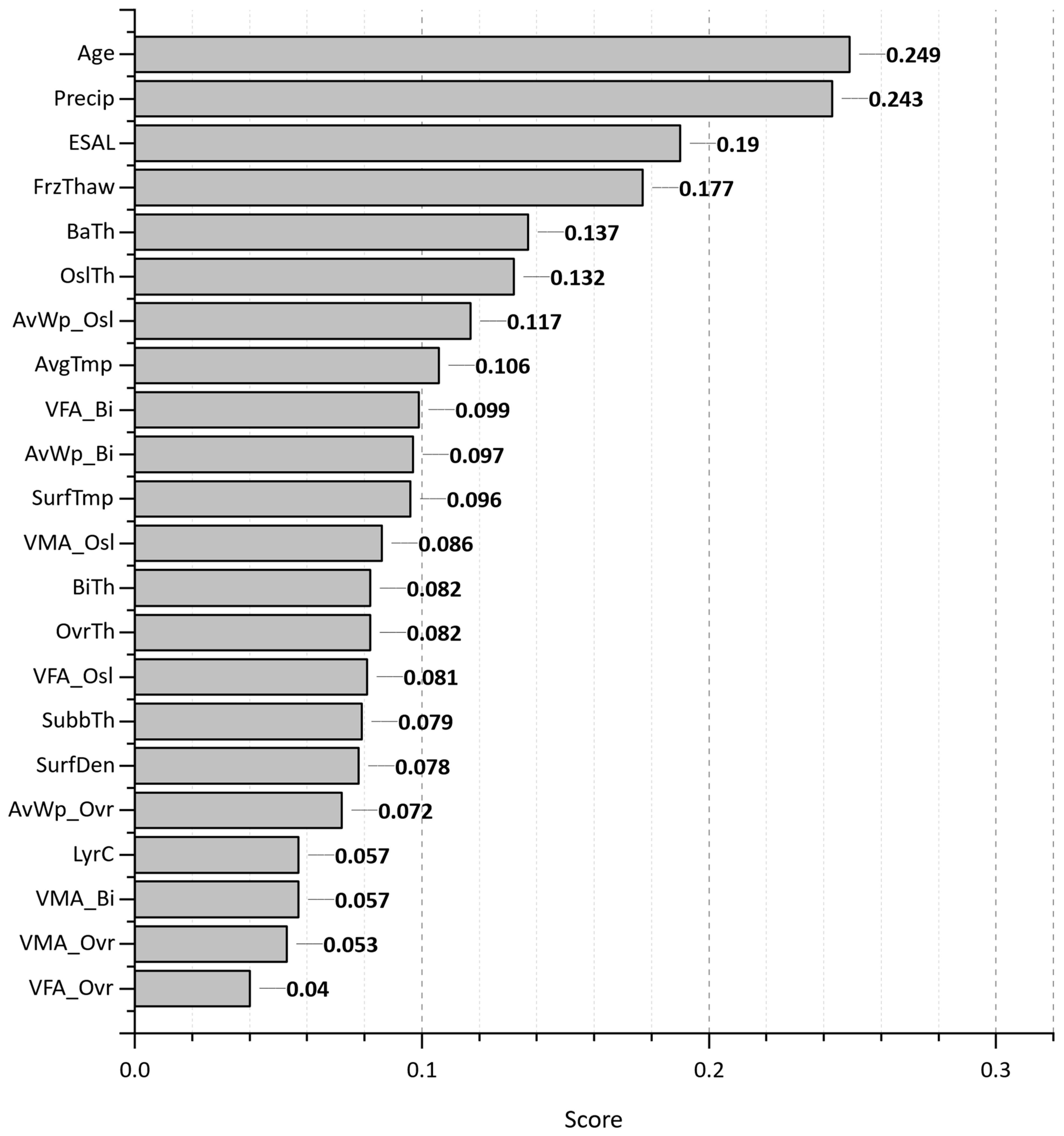
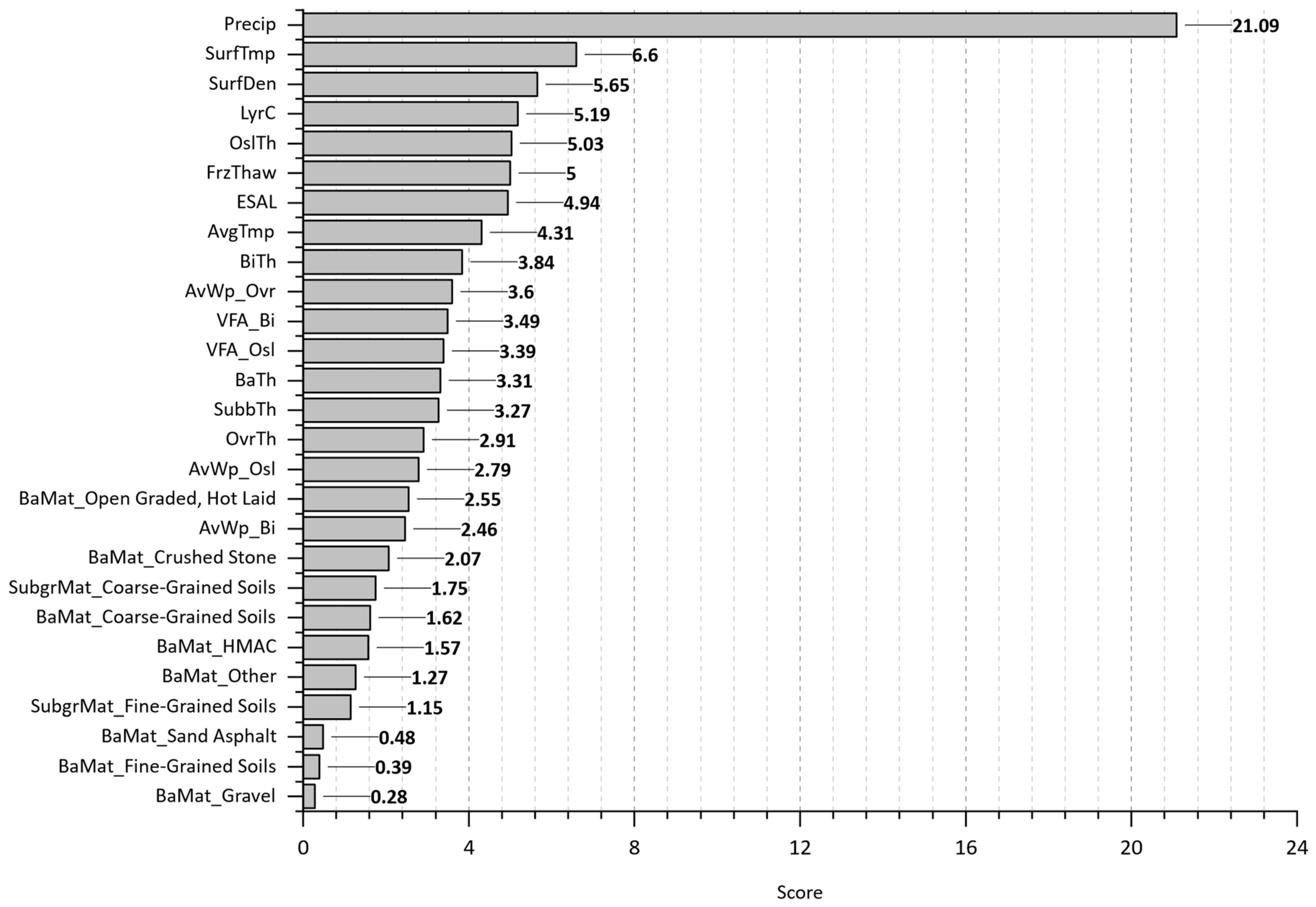
Table 1.
A comparative analysis of AC pavement cracking predictive models.
| Models | Considered Factors | Accuracy | Year | References | ||
|---|---|---|---|---|---|---|
| 1 | Poisson loglinear model | 1. Viscosity of the AC layer. 2. Min and Max mean annual temperature. 3. Average Annual Precipitation. | R2 = 0.47 | 2007 | Ker, H. et al. [39] | |
| 2 | Generalized additive mode | 1. Age. 2. ESAL. 3. Average Annual Precipitation. 4. Average Annual Temperature. 5. Critical tensile strain. 6. Annual freeze–thaw cycle. | R2 = 0.49 | 2007 | Ker, H. et al. [39] | |
| 3 | Multiple regression | 1. Pavement age since overlay. 2. Moisture content of subgrade soil. 3. Climate data. | R2 = 0.88 | 2020 | Radwan et al. [40] | |
| 4 | Machine Learning | 1. Age. 2. ESAL. 3. Average annual precipitation. 4. Average annual temperature. 5. Average annual daily traffic. 6. Average annual Daily Truck Traffic. 7. Annual freeze index. 8. International roughness index. | 9. Total Thickness. 10. Moisture Content. 11. Annual Average Wind Velocity. 12. Climate Zone. 13. Resilient Modulus. 14. Annual Average Humidity. 15. Air Voids. 16. Min and Max Humidity. 17. Marshal stability. | R2 = 0.71 | 2024 | Alnaqbi et al. [41] |
Table 2.
A description of the extracted LTPP features.
| Category | Acronym | Feature | Description | Range|Unit | |
|---|---|---|---|---|---|
| 1 | Pavement Structure and Construction | CN | Construction Number | Changes in pavement structure. | 1–3|- |
| 2 | LyrC | Layer Count | The overall number of layers in a section throughout a construction number. | 3–11|- | |
| 3 | OvrTh | Overlay thickness | The thickness of the overlay layer. | 0–8|Inches | |
| 4 | OslTh | Original surface layer thickness | The thickness of the original surface layer. | 0–7.6|Inches | |
| 5 | BiTh | Binder layer thickness | The thickness of the AC layer below the surface (Binder Course). | 0–13.4|Inches | |
| 6 | BaTh | Base layer thickness | The thickness of the base layer. | 2.5–17|Inches | |
| 7 | SubbTh | Subbase layer thickness | The thickness of the subbase layer. | 0–37.8|Inches | |
| 8 | BaMat | Base layer Material | The type of material used for the base layer. | - | |
| 9 | SubgrMat | Subgrade layer Material | The type of material used for the subgrade layer. | - | |
| 10 | Construction Quality | AvWp | Wheel path air void | Average calculated air voids in the wheel path in the binder, original surface, and overlay layers. | 0–16|% |
| 11 | Den | Density | The density of the top surface layer, e.g., original surface or overlay layers. | 127–149|lb/ft3 | |
| 12 | VFA | Voids Filled Asphalt | The percentage of the total volume of the voids in the compacted aggregate that is filled with asphalt for the binder, original surface, and overlay layers. | 0–94|% | |
| 13 | VMA | Voids Mineral Aggregate | The percentage of the total volume of the voids between the mineral aggregate particles of a compacted asphalt mixture that includes the air voids and the volume of the asphalt binder not absorbed into the aggregate for the binder, original surface, and overlay layers. | 0–30|% | |
| 14 | SurfTmp | Surface Laydown Temperature | Average temperature of the asphalt concrete at lay down for original surface or overlay layers. | 200–340|℉ | |
| 15 | Climate | AvgTmp | Average Ambient Temperature | Average of the daily air temperatures 2 m above the MERRA centroid in between survey dates. | 29–86|℉ |
| 16 | Precip | Precipitation | The cumulative water equivalent of total surface precipitation over a month for each construction number. | 0–344|Inches | |
| 17 | FrzThaw | Freezing Thaw | The cumulative number of days in the month when the maximum air temperature is greater than 0 and minimum air temperature is less than 0 degrees Celsius on the same day. | 0–480|days | |
| 18 | Traffic | ESAL | Equivalent Single Axle Load | Estimated annual equivalent single axle load (ESAL) for vehicle classes 4–13 on LTPP lanes. ESAL values are cumulative traffic loading summary statistics. | 0–12e+6|- |
| 19 | In-service | Service Age | Age | The service age of a given section during one construction number period. | 0–32|Years |
| 20 | WpCrAr | Wheel path Crack per area | The wheel path cracking length divided by the area of the given section. | 0–0.2|ft/ft2 | |
| 21 | AgeCrack | Crack initiation age | Age at which the initial wheel path cracking was observed. | 0.25–20/years |
Table 3.
High-performance computing specification.
| Parameters | Resource |
|---|---|
| CPU | Intel Xeon (R) E5 2670 @ 2.60 GHz, 32 Cores |
| RAM | 32 GB DDR4 2600 MT/s |
| GPU | NVIDIA GeForce GTX 1080 Ti, with 11 GB GDDR5X Memory |
| Disk | Panasas Parallel Storage, Up to 156 TB usable in a RAID-6 configuration |
| NCU/year | 35.50 USD |
Table 4.
Comparing different aspects of machine learning models.
| Attributes | Random Forest | Extremely Randomized Trees | Extreme Gradient Boosting |
|---|---|---|---|
| Learning Method | Ensemble learning | Ensemble learning | Ensemble learning–Gradient boosting algorithm |
| Complexity | Low to medium | Low to medium | Medium to high |
| Interpretability | Medium | Low to medium | Low to medium |
| Scalability | High | High | Medium to high |
| Robust-ness | Medium | Medium | Medium to high |
| Versatility | High | High | High |
| Regression | Uses multiple trees; Average results for Regression | Builds trees using the whole dataset; Randomized thresholds for splits | Sequentially adds trees; Each new tree corrects predecessor errors |
| Optimization Technique | Reducing variance through averaging predictions | Reducing variance through averaging predictions | Gradient boosting with regularization terms |
| Base Learner | Decision Trees | Decision Trees | Decision Trees or Linear Models |
| Handling Missing Data | Imputation or surrogate splits | Internally | Sparsity-aware split finding |
Table 5.
A comparison of different optimization algorithms.
| Features | Bayesian | Grid Search | Randomized Search |
|---|---|---|---|
| Search Type | Probabilistic | Deterministic | Stochastic |
| Accuracy | High | Medium to High | Medium |
| Computation | Fast | Slow | Medium to Fast |
| Strategy | Surrogate model-based (e.g., Gaussian process) | User-defined (applicable to various functions) | User-defined (applicable to various functions) |
| Objective function | Sequential model-based optimization | Full factorial search over specified parameter ranges | Random sampling of parameters from specified distributions |
| Advantages | Can handle noisy data | Systematic exploration of parameter space | Less computationally intensive |
| Disadvantages | Challenging to set priors | Computationally intensive, not scalable with dimensionality | May miss optimal parameters |
Table 6.
A comparative analysis of the most important features for wheel path crack per area (WpCrAr) and crack initiation age (AgeCrack) across three predictive models.
Table 6.
A comparative analysis of the most important features for wheel path crack per area (WpCrAr) and crack initiation age (AgeCrack) across three predictive models.
| Random Forest | Extra Trees | XGBoost | |||
|---|---|---|---|---|---|
| Most Important Features | WpCrAr | 1 | ESAL | LyrC | ESAL |
| 2 | Age | Age | LyrC | ||
| 3 | Precip | Precip | Age | ||
| 4 | FrzThaw | ESAL | Precip | ||
| 5 | OslTh | FrzThaw | OslTh | ||
| AgeCrack | 1 | Precip | Precip | Precip | |
| 2 | VFA_Osl | SurfTmp | ESAL | ||
| 3 | VFA_Bi | SurfDen | VFA_Osl | ||
| 4 | SurfDen | LyrC | AvgTmp | ||
| 5 | ESAL | OslTh | FrzThaw |
Table 7.
Hyperparameter tuning results of randomized search (RS) *, grid search (GS) **, and Bayesian (B ***) optimization methods for the machine learning models.
Table 7.
Hyperparameter tuning results of randomized search (RS) *, grid search (GS) **, and Bayesian (B ***) optimization methods for the machine learning models.
| Random Forest | Extra Trees | XGBoost | |||||||
|---|---|---|---|---|---|---|---|---|---|
| Parameters | RS * | GS ** | B *** | RS | GS | B | RS | GS | B |
| bootstrap | False | False | False | False | False | False | - | - | - |
| max_depth | 30 | 29 | 45 | 26 | 25 | 46 | 17 | 13 | 23 |
| max_features | sqrt | sqrt | log2 | log2 | log2 | sqrt | - | - | - |
| max_leaf_node | None | None | None | None | None | None | - | - | |
| min_samples_leaf | 1 | 1 | 1 | 1 | 1 | 1 | - | - | - |
| min_samples_split | 2 | 3 | 3 | 5 | 4 | 3 | - | - | - |
| n_estimators | 1200 | 1100 | 2000 | 2000 | 1900 | 2000 | 2300 | 1850 | 2700 |
| subsample | - | - | - | - | - | - | 0.8 | 0.7 | 0.75 |
| min_child_weight | - | - | - | - | - | - | 8 | 7 | 7 |
| learning_rate | - | - | - | - | - | - | 0.01 | 0.009 | 0.01 |
| gamma | - | - | - | - | - | - | 1.2 | 0.95 | 0.93 |
| colsample_bytree | - | - | - | - | - | - | 0.85 | 0.8 | 0.85 |
| cross-validation | 5 | 5 | 10 | 5 | 5 | 10 | 5 | 5 | 10 |
| n_iter | 500 | - | 38 | 500 | - | 28 | 500 | - | 30 |
| total fits | 2500 | 400 | 380 | 2500 | 675 | 280 | 2500 | 1500 | 300 |
| time | 7.5 min | 14 min | 18 min | 4.5 min | 10 min | 12 min | 12 min | 35 min | 15 min |
Table 8.
Comparing performance metrics of machine learning models on training and testing datasets for wheel path crack per area (WpCrAr) and crack initiation age (AgeCrack).
Table 8.
Comparing performance metrics of machine learning models on training and testing datasets for wheel path crack per area (WpCrAr) and crack initiation age (AgeCrack).
| XGBoost | Extra Trees | Random Forest | |||||||||
|---|---|---|---|---|---|---|---|---|---|---|---|
| Optimization | Random Search | Grid Search | Bayesian | Random Search | Grid Search | Bayesian | Random Search | Grid Search | Bayesian | ||
| Model | I | II | III | IV | V | VI | VII | VIII | IX | ||
| WpCrAr | Training | R2 | 0.948 | 0.957 | 0.983 | 0.973 | 0.970 | 0.972 | 0.939 | 0.965 | 0.970 |
| MSE | 0.888 | 0.725 | 0.453 | 0.464 | 0.528 | 0.470 | 1.046 | 0.995 | 0.513 | ||
| MAE | 0.472 | 0.427 | 0.352 | 0.296 | 0.319 | 0.296 | 0.587 | 0.456 | 0.315 | ||
| RMSE | 0.942 | 0.851 | 0.673 | 0.681 | 0.727 | 0.686 | 1.022 | 0.997 | 0.716 | ||
| Testing | R2 | 0.753 | 0.761 | 0.791 | 0.749 | 0.747 | 0.751 | 0.725 | 0.756 | 0.747 | |
| MSE | 4.250 | 4.131 | 3.862 | 4.302 | 4.442 | 4.302 | 4.820 | 4.177 | 4.345 | ||
| MAE | 1.131 | 1.104 | 1.071 | 1.088 | 1.102 | 1.089 | 1.264 | 1.115 | 1.099 | ||
| RMSE | 2.061 | 2.032 | 1.965 | 2.074 | 2.107 | 2.074 | 2.195 | 2.044 | 2.084 | ||
| AgeCrack | Training | R2 | 0.952 | 0.961 | 0.987 | 0.993 | 0.990 | 0.992 | 0.968 | 0.994 | 0.999 |
| MSE | 0.373 | 0.270 | 0.117 | 0.152 | 0.190 | 0.156 | 0.535 | 0.484 | 0.002 | ||
| MAE | 0.293 | 0.248 | 0.173 | 0.195 | 0.218 | 0.195 | 0.291 | 0.200 | 0.019 | ||
| RMSE | 0.611 | 0.520 | 0.342 | 0.390 | 0.436 | 0.395 | 0.360 | 0.335 | 0.054 | ||
| Testing | R2 | 0.883 | 0.891 | 0.921 | 0.902 | 0.905 | 0.909 | 0.865 | 0.896 | 0.907 | |
| MSE | 1.855 | 1.777 | 1.603 | 1.839 | 1.979 | 1.839 | 2.190 | 1.766 | 1.874 | ||
| MAE | 0.807 | 0.780 | 0.747 | 0.790 | 0.804 | 0.791 | 0.930 | 0.781 | 0.765 | ||
| RMSE | 1.362 | 1.333 | 1.266 | 1.356 | 1.389 | 1.356 | 1.480 | 1.329 | 1.369 | ||
Disclaimer/Publisher’s Note: The statements, opinions and data contained in all publications are solely those of the individual author(s) and contributor(s) and not of MDPI and/or the editor(s). MDPI and/or the editor(s) disclaim responsibility for any injury to people or property resulting from any ideas, methods, instructions or products referred to in the content. |
© 2024 by the authors. Licensee MDPI, Basel, Switzerland. This article is an open access article distributed under the terms and conditions of the Creative Commons Attribution (CC BY) license (https://creativecommons.org/licenses/by/4.0/).
Share and Cite
MDPI and ACS Style
Taheri, A.; Sobanjo, J. Ensemble Learning Approach for Developing Performance Models of Flexible Pavement. Infrastructures 2024, 9, 78. https://doi.org/10.3390/infrastructures9050078
AMA Style
Taheri A, Sobanjo J. Ensemble Learning Approach for Developing Performance Models of Flexible Pavement. Infrastructures. 2024; 9(5):78. https://doi.org/10.3390/infrastructures9050078
Chicago/Turabian StyleTaheri, Ali, and John Sobanjo. 2024. "Ensemble Learning Approach for Developing Performance Models of Flexible Pavement" Infrastructures 9, no. 5: 78. https://doi.org/10.3390/infrastructures9050078