
Major and Minor Contributions to X-ray Characteristic Lines in the Framework of the Boltzmann Transport Equation


Laboratory of Montecuccolino-DIN, Alma Mater Studiorum University of Bologna, via dei Colli 16, 40136 Bologna, Italy
*
Author to whom correspondence should be addressed.
Quantum Beam Sci. 2022, 6(2), 20; https://doi.org/10.3390/qubs6020020
Submission received: 30 March 2022
/
Revised: 29 April 2022
/
Accepted: 6 May 2022
/
Published: 19 May 2022
(This article belongs to the Special Issue X Rays: Physics and Applications)
Abstract
:The emission of characteristic lines after X-ray excitation is usually explained as the consequence of two independent and consecutive physical processes: the photoelectric ionization produced by incoming photons and the successive spontaneous atomic relaxation. However, the photoelectric effect is not the only ionization mechanism driven by incoming photons. It has been recently shown that Compton ionization is another possible process that contributes not negligibly to the ionization of the L and M shells. In addition, the secondary electrons from these two interactions, photoelectric and Compton, are also able to ionize the atom by means of so-called impact ionization. Such a contribution has been recently described, showing that it can be relevant in cases of monochromatic excitation for certain lines and elements. A third mechanism of line modification is the so-called self-enhancement produced by absorption of the tail of Lorentzian distribution of the characteristic line, which mainly modifies the shape of the lines but also produces an intensity increase. The four effects contribute to the formation of the characteristic line and must be considered to obtain a precise picture in terms of the shell and the element. This work furnishes a review of these contributions and their formal theoretical descriptions. It gives a complete picture of the photon kernel, describing the emission of characteristic X-rays comprising the main photoelectric contribution and the three effects of lower extent. All four contributions to the characteristic X-ray line must be followed along successive photon interactions to describe multiple scattering using the Boltzmann transport equation for photons.
1. Introduction
It is universally accepted that X-ray characteristic lines are produced by the dominant mechanism represented by the spontaneous relaxation of the atom following ionization due to the photoelectric effect. Thus, the energy of the line is determined by the energy difference between the energy levels involved in the electronic transition, giving origin to the term “characteristic line”. Since the photoelectric effect is a well-understood phenomenon, it is possible to fully determine the line intensity in terms of atomic parameters such as the line emission probability, which depends on the line fraction and the fluorescence yield, the atomic abundance given by the element weight fraction, the specimen density, and the photoelectric effect probability of the ionized atomic shell. The precision in the calculation of the intensity depends on the precision with which the mentioned atomic parameters are known. These atomic parameters are not easy to determine individually since they are extracted from measurements of characteristic lines and appear always in a combination. Many years of measurements and calculations from several authors have led to the acquisition of complete databases of atomic parameters that appear quite reliable. By computing line intensities with these databases, several authors have found differences among the measured values [1,2,3,4,5,6,7,8,9,10]. These differences can be attributed to other processes of minor extent if compared with the photoelectric ionization. Three of these processes have been studied in recent publications and are far from being considered negligible in certain favorable experimental conditions. They are intensity contribution due to Compton ionization; intensity enhancement due to the inner-shell impact ionization of secondary electrons (released by both ionization mechanisms: photoelectric and Compton); and intensity modification due to self-absorption of the Lorentzian tail in the photoelectric absorption edge. This paper collects the known information on these processes. Their description in a unique source makes it possible to compare them by stressing the conditions under which they become more relevant. The comparison will make clear that each of the three additional processes contributes to intensity, thereby explaining the difference between the intensity computed only with the dominant process of photoelectric ionization and the experimental one.
2. Theory
2.1. The Boltzmann Scalar Transport Equation
There exist different degrees of approximation to describe the diffusion of photons using the Boltzmann transport equation. The simpler is the scalar model [11], which considers photons whose (average) polarization states are not modified, and therefore, it is not possible to describe the effects of their polarization states. This model is based on the balance between the number of photons of given energy and direction entering and leaving the considered volume element. This balance can be formulated for conditions where the X-ray source is constant in time (steady-state) and, therefore, also the flux of the photons in the medium.
If we consider a point and an infinitesimal right cylinder with a base area centered at at height whose lateral surface is parallel to the direction , the flux is defined as the number of photons with energy between and , and with direction between and , which cross a unit area of the base of the infinitesimal cylinder per unit time. The scalar integral-differential Boltzmann transport equation, for a simple model of backscattering from an infinitely thick target, is defined as:
where and are the unit vectors defining the propagation direction of the photons before and after a generic interaction, respectively; and are the energy before and after the interaction, respectively; denotes the directional cosine ; is the differential of the solid angle in the direction of the unitary vector; is the total mass attenuation coefficient; is the unitary step Heaviside function; is the single-process kernel of photon scattering in from ; and represents an external source of photons. Although this equation is one-dimensional, it contains the full phase-space information about the incident, as well as take-off directions and the energy of the photons.
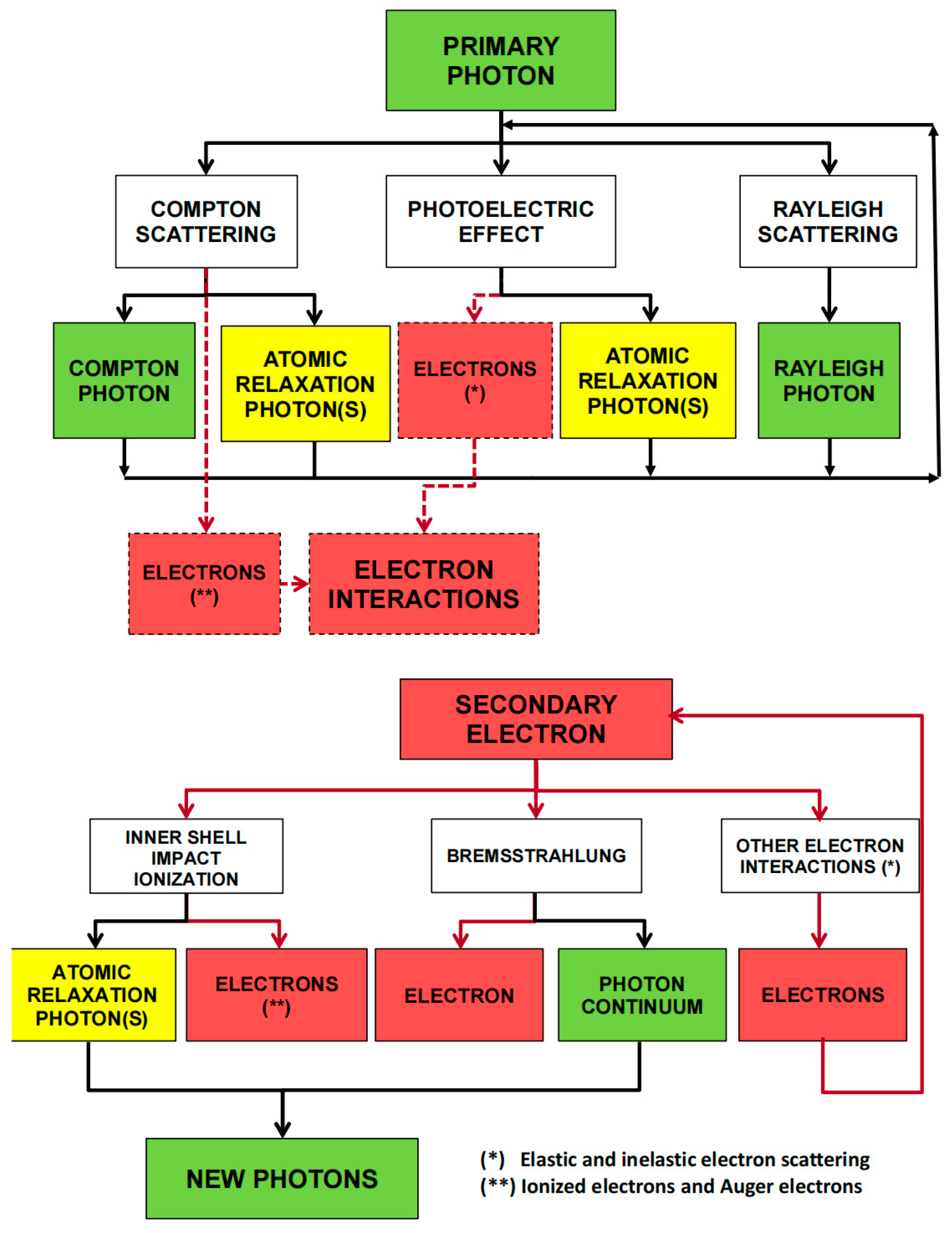
As can be seen in Figure 1, secondary electrons may produce photons through two interaction mechanisms: bremsstrahlung (which produces a continuous photon energy spectrum) and inner-shell impact ionization (ISII) (an inelastic collision which ionizes the interacting atom, causing a vacancy in the atomic shell that is filled through a relaxation process). These two electron radiative contributions can be introduced as additional kernel terms to the photon Boltzmann transport model if they are computed externally. In this way, the new equation is able to also comprise the contribution from the secondary electrons to the photon field. By using this approach, the Boltzmann equation can be rewritten as:
where denotes now the single-process photon-to-photon interaction kernel and is the single-process electron-to-photon interaction kernel. The contribution from the secondary electrons is contained in the new electron-to-photon interaction kernels. As it can be seen from Equation (2), these corrective kernels contribute to the photon field in a similar way to that performed by the scattering coefficient containing the single-process photon-to-photon interaction kernels.
The influence of X-ray interactions in the transport process is considered in Equation (2) through the total mass attenuation coefficient and the single-process kernels. These two magnitudes are directly related to the interaction cross-section , which represents, for a generic photon interaction , the probability density function for photons having direction and energy .
The total mass attenuation coefficient is defined as the probability that photons with energy give rise to any one of the X-ray possible interactions and, in the considered model, is expressed as:
In terms of the mass attenuation, the coefficients for the single interactions are for Rayleigh scattering, for Compton scattering, and for the photoelectric effect.
The single-process kernel is defined per unit path through the medium and per unit of solid angle and energy of scattered photons as the probability density function that photons from scatter in . The single-process kernel for the generic interaction can be expressed as the double differential cross-section of the interaction:
The scattering cross-section for the process can be obtained from the following relation:
In what follows, we give a detailed description of the interaction kernels for the dominating interactions that play a direct role in the production of XRF characteristic lines. Three of them are due to physical processes that correspond to single terms in the Boltzmann transport equation. They are the atomic relaxation following the photoelectric effect (which represents the major contribution) and the atomic relaxations following Compton ionization and inner-shell impact ionization, which represent two minor contributions. All these contributions are represented as yellow boxes in the interaction scheme of Figure 1 and are described in the following sections. A third minor contribution is from self-enhancement absorption, which needs a separated description because is not associated directly to an interaction kernel.
2.2. X-ray Line Intensity Due to Photoelectric Ionization
The classical process that describes the emission of characteristic X-ray lines is photoelectric ionization. In this important interaction, a photon is absorbed by the atom, which ionizes it and releases an electron with energy equal to the difference between the energy of the absorbed photon and the binding energy of the ionized shell of the target atom . The vacancy left by this interaction is spontaneously filled by an electron transition from a higher energy level, giving rise to a process called atomic relaxation. The de-excitation energy is carried off with the emission of a characteristic photon or Auger electrons. Since the two consecutive processes are almost simultaneous, the combined process (absorption plus relaxation) may be considered as a sort of inelastic “scattering” interaction.
The interaction kernel for the emission of a characteristic line of energy from a pure element target because of photoelectric absorption of photons with energy is given by [12]:
The kernel independence on and the normalization factor reflect the isotropy of the emitted X-rays. The Heaviside function allows the photoelectric interaction only for energy values of the primary photon greater than the threshold of the absorption edge energy for the considered line The emitted line is assumed to be monochromatic with the energy value , as expressed by the delta function in Equation (6). represents the X-ray fluorescence (XRF) emission probability density of a line that belongs to a series, and it is given by the following relation:
In Equation (7), represents the photoelectric attenuation coefficient (in cm−1) of the emitter element ; is the probability of photon interaction with the shell (see Appendix A); is the probability of X-ray emission as a consequence of relaxation to the same shell; and, finally, is the emission probability of the characteristic line with energy inside its own spectral series. The complete kernel describing all the characteristic lines emitted by element is obtained by summing the of the element:
An alternative to the shell probabilities in Equation (7) is the use of the shell mass attenuation coefficient . To this end, the photoelectric total atomic cross-section and partial cross-sections for the photoionization of the K, L, M and N shells for all elements with Z from 1 to 99 in the energy range from 50 eV to 1 TeV are reported in the EPDL97 database [13].
2.3. XRF Contribution from Compton Ionization of Single Shells
Even if the impulse approximation (IA) allows the computation of the Compton cross-section for each shell of the considered element in a rather simple way (by the use of the Compton profile), it is well-known that this description fails to evaluate the Compton cross-section when the energy of the primary photon moves closer to the binding energies of the atomic shells. Otherwise, the Waller–Hartree (WH) approximation gives a good description of the Compton cross-section, even in energy ranges close to the binding energies of the considered element, but precludes the possibility to depict the contribution of each single shell to the total Compton cross-section. To overcome possible inaccuracies due to the IA approximation limits, a single-shell Compton cross-section is computed through the following expression:
Here, and are, respectively, the total Compton cross-sections in the WH and the IA approximations, giving the following expressions:
The WH scattering function in Equation (14) is obtained by interpolating the tables by J.H. Hubbell [13].
As shown by Fernandez et al. [14], Compton scattering is an ionization process that, in some cases, gives rise to a non-negligible atomic relaxation contribution. The XRF contribution due to Compton ionization becomes bigger for external shells such as the L and M shells.
The contribution due to Compton scattering can be added directly into the photoelectric cross-section shown in Equation (8) as a corrective term for each considered line , defined as:
which obtains the new characteristic line kernel correction
where denotes the energy of the Compton peak.
This kernel correction allows the addition to the Boltzmann model of the atomic relaxation contribution due to Compton ionization process for each shell from K to M5.
2.4. XRF Contribution from Inner-Shell Impact Ionization by Secondary Electrons
The scheme in Figure 1 illustrates the coupling mechanism between photons and electrons. In general, the codes that describe photon transport neglect electron contributions and focus only on the higher block of the scheme. The reason is that the solution for the coupled problem is time-consuming and difficult to describe, even with Monte Carlo codes, because the electrons interact continuously with the medium and, therefore, the number of electron collisions is always very high. This contribution has been evaluated recently by Fernandez et al. [15,16] as a corrective term to be included in photon transport codes with the help of the Monte Carlo code PENELOPE.
The code PENELOPE (coupled electron–photon Monte Carlo) [17] was used to study the effect of secondary electrons on photon transport. An ad-hoc code KERNEL was developed to simulate a forced first collision at the origin of coordinates driven by a point source of monochromatic photons. The physics of the interaction were described using the PENELOPE subroutine library. All the secondary electrons were followed along their multiple scattering until their energies became lower than a predefined threshold value. All the photons produced by the electrons at every stage were accumulated. Polarization was not considered at that time.
The simulated process is summarized by the following points:
- A photon with energy E0 situated in an infinite medium came along the z-axis and hit an atom in the origin of the reference frame; in the range of interest (the program was not limited to that), 1–100 keV, it could interact through three different processes: photoelectric effect, coherent (Rayleigh) scattering, and incoherent (Compton) scattering. The first and the third processes involved the production of secondary electrons. These particles were stored in the secondary stack if their energy exceeded the absorption limit. PENELOPE also simulated pair production, but the threshold energy for this kind of interaction was of the order of 1 MeV and, therefore, was not comprised of lower energies;
- After the interaction, the secondary stack was checked in order to verify the presence of particles; if it was found empty, the photon suffered a Rayleigh interaction, and the code went back to point 1, starting a new shower. Otherwise, it proceeded to point 3;
- The secondary stack could contain electrons, positrons, or photons. The program started to simulate the slowing process for electrons and positrons until their energy fell to the absorption edge. If there was a photon stored in the secondary stack, the program skipped to the following particle. The transport of secondary photons was ignored. Charged particle interactions involved the production of other charged particles and photons: the first were stored in the secondary stack; the photon properties were scored in order to obtain angular, energy, and spatial distributions. These distributions were tallied for bremsstrahlung emission and inner-shell impact ionization;
- The simulation of the shower continued until the secondary stack was empty and all the charged particles stored in it completed their ‘lives’. At this point, the shower was completed, and the kernel started the generation of a new one (point 1).
The electron contribution to photon transport is due to two types of interactions: (a) Bremsstrahlung, which contributes a continuous distribution; and (b) inner-shell impact ionization, which modifies the intensity of the characteristic lines.
Both contributions have been studied recently [14,15,16]. For the XRF contribution, we will focus only on inner-shell impact ionization, which is the only one capable to ionize the atom. The angular distribution of characteristic photons produced by atomic relaxation following inner-shell impact ionization can be considered isotropic. The spatial distribution of the photons can be ignored, and the source of characteristic photons can be safely represented as point one. To quantify the correction in terms of energy, calculations are performed for all the lines of the elements Z = 11–92 in the energy range of 1–150 keV. Since electrons lose their energy more efficiently in the low energy range, the computed contribution is always higher for low energy lines.
To avoid database differences between PENELOPE and other transport codes, the electron correction is computed in units of the photon photoelectric contribution :
with
It is worth noting that the condition for impact ionization is that the energy of the hitting electrons reaches the extent of the binding energy of the new electron to remove. The threshold condition in Equation (14) is related to the source photons and not to the electrons. To parameterize the correction for a generic energy, the whole interval is divided into five energy regions delimited by the K, L1, L2, and L3 absorption edges. The best fit of the energy correction at each interval is computed using four coefficients, as follows:
2.5. Characteristic Lines Kernel Comprising the Three Interaction Terms Computed so Far
As shown in the previous sections, there are two minor ionization processes that, in some cases, give rise to a non-negligible atomic relaxation contribution. The contributions due to Compton scattering ionization and inner-shell impact ionization can be added directly into the photoelectric cross-section ionization for each considered line , obtaining the following corrected kernel for characteristic lines:
that uses the following modified emission probability:
This new kernel expression allows the addition to the Boltzmann model of the atomic relaxation contribution due to the Compton ionization process for each shell from K to M5.
2.6. Contribution of Self-Enhancement
Each one of the three contributions considered above is an independent physical interaction and is shown with a yellow box in Figure 1. There exists a fourth contribution that is due to the effect of Lorentzian broadening of the characteristic line, which overlaps (and is absorbed by) the absorption edge, as shown in Figure 2. This kind of absorption becomes clear by comparison with the Dirac delta approximation, which usually simplifies the description of the characteristic lines.
2.6.1. Dirac Approximation
In a first approximation, characteristic lines are assumed to be perfectly monochromatic, neglecting their natural widths. Therefore, for a single characteristic line of energy , the emission kernel given by Equation (17) is a delta-one and is denoted as: .
2.6.2. Lorentzian Shape
A better description of the line shape assumes a Lorentzian distribution with as the HWHM (the FWHM being the natural width of the lines) [18]. Thus, the total photoelectric kernel becomes:
with the Lorentzian function defined as:
The term in Equation (19) expresses the physical impossibility of a tail contribution exceeding the excitation energy E’. As the tail of the Lorentzian shape exceeds and overlaps the K edge, it is strongly absorbed in the specimen material. Then, it is possible to consider the effect of such an absorption to refine the description of the intensity.
2.6.3. Solution of the Transport Equation with the Lorentzian Kernel
To find the contribution of self-absorption, it is possible to follow the steps described in [19]. A first approximation of the self-enhancement contribution can be estimated by using the first-order solution of the Boltzmann transport equation. The first-order analytical solution of the transport equation for the interactions in Equation (19) gives the extent of the intensity of the characteristic lines emitted after excitation with a photon beam. For the sake of simplicity, it is considered a monochromatic excitation of energy . The first-order flux for a source of photons cm−2 s−1 is given by:
Here, and are the cosines of the incident and outgoing directions, respectively; is the mass attenuation coefficient at the energy ; and is the mass attenuation coefficient at .
The first-order integrated intensity is defined as:
followed by:
For the single line of energy , the intensity is as follows:
To obtain the primary intensity, it is necessary to compute the integral in Equation (23). Analogously, it is possible to obtain expressions for the secondary and tertiary intensities [12].
Let us consider the effect of the K-edge absorption to obtain a description of the modified intensity. The tail absorption starts a self-enhancement process, i.e., a secondary enhancement produced by the same type of atom that emitted the absorbed line. The self-enhancement term for a single line can be computed by using the second-order flux described in [12], as follows.
In the first approximation, the total intensity for a single Lorentzian line absorbed by the K edge comprising the enhancement term is:
where
Equation (25) gives the enhancement at produced by a monochromatic line j centered at the edge energy . Every single term is generated by the fractional tail intensity , according to the following:
The total enhancement is obtained by summing the contributions from all the characteristic lines in the series crossing the K edge. Equation (24) can be rewritten as:
Equation (27) contains the self-enhancement contributed by tail absorption in the first order. Since the contributed intensity always has the same energy, this correction can be replicated iteratively by considering absorptions of the second-order, third-order, and so on, leading to the following closed expression valid only for K lines of pure elements:
The maximum of the Lorentzian line centered at is expected to be higher because of the self-enhancement term between parenthesis, which is greater than 1. The overall intensity obtained by integration is slightly reduced because of high energy truncation due to the attenuation term.
2.6.4. Characteristic Lines Kernel Comprising all Corrections (Interactions Plus Self-Enhancement)
In what follows, the kernel is shown for the characteristic lines comprising all the mentioned effects: the major contribution from atomic relaxation following photoelectric ionization, the two relaxation contributions (the first from Compton ionization and the second from electron impact ionization), and, finally, the contribution from self-enhancement due to Lorentzian tail absorption.
Equation (29) describes the delta kernel for the complete set of n characteristic lines. For the single line centered at the energy , the kernel is:
Both the ISII and the Compton ionization contributions are positive and, therefore, contribute to increasing the height of the line. The self-enhancement correction is larger than 1 and, therefore, increases the height of the line. However, because of the truncation due to high energy tail attenuation, the integrated area of the line may decrease in certain situations. It is worth noting that this small decrease in the area is not connected to the line height. This different and contrasting behavior of the area and the height of the line is worth consideration with more detail since normal practice is to assume the peak area as proportional to the line height and width (for a Gaussian peak, the area is 1.0645 × height × FWHM).
X-ray spectroscopists use estimating the peak area from the line height and width. In this case, it is better to consider a slightly different kernel (omitting truncation):
that is larger than the uncorrected one. The kernel defined by Equation (31) appears more adequate for use in experimental spectroscopy because it gives the total area under the line that incorporates all physical contributions to the peak.
3. Results and Discussion
The major contribution to X-ray characteristic lines is due to atomic relaxation following photoelectric ionization and is described by kernel Equation (9). The calculation method shown in this paper uses the shell probabilities described in Appendix A to obtain the shell mass attenuation coefficients from the total one. It requires knowledge of the total mass attenuation coefficient of the element, the Koster–Cronig coefficients, the fluorescence yields for the shells, and the relative intensities of the lines in their own series. These parameters can be obtained individually from sparse bibliographical sources [20,21,22,23] or from atomic data compilations such as those of Elam [24], Schoonjans [25], or Cullen [13]. An alternative computation method uses single-shell attenuation coefficients, such as those in the EPDL97 database [26] or those computed recently by Sabbatucci and Salvat [27], instead of shell probabilities.
The previous section describes the three different corrective contributions that deserved attention in this article. They are discussed below.
- Atomic relaxation from Compton ionization: The characteristic line intensity correction due to Compton ionization was computed for the shells K, L, and M of elements with Z = 11–92 [14]. The energy to reach a given extent of correction (1, 5, 10, 20, 50, or 100%) as a function of Z was computed for the shells K, L1–L3, and M1–M5. It was demonstrated that the contribution from single-shell Compton ionization plays a role in the description of radiation fields in X-ray spectrometry, especially for the L and M shells (Figure 3 and Figure 4).
- Atomic relaxation from electron impact ionization: The inner-shell impact ionization correction was studied in terms of spatial, angular, and energy distribution. It was shown that the correction was point-wise and isotropic. The energy dependence of the correction was parameterized using 20 parameters (five energy regions of four parameters each) for all lines of elements Z = 1–92 in the range of 1–150 keV. It was shown that the absolute correction to the line intensity was concentrated in a limited energy interval, making the correction more important for monochromatic excitation lying in such an interval than for polychromatic excitation (Figure 5).
Figure 3.
Values of the energy in keV as a function of the atomic number Z, for which σL3/τL3 became larger than 1%, 5%, 10%, 20%, 50%, and 100%. These values were computed using the EPDL97 database. This shows the extent of the correction for the Mo lines of L3, α1, and α2 when the exciting source was around 50 keV.

Figure 4.
Values of the energy in keV as a function of the atomic number Z, for which the ratio σM5/τM5 became larger than 1%, 5%, 10%, 20%, 50%, and 100%. These values were computed using the EPDL97 database. This shows the extent of the correction for the W lines of M5, α1, and α2 when the exciting source was around 50 keV.

Figure 5.
Top panel: and for the line Na as a function of the excitation energy in keV. Lower panel: The absolute correction was relevant within a restricted interval. The maximum extent of the correction occurred at 5 keV and represented 4.63% of the uncorrected line.
Figure 5.
Top panel: and for the line Na as a function of the excitation energy in keV. Lower panel: The absolute correction was relevant within a restricted interval. The maximum extent of the correction occurred at 5 keV and represented 4.63% of the uncorrected line.

- 3.
- Self-enhancement contribution: This was computed analytically for K lines. It describes what happens with the line intensity when the Lorentzian tail crosses the edge, i.e., the energy of the emitted photon is high enough to produce another vacancy and, therefore, a self-enhancement effect. Figure 6 illustrates the effect for elements from Na to U. For the edges L and M and for mixtures of elements, it was necessary to use other techniques. Since the high energy tail decreased asymptotically, it required refined variance reduction techniques to be used in MC codes. The slow asymptotic decrease of the Lorentzian distribution introduced a further complication to describe multiple scattering with reasonable statistics. A deterministic method based on the energy (wavelength) discretization of the Lorentzian distribution was used with good results (for details see [28]). Calculations on multicomponent samples showed that the multiple scattering terms produced asymmetric contributions modifying the shape of the line (Figure 7).
4. Conclusions
The traditional description of X-ray characteristic lines assumes that they are a consequence of inner-shell photoelectric ionization followed by atomic relaxation. In this article, we showed that this is not the only process occurring in the atom and that there are other processes that contribute to changing the line height and shape. Considering only the major contribution due to photoelectric ionization introduces a systematic error to the line intensity evaluation, which obscures the comparison between experimental intensities and theoretical probabilities. The error increases with the number of minor contributions neglected. For the atomic parameters that are determined indirectly from measurements of intensity, the error of the expected intensity might propagate in their determination. The atomic parameters more affected by an incorrect estimation of the intensity are both the line probabilities and the fluorescence yields.
This work collected and summarized three minor corrections that can be considered to improve the description of X-ray characteristic lines. Complete kernels were given for the corrections in order to be used in MC and deterministic codes of photon transport.
The single corrective contributions analyzed in this article are summarized in Table 1 with mention of the physical mechanism originating them, the specific and distinctive properties of each contribution, and the lines more influenced.
The dominant effect is, of course, the inner-shell photoelectric ionization initiated by the primary source photons.
Two additional ionization processes increase the height of the line. The first one is due to the impact of the secondary electrons released by both the photoelectric effect and Compton scattering. This process may influence the height of certain low-energy K and L lines when adequately excited with monochromatic sources. The example in Figure 5 shows an increase larger than 4% for a certain energy. Simulations for the main lines of all the elements with Z = 11–92 showed that the correction always presented a maximum for monochromatic energy. This effect was less apparent for polychromatic excitation because it was averaged within the energy interval of the excitation source spectrum. The second minor contribution is due to Compton ionization. It is negligible for the K lines of most of the elements. It modifies preferentially the L and M lines and requires an X-ray source of medium-high energy. Figure 3 shows a variation of 5–10% for the L lines of Mo excited with 50 keV X-rays. Analogously, Figure 4 shows that the variation could reach 10–20% for the M lines of W for a source distribution centered at 50 keV. It is worth noting that this process might be influenced by the polarization of the primary beam. This influence will be described in a future article. Both contributions are positive and, therefore, contribute to increasing both the height and the area of the line.
The third minor contribution is of a different nature than the ones described above. It is produced by a self-enhancement mechanism due to photoelectric absorption of the higher energy Lorentzian tails of the lines. It is a second-order effect and is more important for broader lines, such as certain L or M lines. As shown for K lines, the contribution had a different effect on the height and the area of the line. The height increased because the contribution was positive, but conversely, the area decreased because of the effect of the attenuation of the tail. The attenuation on the high-energy side had the effect of changing the shape of the line because of the cut-off. The asymmetry produced by this effect became more important in case of multiple scattering and, therefore, may be larger for lines measured from thick specimens.
The three minor effects described here increase the height of the characteristic line; therefore, they should be considered in order to obtain a better agreement between experiment and theory. This can contribute also to improving the precision of the atomic parameters that require an estimation of line intensity to be determined.
A comparison between measured intensities and calculations comprising these effects is foreseeable in the future. The study should be performed by exploiting the experimental conditions capable of maximizing some of the minor contributions.
Funding
This research received no external funding.
Data Availability Statement
Not applicable.
Conflicts of Interest
The authors declare no conflict of interest.
Appendix A. Relative Shell Probabilities for the Photoelectric Effect
The probability of interaction with the shells of the atom is a function of E’, the energy of the photon. For Z > 10, the ionization of the K shell may produce characteristic emission above 1 keV. The probability of ejecting an electron (i.e., creating a vacancy) from the K shell has the constant value of
where is the edge-jump, i.e., the ratio of the photoelectric cross-sections at the top and bottom of the K edge [29].
For Z > 28, we must also consider L shells. According to [20], the probability of having a vacancy in the shells L1, L2, or L3, respectively, can be written as:
where represents the corresponding edge-jump for the shells L1, L2, and L3, and is the probability for the occurrence of a Coster–Kronig radiationless transition from La Lb [22,23,30].
For Z > 53, we must also consider M shells, considering and . The probability of having a vacancy in the shells M1, M2, or M3, respectively, can be written as:
For the shell M4, it is convenient to write the contribution of each of the other M shells separately:
The total probability of an event in the shell M4 is the sum of the factors above multiplied by the probability of not interacting with the K- and L- shells.
For the shell M5, it is convenient to write the contribution of each of the other M shells separately:
The total probability of an event in the shell M5 is the sum of the factors above multiplied by the probability of not interacting with the K- and L- shells.
If we define , the probability of outer-shell events is:
It is possible to distinguish 10 energy regions, as shown in Table A1. The shell probabilities and the values are summarized in the Table A2 and Table A3.
The atomic parameters involved in these computations, called “fundamental parameters”, are permanently checked, and updated by a group of experts in the framework of the International Initiative of Fundamental Parameters (IIFP) [31]. The initiative is supported by prestigious European, American, and Japanese academic and metrological institutions and counts with the support of important manufacturers of spectrometers. Detailed information about the objectives, the involved institutions, and the companies can be found in the last updated roadmap of the IIFP, published in 2017 [32].

Table A1.
The same Formulas (A1)–(A10) apply to all these regions by addressing these comments.
| Energy Region | Energy Interval | Comments |
|---|---|---|
| 1 | For this region, all the formulas from (A1) to (A10) are valid. | |
| 2 | The energy is not high enough to create a vacancy in the K shell. Therefore, the probability of ejecting an electron from the K shell is always 0: and . With these assumptions, all the previous formulas for L and M shells are still valid. | |
| 3 | The energy is not high enough to create a vacancy in the shells K and L1. Therefore, and . With these assumptions, all the previous formulas for L- and M- shells are still valid. | |
| 4 | The energy is not high enough to create a vacancy in the shells K, L1, and L2. Therefore, , and . | |
| 5 | The energy is not high enough to create a vacancy in the K- and L- shells. Therefore, , , , and . | |
| 6 | The energy is not high enough to create a vacancy in the K-, L-, and M1 shells. Therefore, , , , , and . | |
| 7 | The energy is not high enough to create a vacancy in the K-, L-, M1, and M2 shells. Therefore, , , , , , and . | |
| 8 | The energy is not high enough to create a vacancy in the K-, L-, M1, M2, and M3 shells. Therefore, , , , , , , and . | |
| 9 | The energy is not high enough to create a vacancy in the K, L, M1, M2, M3, and M4 shells. Therefore, , , , , , , , and . | |
| 10 | The interaction is possible only with the outer shells: . All other probabilities are 0. |
Table A2.
Single-shell probabilities of interaction according to the excitation energy. The probabilities are always computed with the Formulas (A1)–(A10).
Table A2.
Single-shell probabilities of interaction according to the excitation energy. The probabilities are always computed with the Formulas (A1)–(A10).
| X-ray Emission Probability by Shell | |||||||||||
|---|---|---|---|---|---|---|---|---|---|---|---|
| Energy Region | Energy Interval | K | L1 | L2 | L3 | M1 | M2 | M3 | M4 | M5 | Outer |
| 1 | |||||||||||
| 2 | 0 | ||||||||||
| 3 | 0 | 0 | |||||||||
| 4 | 0 | 0 | 0 | ||||||||
| 5 | 0 | 0 | 0 | 0 | |||||||
| 6 | 0 | 0 | 0 | 0 | 0 | ||||||
| 7 | 0 | 0 | 0 | 0 | 0 | 0 | |||||
| 8 | 0 | 0 | 0 | 0 | 0 | 0 | 0 | ||||
| 9 | 0 | 0 | 0 | 0 | 0 | 0 | 0 | 0 | |||
| 10 | 0 | 0 | 0 | 0 | 0 | 0 | 0 | 0 | 0 | 1 | |
| Elements Involved | Z > 10 | Z > 28 | Z > 53 | ||||||||
Table A3.
Single-shell probabilities are computed by replacing the values shown here in Formulas (A1)–(A10).
Table A3.
Single-shell probabilities are computed by replacing the values shown here in Formulas (A1)–(A10).
| by Shell | ||||||||||
|---|---|---|---|---|---|---|---|---|---|---|
| Energy Region | Energy Interval | K | L1 | L2 | L3 | M1 | M2 | M3 | M4 | M5 |
| 1 | ||||||||||
| 2 | 1 | |||||||||
| 3 | 1 | 1 | ||||||||
| 4 | 1 | 1 | 1 | |||||||
| 5 | 1 | 1 | 1 | 1 | ||||||
| 6 | 1 | 1 | 1 | 1 | 1 | |||||
| 7 | 1 | 1 | 1 | 1 | 1 | 1 | ||||
| 8 | 1 | 1 | 1 | 1 | 1 | 1 | 1 | |||
| 9 | 1 | 1 | 1 | 1 | 1 | 1 | 1 | 1 | ||
| 10 | 1 | 1 | 1 | 1 | 1 | 1 | 1 | 1 | 1 | |
| Elements Involved | Z > 10 | Z > 28 | Z > 53 | |||||||
References
- Green, M.; Cosslett, V.E. Measurements of K, L and M shell X-ray production efficiencies. J. Phys. D Appl. Phys. 1968, 1, 425–436. [Google Scholar] [CrossRef]
- Salgueiro, L.; Ramos, M.T.; Carvalho, M.L.; Ferreira, J.G. The Experimental Relative Intensity Lβ4/Lβ6 for Gold as a Function of the Excitation Voltage. In Inner-Shell and X-Ray Physics of Atoms and Solids; Fabian, D.J., Kleinpoppen, H., Watson, L.M., Eds.; Part of the series Physics of Atoms and Molecules; Springer: Boston, MA, USA, 1981; pp. 217–218. ISBN 978-1-4615-9238-9. [Google Scholar]
- Hajivaliei, M.; Puri, S.; Garg, M.; Mehta, D.; Kumar, A.; Chamoli, S.; Avasthi, D.; Mandal, A.; Nandi, T.; Singh, K.; et al. K and L X-ray production cross sections and intensity ratios of rare-earth elements for proton impact in the energy range 20–25 MeV. Nucl. Instrum. Methods Phys. Res. Sect. B Beam Interact. Mater. Atoms 2000, 160, 203–215. [Google Scholar] [CrossRef]
- Statham, P. Limitations to accuracy in extracting characteristic line intensities from X-ray spectra. J. Res. Natl. Inst. Stand. Technol. 2002, 107, 531–546. [Google Scholar] [CrossRef] [PubMed]
- Remond, G.; Myklebust, R.; Fialin, M.; Nockolds, C.; Phillips, M.; Roques-Carmes, C. Decomposition of wavelength dispersive X-ray spectra. J. Res. Natl. Inst. Stand. Technol. 2002, 107, 509–529. [Google Scholar] [CrossRef]
- Sakurai, K.; Eba, H. Chemical characterization using relative intensity of manganese Kβ′ and Kβ5 X-ray fluorescence. Nucl. Instrum. Methods Phys. Res. B 2003, 199, 391–395. [Google Scholar] [CrossRef]
- Terborg, R. The Energies and Relative Intensities of L and M lines in the Low-energy Range. Microsc. Microanal. 2007, 13, 1404–1405. [Google Scholar] [CrossRef]
- Bochek, G.L.; Deiev, O.S.; Maslov, N.I.; Voloshyn, V.K. X-ray lines relative intensity depending on detector efficiency, foils and cases thickness for primary and scattered spectra. Vopr. At. Nauk. I Tekhniki 2011, 3, 42–49. [Google Scholar]
- Crawford, J.; Cohen, D.; Doherty, G.; Atanacio, A. Calculated K, L and M-Shell X-ray Line Intensities for Light ion Impact on Selected Targets from Z=6 to 100; ANSTO/E-774; Australian Nuclear Science and Technology Organisation: Sydney, Australia, 2011; ISBN 1921268131. [Google Scholar]
- Ganly, B.; Van Haarlem, Y.; Tickner, J. Measurement of relative line intensities for L-shell X-rays from selected elements between Z = 68 (Er) and Z = 79 (Au). X-Ray Spectrom. 2016, 45, 233–243. [Google Scholar] [CrossRef]
- Fernández, J.; Molinari, V.; Sumini, M. Effect of the X-ray scattering anisotropy on the diffusion of photons in the frame of the transport theory. Nucl. Instrum. Methods Phys. Res. Sect. A Accel. Spectrometers Detect. Assoc. Equip. 1989, 280, 212–221. [Google Scholar] [CrossRef]
- Fernández, J.E. XRF intensity in the frame of the transport theory. X-Ray Spectrom. 1989, 18, 271–279. [Google Scholar] [CrossRef]
- Cullen, D.E.; Hubbell, J.H.; Kissel, L. EPDL97: The Evaluated Photo Data Library 97 Version; UCRL-50400-Vol.6-Rev.5. Web; LLNL: Livermore, CA, USA, 1997. [Google Scholar] [CrossRef] [Green Version]
- Fernández, J.E.; Scot, V.; Di Giulio, E. Contribution of inner shell Compton ionization to the X-ray fluorescence line intensity. Spectrochim. Acta Part B At. Spectrosc. 2016, 124, 56–66. [Google Scholar] [CrossRef]
- Fernandez, J.E.; Scot, V.; Verardi, L.; Salvat, F. Electron contribution to photon transport in coupled photon-electron problems: Inner-shell impact ionization correction to XRF. X-Ray Spectrom. 2013, 42, 189–196. [Google Scholar] [CrossRef]
- Fernandez, J.E.; Scot, V.; Verardi, L.; Salvat, F. Detailed calculation of inner-shell impact ionization to use in photon transport codes. Radiat. Phys. Chem. 2014, 95, 22–25. [Google Scholar] [CrossRef]
- Salvat, F. PENELOPE-2014, A Code System for Monte Carlo Simulation of Electron and Photon Transport. NEA/NSC/DOC(2015)3. OECD Nuclear Energy Agency (Issy-les-Moulineaux, 2015). Available online: https://www.oecd-nea.org/jcms/pl_19590/penelope-2014-a-code-system-for-monte-carlo-simulation-of-electron-and-photon-transport?details=true (accessed on 5 May 2022).
- Campbell, J.L.; Papp, T. Atomic Data and Nuclear Data Tables; Elsevier: Amsterdam, The Netherlands, 2001; Volume 77, pp. 1–56. [Google Scholar]
- Fernandez, J.E.; Scot, V. Self-enhancement effects on XRF K-lines due to natural width. X-Ray Spectrom. 2009, 38, 175–181. [Google Scholar] [CrossRef]
- Bambynek, W.; Craseman, B.; Fink, R.W.; Freund, H.U.; Mark, H.; Swift, C.D.; Price, R.E.; Rao, P.V. X-Ray Fluorescence Yields, Auger, and Coster-Kronig Transition Probabilities. Rev. Mod. Phys. 1972, 44, 716–813. [Google Scholar] [CrossRef]
- Hubbell, J.H.; Trehan, P.N.; Singh, N.; Chand, B.; Mehta, D.; Garg, M.L.; Garg, R.R.; Singh, S.; Puri, S. A Review, Bibliography, and Tabulation of K, L, and Higher Atomic Shell X-Ray Fluorescence Yields. J. Phys. Chem. Ref. Data 1994, 23, 339–364. [Google Scholar] [CrossRef]
- Krause, M.O. Atomic Radiative and Radiationless Yields for K and L Shells. J. Phys. Chem. Ref. Data 1979, 8, 307–327. [Google Scholar] [CrossRef] [Green Version]
- McGuire, E.J. Atomic M-Shell Coster-Kronig, Auger, and Radiative Rates, and Fluorescence Yields for Ca-Th. Phys. Rev. A 1972, 5, 1043–1047. [Google Scholar] [CrossRef]
- Elam, W.; Ravel, B.; Sieber, J. A new atomic database for X-ray spectroscopic calculations. Radiat. Phys. Chem. 2001, 63, 121–128. [Google Scholar] [CrossRef]
- Schoonjans, T.; Brunetti, A.; Golosio, B.; del Rio, M.S.; Solé, V.A.; Ferrero, C.; Vincze, L. The xraylib library for X-ray–matter interactions. Recent developments. Spectrochim. Acta Part B At. Spectrosc. 2011, 66, 776–784. [Google Scholar] [CrossRef]
- Perkins, S.T.; Cullen, D.E.; Chen, M.H.; Hubbell, J.H.; Rathkopf, J.A.; Scofield, J.H. Tables and Graphs of Atomic Subshell and Relaxation Data Derived from the LLNL Evaluated Photon Data Library (EADL), Z=1..100; UCRL-50400; Lawrence Livermore National Laboratory: Livermore, CA, USA, 1991. [Google Scholar]
- Sabbatucci, L.; Salvat, F. Theory and calculation of the atomic photoeffect. Radiat. Phys. Chem. 2016, 121, 122–140. [Google Scholar] [CrossRef] [Green Version]
- Fernandez, J.E.; Scot, V. Deterministic and Monte Carlo codes for multiple scattering photon transport. Appl. Radiat. Isot. 2012, 70, 550–555. [Google Scholar] [CrossRef] [PubMed]
- McMaster, W.H.; del Grande, N.K.; Mallett, J.H.; Hubbell, J.H. Compilation of X-ray Cross-Sections; UCRL-50174 (Sect. 2, Rev. 1.); Lawrence Livermore National Laboratory: Livermore, CA, USA, 1969. [Google Scholar]
- Kolbe, M.; Hönicke, P.; Müller, M.; Beckhoff, B. L-subshell fluorescence yields and Coster-Kronig transition probabilities with a reliable uncertainty budget for selected high- and medium-Zelements. Phys. Rev. A 2012, 86, 042512. [Google Scholar] [CrossRef]
- International Initiative on X-Ray Fundamental Parameters. Available online: https://www.exsa.hu/?inh=635 (accessed on 5 May 2022).
- Beckhoff, B.; Jach, T.; Jeynes, C.; Lépy, M.-C.; Sakurai, K.; Santos, J.P. International Initiative on X-ray Fundamental Parameters. Roadmap Document on Atomic Fundamental Parameters for X-ray Methodologies. Version 2.0. 2017. Available online: https://www.exsa.hu/news/wp-content/uploads/IIFP_Roadmap_V2.pdf (accessed on 5 May 2022).
Figure 1.
Main photon interactions in the energy range 1–150 keV. Photons are represented with green boxes and solid lines, and electrons with red boxes and dashed lines. Interactions are shown in white boxes. The contributions to the characteristic X-ray line are indicated with yellow boxes. It is worth noting that one of them is a consequence of electron–photon coupling. Photon contributions following interactions involving secondary electrons are considered in the lower scheme, which is specific to the coupling. The self-enhancement process is not indicated in this scheme.

Figure 2.
The figure shows the approximations used to describe the effects of Lorentzian distribution of the characteristic lines. The excitation of energy E0 gives rise to the emission of the complete K series of XRF lines. For simplicity, only one line is shown here. (a) The Lorentzian-shaped characteristic line and the attenuation coefficient are plotted on the same graph. It is apparent that the right tail of the continuous distribution exceeds the energy of the K edge, producing the effects explained in the next two panels. (b) The emitted line is heavily attenuated by the K edge-jump on the right side of the edge. Therefore, a first-order approximation may assume a truncated Lorentzian line. (c) The right tail of each K line exceeding the edge energy can be absorbed to produce again the emission of the complete K series (self-enhancement process). The total self-enhancement correction is given by the addition of all these contributions. (d) A single line is shown of the secondary series emitted by self-enhancement. The intensity is small because the process is second-order.


Figure 6.
Self-enhancement term computed with the closed expression in Equation (30) for the K lines α1, α2, β1, β2i, β2ii, and β3. For each element, an excitation energy 10 eV higher than the corresponding absorption edge energy was assumed. The intensity amplification was negligible for these lines.


Figure 7.
Second-order XRF enhancement terms to the Cr Kb1 line of a ternary sample Cr-Fe-Ni showing different asymmetries. Multiple scattering of characteristic Lorentzian lines may affect the shape of the line and its symmetry.
Figure 7.
Second-order XRF enhancement terms to the Cr Kb1 line of a ternary sample Cr-Fe-Ni showing different asymmetries. Multiple scattering of characteristic Lorentzian lines may affect the shape of the line and its symmetry.

Table 1.
Contributions to the characteristic lines described in this article.
| Contribution | Extent | Origin | Main Feature | Effect | MS |
|---|---|---|---|---|---|
| Atomic relaxation following photoelectric ionization | Major | Primary photon | Dominant effect | All lines are influenced | Increase the effect |
| Atomic relaxation following inner-shell impact ionization by electrons | Minor | Secondary electrons | Important with monochromatic excitation | Low-energy K and L lines are more influenced | Increase the effect |
| Atomic relaxation following Compton ionization | Minor | Primary photon | Depends on source polarization | L and M lines at medium-high source energy are more influenced | Increase the effect |
| Self-enhancement produced by the Lorentzian tail | Minor | Second- and higher-order photons | K lines: possible MS closed computation. L and M lines and compounds: high asymmetry of the lines. | K lines: low extent of the correction. L and M lines: higher effect on the broader lines | Increase the effect |
Publisher’s Note: MDPI stays neutral with regard to jurisdictional claims in published maps and institutional affiliations. |
© 2022 by the authors. Licensee MDPI, Basel, Switzerland. This article is an open access article distributed under the terms and conditions of the Creative Commons Attribution (CC BY) license (https://creativecommons.org/licenses/by/4.0/).
Share and Cite
MDPI and ACS Style
Fernandez, J.E.; Teodori, F. Major and Minor Contributions to X-ray Characteristic Lines in the Framework of the Boltzmann Transport Equation. Quantum Beam Sci. 2022, 6, 20. https://doi.org/10.3390/qubs6020020
AMA Style
Fernandez JE, Teodori F. Major and Minor Contributions to X-ray Characteristic Lines in the Framework of the Boltzmann Transport Equation. Quantum Beam Science. 2022; 6(2):20. https://doi.org/10.3390/qubs6020020
Chicago/Turabian StyleFernandez, Jorge E., and Francesco Teodori. 2022. "Major and Minor Contributions to X-ray Characteristic Lines in the Framework of the Boltzmann Transport Equation" Quantum Beam Science 6, no. 2: 20. https://doi.org/10.3390/qubs6020020