Projecting Land-Use and Land Cover Change in a Subtropical Urban Watershed


1
Center for Urban Environmental Research and Education, University of Maryland Baltimore County, 1000 Hilltop Circle, TRC Rm. 149, Baltimore, MD 21250, USA
2
USDA Forest Service, Southern Research Station, P.O. Box 110806, Gainesville, FL 32611, USA
3
School of Forest Resources and Conservation, University of Florida, Newins-Ziegler Hall, P.O. Box 110410, Gainesville, FL 32611, USA
*
Author to whom correspondence should be addressed.
Urban Sci. 2018, 2(1), 11; https://doi.org/10.3390/urbansci2010011
Submission received: 31 October 2017
/
Revised: 26 January 2018
/
Accepted: 26 January 2018
/
Published: 31 January 2018
(This article belongs to the Special Issue Urban Modeling and Simulation)
Abstract
:Urban landscapes are heterogeneous mosaics that develop via significant land-use and land cover (LULC) change. Current LULC models project future landscape patterns, but generally avoid urban landscapes due to heterogeneity. To project LULC change for an urban landscape, we parameterize an established LULC model (Dyna-CLUE) under baseline conditions (continued current trends) for a sub-tropical urban watershed in Tampa, FL. Change was modeled for 2012–2016 with observed data from 1995–2011. An ecosystem services-centric classification was used to define 9 LULC classes. Dyna-CLUE projects change using two modules: non-spatial quantity and spatial reallocation. The data-intensive spatial module requires a binomial logistic regression of socioecological driving factors, maps of restricted areas, and conversion settings, which control the sensitivity of class-to-class conversions. Observed quantity trends showed a decrease in area for agriculture, rangeland and upland forests by 49%, 56% and 27% respectively with a 22% increase in residential and 8% increase in built areas, primarily during 1995–2004. The spatial module projected future change to occur mostly in the relatively rural northeastern section of the watershed. Receiver-operating characteristic curves to evaluate driving factors averaged an area of 0.73 across classes. The manipulation of these baseline trends as constrained scenarios will not only enable urban planners to project future patterns under many ecological, economic and sociological conditions, but also examine changes in urban ecosystem services.
1. Introduction
LULC change is one of the most important processes through which humans alter their environment and from which many other socio-ecological problems arise [1,2,3,4]. Humans have been reshaping their surroundings since antiquity, and perhaps earlier, with some archaeological evidence dating losses in plant biodiversity as far back as 10,000 B.P. [5]. Until recently, traditional ecology has viewed LULC change as a local or regional phenomenon, but the pervasiveness of human development and urbanization has led to landscape transformation on a global scale [6].
Hooke et al. [7] reviewed current research on the extent of land transformation by humans and noted that LULC change is primarily a consequence of increased population and resource demand. This has been known to scientists at least as early as the mid-nineteenth century when George Perkins Marsh observed in Man and Nature that the provision of Earth’s resources was limited by consumption [7,8].
LULC change research is primarily concerned with the patterns, processes and drivers of landscape change [9] and not one-to-one predictions. This is true even in “established” urban areas because change is a continual process [10]. Socio-ecological relationships are considered one of the most important aspects in LULC change assessment but are still poorly understood [11]. Irwin et al. [12], (71) state that “the goal is not to predict the exact plots of land that will be developed, since such modeling accuracy simply isn’t possible. Instead, the goal is to understand how various causal factors influence the qualitative aspects of the observed land use pattern. (e.g., the degree of contiguity, fragmentation, concentration, density of various land uses) and changes over time in these pattern measures at a spatially disaggregate scale of analysis.” This is a critical issue in urban landscapes, where patterns, processes and relationships between people and their environment occur on multiple scales. Sadler et al. [13] argue that urban planning for biodiversity and their associated ecosystem services in cities must be approached at large scales. Zipperer et al. [14] describe a primary problem with scale and socio-ecological studies as a disconnect between individual decision-making and the broad-scale application of most government policy. One suggestion is a conceptual socio-ecological framework using “patches” to understand links between humans and ecological processes [15]. Patches are discrete and homogenous areas representing specific processes or characteristics [16]. Patch dynamics are based on the idea that vegetation is often dependent upon substrate and that natural variations of multiple scales can be modeled this way. Finally, social hierarchies in urban environments are differentiated by spatial location in much the same manner. Therefore, patch dynamics can be useful in understanding both human and ecological systems because they allow for the subdivision of ecosystems into smaller mosaics at a variety of scales using a nested hierarchy [15]. However, a primary problem with the application of patches is the heterogeneous nature of patch size as a spatial unit. This can significantly contribute to complexity and increased computational requirements as seen with applications of biotope mapping and other fine scale classifications when applied at regional or national scales [14]. For these reasons, many models of LULC change require the conversion of patches into spatially homogenous pixels. Model results can then be converted back into patches to conduct useful landscape metrics of spatial distribution and fragmentation.
Of additional concern is the study extent of an urban area, which should encompass as many ecological and anthropogenic processes as possible [17]. Many cities in the US were built around large bodies of water. Their drainage basins tend to be of such large geographic area that they capture many of the ecological and sociological processes along a gradient moving from urban centers to suburban, exurban and rural [18,19]. For these reasons, urban watersheds are a common spatial extent used in urban ecological studies [11] that simplify measurements of input and output flows [20].
Irwin et al. [12] summarize the importance of LULC change as one of the most significant global phenomena, particularly in urban areas, while conceding that LULC change is one of the most difficult, but fundamental research questions of our time. Drivers of LULC change are often variable, of high number and poorly understood. This includes the human decision-making paradigm as a component in change models. The use of agent-based models has become a popular method to construct decision-making scenarios to predict future outcomes [12]. Coupled multi-agent and land-use/land cover change approaches have been used to understand how socio-ecological processes affect decision-making [21]. These models use two components that are integrated via feedback loops: a cellular model representing the landscape and an agent-based model [22] representing decision-making. While cellular models are useful for ecological and biophysical processes, agent-based models can be useful for choice scenarios, both of which are necessary for urban system modeling [23]. In this approach, agents act on cellular models that represent their environment, in this case urban environments, with decision-making scenarios [22].
Many LULC change models exist and vary widely in their assumptions, mechanisms, inputs and complexity [24]. A few important reviews compare these models and their operation. A discussion of some early models and major principles can be found in Koomen and Stillwell [25] and Baker [26]. Methods for monitoring and modeling landscape dynamics to detect driving factors is reviewed by Houet [27] and Verburg et al. [28]. The incorporation of agent-based models for LULC analysis is discussed in Parker et al. [23], Filatova et al. [21] and Parker et al. [22] with an overview of their applications in Matthews et al. [29]. A review of models that focus on economic processes and relationships as the primary drivers of LULC change are outlined in Irwin et al. [12] and Irwin and Geoghegan [30]. Radeloff et al. [31] provide a national scale econometric model of LULC change parameterized using National Resource Inventory data. Veldkamp and Verburg [32] provide a summary of the methods used to integrate socio-economic and biophysical variables in LULC models. Agarwal et al. [33] provide a list and review of nineteen land change models with a thorough introduction to general concepts and methods. Finally, Zipperer et al. [14] provide an overview of key concepts in urban ecological modeling, including linking sociological and ecological data, and discuss several examples of different urban frameworks.
Objectives
This study models LULC change for a sub-tropical urban watershed in the southeastern United States for a five-year period using the Dyna-CLUE framework. This framework has been widely used in studies of similar scale, from urban to rural [34]. The focus here is to detail the parameterization process and model operation to show the application of a change model for urban landscapes, which typically experience significant LULC change over short-time periods compared to other ecosystem types.
2. Materials and Methods
2.1. Study Area
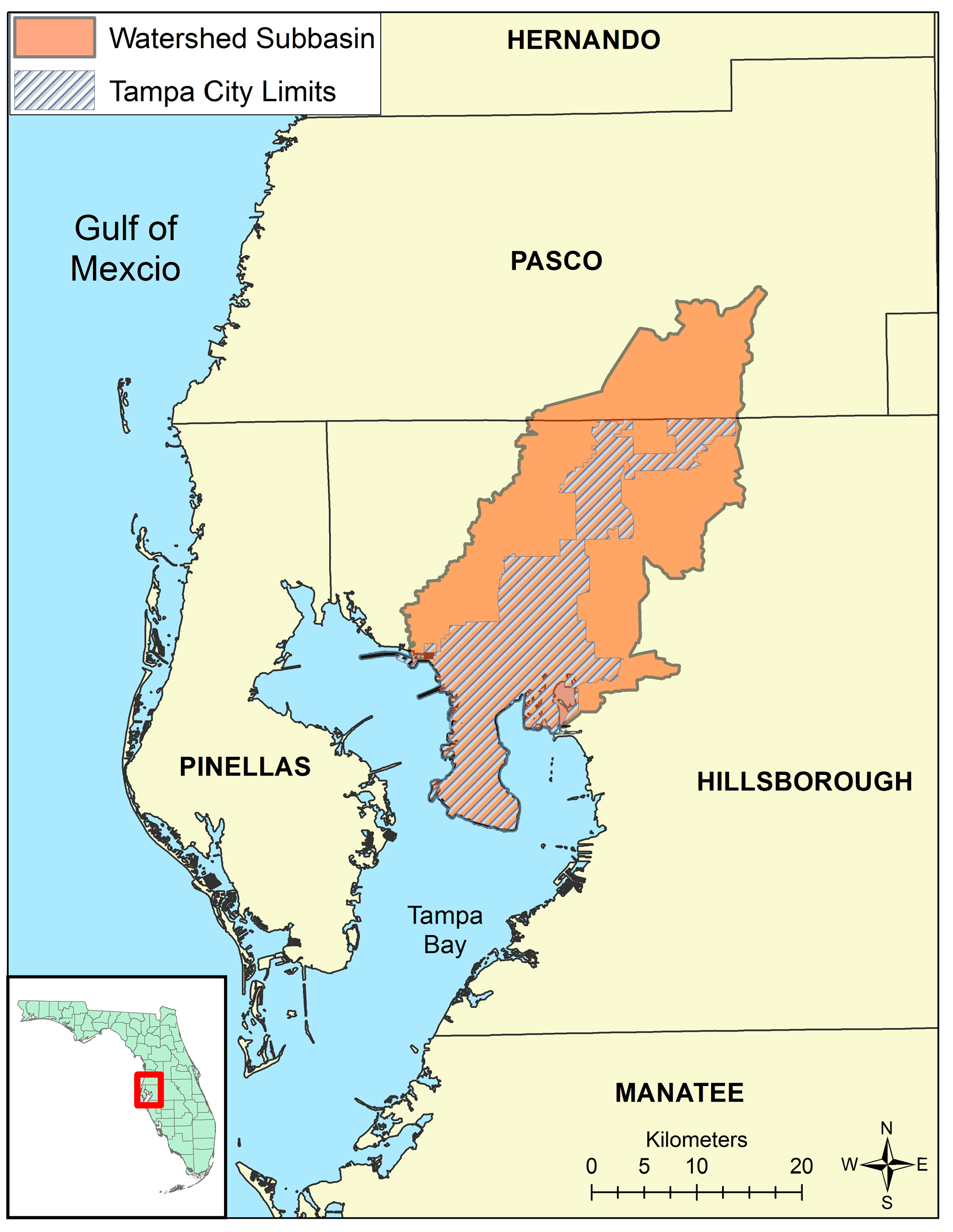
The analysis occurred in a 796-km2 subbasin of the Tampa Bay Watershed (TBW) in the state of Florida in the southeastern United States. The subbasin contains the entirety of the City of Tampa (population 377,000) and a portion of its surrounding area (Figure 1). The greater watershed area contains 4.6 million people and has seen rapid development adding 1,000,000 people over a ten year period beginning in the mid-1990s [35]. Commercial activities include phosphate mining, power generation, tourism, recreation, and agriculture, which have contributed significantly to land-use and land cover change [36]. For more details about the study area please see Lagrosa IV et al. [37].
2.2. Overview
Dyna-CLUE was used to project LULC change over a five-year period from 2012–2016. The five-year duration was selected because of the heterogeneous nature of urban landscapes in general, and the significant rates of urbanization in the TBW over the last 20 years [35]. The specific years 2012–2016 were selected because of data availability, with 2011 being the last published LULC dataset available from the Southwest Florida Water Management District (SWFWMD).
Land-use maps created by SWFWMD are shapefiles of polygons using a proprietary modification of the Florida Landcover Classification System [38,39]. These polygons are analogous to the “patches” described earlier. However, the CLUE framework, as with many simulation-based models operate in a per-pixel fashion. Therefore, LULC data were converted to raster format using a cell resolution of 100 m (spatial resolution of 1 ha).
2.3. CLUE Framework
The Conversion of Land-use and its Effects (CLUE) is an LULC change framework that has been used in national, regional, and small-scale studies to project landscape change. It has been applied by the European Environmental Agency to project LULC change on the European continent [40,41] and at national extents in Central America [42] and Ecuador [43]. It has been used to examine the effects of LULC change on alternative conservation policies in Chile [44], groundwater in Belgium [45], biodiversity in Northern Thailand [46] and urban renewal in Hong Kong [47] among others. The framework uses a hierarchical approach based on systems theory that combines total area analyses with those for individual spatial units. The framework creates projections of both the total quantity and distribution of land in each LULC class by coupling aggregate land-use requirements (demands) with a spatially explicit allocation procedure. The first iteration, CLUE-CR (1996), was developed to analyze multi-scale LULC change for Costa Rica [48], by integrating analyses at the national and regional scales. CLUE-S (2002) was later adapted from the original framework to model LULC change for watershed and other smaller regional extents, at finer spatial resolutions than the previous version [49]. CLUE-CR was developed to process landscape features represented at a resolution greater than 1 km, typical for national scale maps. However, smaller units of interest for highly heterogeneous landscapes, such as urban environments, have much finer resolutions typically smaller than 1 km [49]. The latest version Dyna-CLUE (2009), was designed to integrate top-down allocation with bottom-up dynamics of local drivers [50]. The “top-down” approach common in many modeling frameworks, uses an estimate of aggregate land requirements to simulate external, large-scale determinants of LULC change, while “bottom-up” refers to specific transition characteristics and driving factors of the local area [50].
2.4. Data Requirements
The CLUE framework is data intensive and requires significant preparation before analyses can proceed. However, the process of collecting and preparing data itself provides useful results and a better understanding of landscape dynamics in the study area. The first set of requirements are maps of restricted areas, or those areas that will not change during the temporal scale of the study. These are lands with spatial policies that prevent development. Common examples include county, state, and federal parks and zone restricted areas because of a particular land-use.
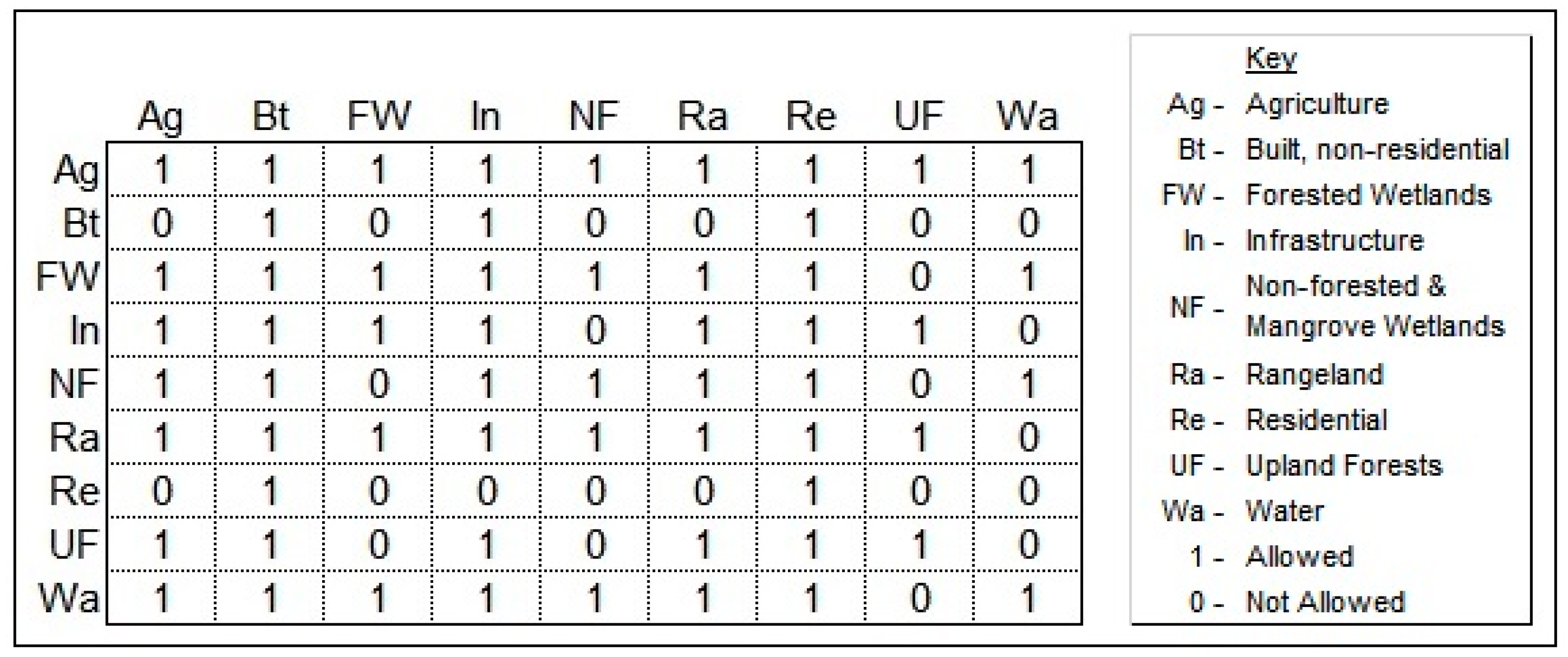
Land-use type conversion settings are needed for transition sequences and elasticities of classes. Transition sequences define the specific transitions each class can make. In a given study it might be possible for a “Forest” class to change into a housing development. However, it might not be possible for a “Residential” class, once developed, to transition into a wetland. Elasticity is an economic term that refers to an entity’s ability (or inability) to respond to external phenomena. Within an LULC change context it is the likelihood that a spatial unit of a specific class will change. Areas of high capital investment are one example [50]. Since these areas contain significant investment, their likelihood to change is low, even if other potential uses are theoretically possible. Stated another way, this means they have a high resistance to change. Each class receives a value between 0 (always convert) and 1 (never convert) and is used in conjunction with other input data for a given pixel of a given class to determine if change will occur. Ultimately, the elasticity and transition sequences function together, along with other input data, to control if a change will happen (elasticity), and if so, which change scenarios are possible (transition sequence).
The next inputs are aggregate land-use requirements (i.e., demand) for each class. These can come from many sources but are typically the result of an external economic model or trend extrapolation, if historical land-use data is available. The land requirements determine the total quantity of land area each class must occupy for each year of a simulation run. They are also an important feature of the framework because they can be manipulated to simulate management or economic scenarios that dictate an aggregate increase or decrease in land area for each class.
The last input data are landscape location characteristics. These characteristics, also known as driving factors, provide information specific to each land-use class. For each class, data on the driving factors of change must be collected and typically include such variables as population densities, soil characteristics, weather patterns, unique economic attributes etc. subject to the needs of each study area. This makes the model particularly suited to urban areas because the user can include and test potential anthropogenic variables of LULC change, so long as data defining these variables exist, are obtainable, and are spatially explicit for the entire study area. Often the collection, testing and conversion of these data require the most significant amount of time in parameterizing the model.
Once collected and formatted, the driving factors are used to develop a probability equation for each LULC class. This equation is used during the allocation procedure to derive a probability of change for each spatial unit. The theoretical equation for each pixel R, based on its location i, and driving factors X1 to Xn, is:
where “R is the preference to devote location i to land-use type k; X1→n,… are biophysical or socio-economical characteristics (driving factors) of location i; while ak and bk are the relative impact of these characteristics on the preference for land-use type k” [34], (6). Many statistical methods can be used to fit the probability equations. This study, as with many applications of the CLUE framework, uses a binomial logit regression to determine spatial probabilities [50].
Rki = akX1i + bkX2i + …
2.5. Simulation Process
The total probability of change for each cell is based on the LULC classes of surrounding cells (land-use allocation) and the decision rules set by the user. The theoretical equation for a given pixel in the model is defined as:
where TPROPi,u is the total probability of change for any cell i for one of the 9 land-use classes u. Pi,u is the initial probability for each cell calculated from a set of driving factors derived from the input data [41]. ELASu is the elasticity, or sensitivity to change based on the decision rules for each class. ITERu is an iterative variable distinct for each land-use class. The model runs in annual increments. Each annual step is one iteration of the simulation. When the model is initialized, all classes start with an equal value of ITERu. After every iteration, the new allocation for each class is compared to its land-use requirement specified in the non-spatial module. If the allocation of a land-use class u is smaller than its requirement, the value of ITERu increases, causing the model to repeat the allocation calculation process until the requirement equals allocation, subject to the class’s elasticity and driving factors. Conversely, ITERu decreases if the allocation exceeds the class’s requirement until demand and allocation are equalized.
TPROPi,u = Pi,u + ELASu + ITERu
2.6. Restricted Areas
The model specifies the designation of restricted lands, or those with little to no likelihood of change within the timeframe of the study. These are commonly thought of as conservation areas and land with legal restrictions that prevent change. Examples include local, county and state parks; ecological reserves; private lands held as trusts and protected trail networks.
An important consideration with restricted lands is the context of the study. These are not lands in which change is impossible, but merely restricted and unlikely to change during the time-period under investigation. Even restricted lands can contain parcels that change as areas are developed for various purposes (i.e., visitor centers, research facilities etc.) or altered for ecological restoration. In addition, other public or private lands that are designated for very specific purposes can be considered “restricted” if their purpose prohibits alteration. One example is cemeteries. Although cemeteries can experience meaningful change overtime (conversion of grass space to concrete cover) the magnitude of change is dependent upon the timeframe of the study [51].
Seven spatial datasets were used to determine areas restricted from LULC change during the timeframe of analyses. The datasets were processed in ArcGIS [52] to create a single master shapefile of restricted lands. This layer was used as an input parameter for the model in the spatial allocation procedure.
The following datasets were used to process this layer (Table 1): Florida State Parks [53], Local and County-owned Parks and Recreational Areas [54], Public and Private Managed Conservation Lands [55], Publicly Managed Pinelands [56], Current SWFWMD Managed Land [57], Florida Cemetery Facilities [58], and Existing Florida Trails [59].
2.7. Driving Factors
Urban areas are influenced by many variables, both ecological and anthropogenic [19], far more than most models will accept or for which data is available. Eight driving factors were included in the model, based on available data in three categories: demographic, economic, and environmental (Table 2). Driving factors in the CLUE framework can be either static or dynamic. Static variables refer to those that are consistent for each simulation year whereas dynamic can change from year to year. The only dynamic variables used for this study were population densities. Density estimates for each year were calculated from population data obtained from the 2010 United States Census [60] and 2013 American Community Survey [61]. Populations for years in between and after were estimated using an annual growth rate of 1.57%. This rate was estimated for Hillsborough County by the Florida Office of Economic and Demographic Research [62]. Seven other static driving factors were included as possible drivers of LULC change in the model (Table 2): enterprise zones [63], parcel structure values and parcel structure ages [64], flood hazard areas [65], USGS soil survey [66], EPA Superfund sites [67] and road presence [68]. Soil series type initially contained 60 levels corresponding to officially designated USGS soil series classifications found in the subbasin [66]. To briefly summarize, Basinger series comprised 22.33% of the area followed by Myakka (8.72%), Malabar (6.22%), Zolfo (4.56%), and St. Johns (4.21%). The remaining 55 types represented between 0.02% and 3.1%, respectively. To reduce model complexity, this frequency range was used to recategorize these levels into a single “Other” category, for a final count of 6 levels.
A binomial logit model was used to test each of the 8 driving factors (α = 0.05) and calculate the spatial probability of change for each pixel in the subbasin. A regression was fit for each LULC class using the following theoretical equation:
where P is the probability that a pixel will change to class i based on each static driving factor Xn and its modeled coefficients, β1→n. The logistic transformation of the probability ratio results in an odds value that represents the likelihood of success or failure, in this case pixel conversion [69]. Receiver-operating characteristic (ROC) curves were calculated using the predicted probabilities to evaluate the goodness of fit for each class equation. The area under an ROC curve ranges from 0.5 (completely random) to 1 (perfect fit) and is an indication of overall model performance.
2.8. Conversion Settings
The model requires a transition matrix that specifies possible class conversions. Allowable sequences are set based on the possibility of conversion between two classes within the temporal context of the study. These were derived by interpretation of conversions using SWFWMD maps on a year-to-year basis.
In addition to allowable transitions, an elasticity of change for each class is required to determine the likelihood and/or difficulties in pixel conversions for each class. Elasticity values (Table 3) were determined from the literature by aggregating and adapting established values from previous applications of the CLUE framework [70,71,72,73].
2.9. Land-Use Requirements
Dyna-CLUE primarily functions as an allocation model, determining spatial location and distribution of LULC change given land-use requirements. These land-use requirements or demands are specified as inputs to the allocation procedure. They represent the total estimated area for each LULC class after successive iterations of the model. Trend extrapolation using the Geomod approach [24] was used to estimate the land-use requirements based on 10 years of historical land-use data over a 16-year period from the SWFWMD LULC datasets. The original LULC classes were reclassified using an ecosystem services-centric classification scheme that uses ecological data to determine spatial variation [37]. They were then converted to raster format and expansion/reduction trends were extrapolated in ArcGIS incrementally for each year. Linear slopes to calculate changes in land area between successive years of historical data were used to estimate a matrix of area quantities for each LULC class used to determine quantity changes over the five simulation years (2012–2016).
3. Results
3.1. Restricted Areas
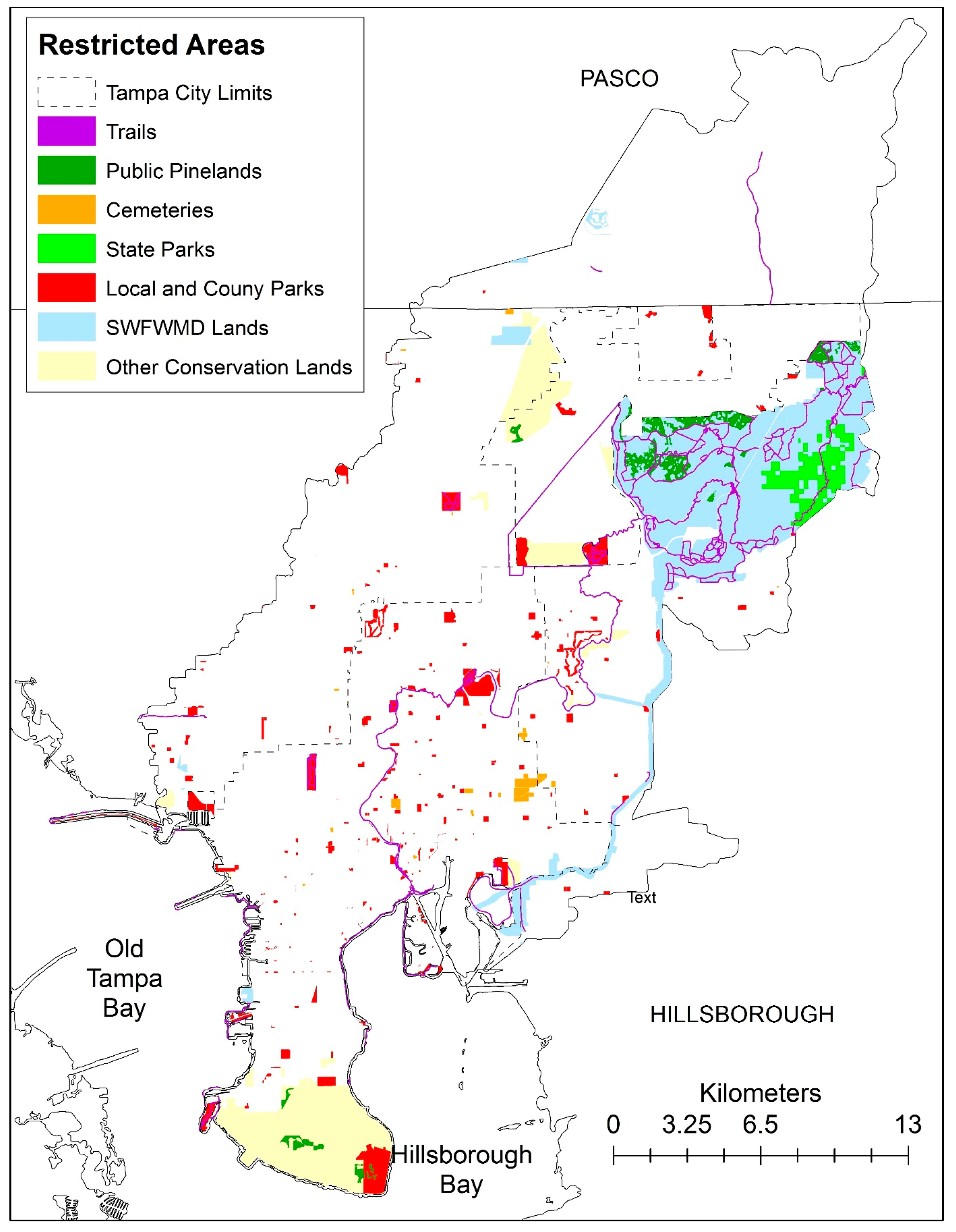
Restricted areas covered 13,492 ha of the subbasin or approximately 17% of the total land area (Figure 2). About 5939 ha occurred in or adjacent to the 654 ha Hillsborough River State Park in the north-eastern portion of the subbasin and contained large areas of upland forests and forested wetlands. An area of restricted land nearly 2500 ha occurred in and around MacDill Air Force Base at the southern tip of the City of Tampa. Most of this land occurred on non-forested wetlands or built sections of the base.
Overall, SWFWMD was responsible for the management of 53% of restricted land. Other public and privately managed conservation land was almost 20%. Local and county-owned parks comprised 12% while the other four categories collectively held the remaining 15% (Table 4).
3.2. Driving Factors
Each binomial logit model had its own set of driving factors (Figure A1). “Rangeland” had the smallest number with only flood risk, structure age, and soil type as predictors of LULC change. “Built, non-residential” and “Upland Forests” were next with four each, including enterprise zone, structure age, and soil in both equations. All eight potential variables were significant predictors for the “Residential” class, which was the only class with population density in the final model. The “Forested Wetlands”, “Infrastructure”, “Non-forested Wetlands”, and “Water” classes all had the remaining seven variables in their models. Soil type and structure age were significant predictors for every class model while enterprise zone (“Rangeland”) and flood risk (“Built, non-residential”) were in seven of eight. Roads were a useful predictor in all but the “Rangeland” and “Upland Forests” classes.
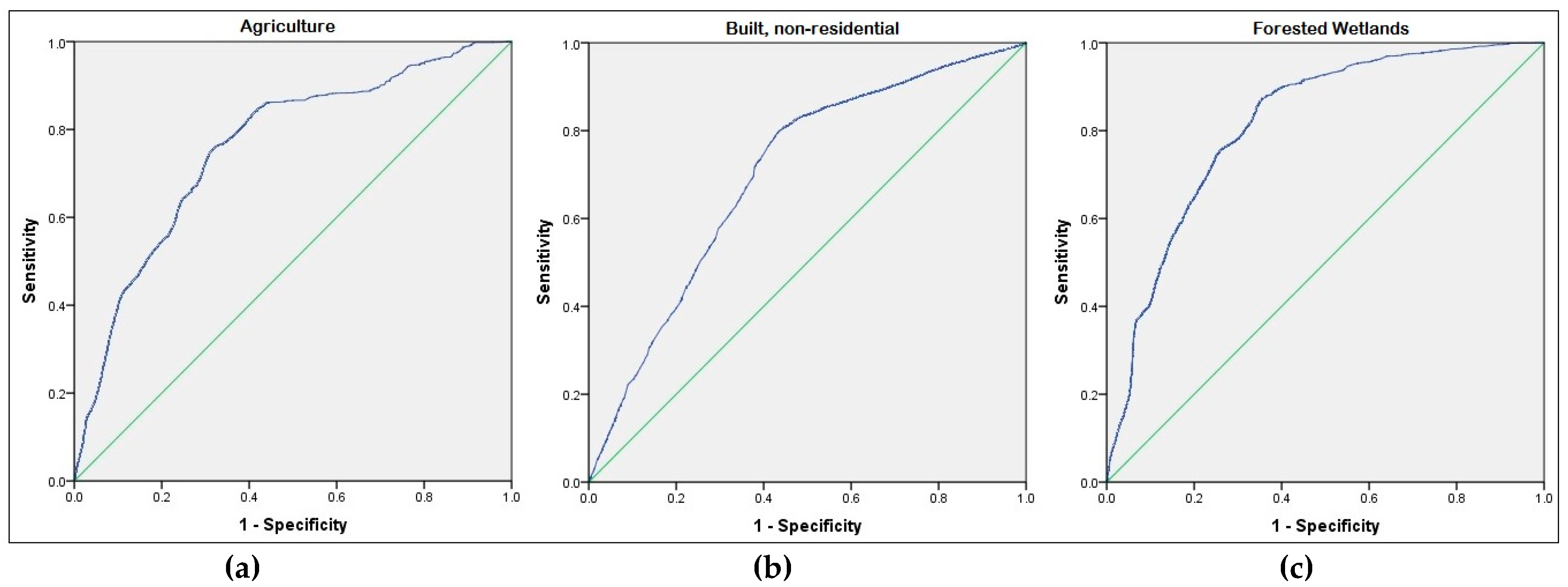
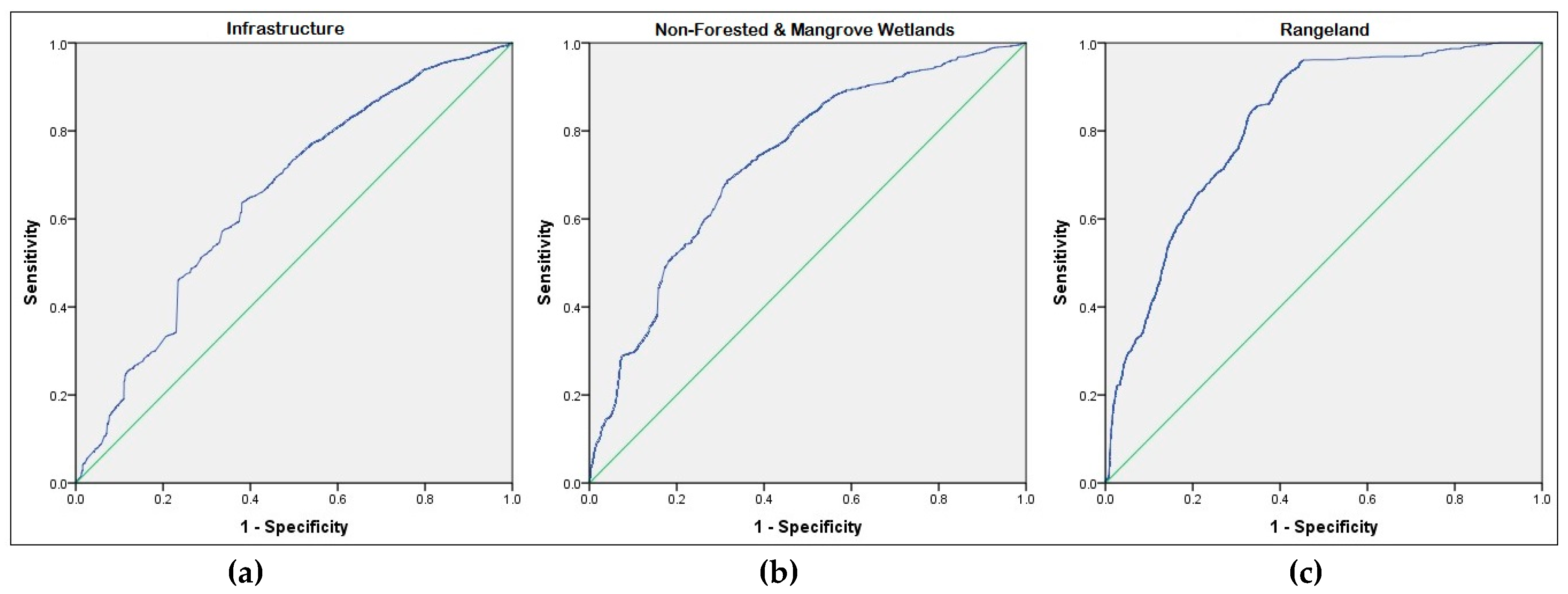
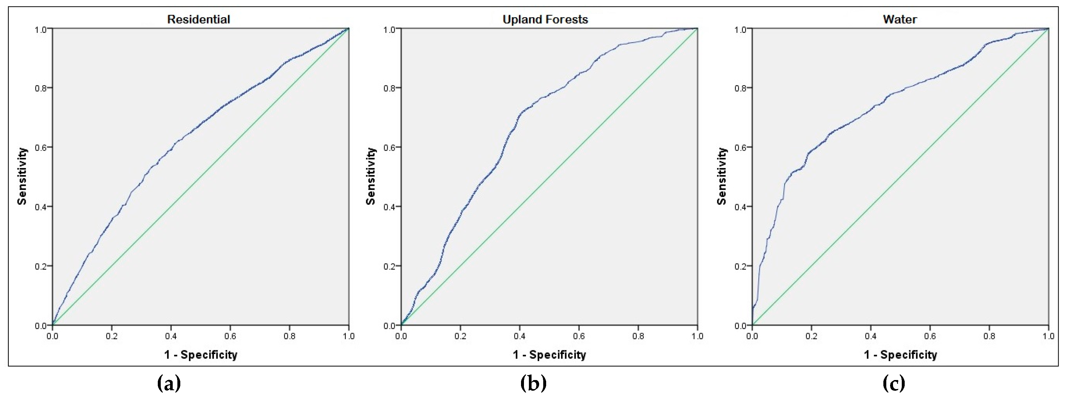
ROC results ranged from 0.63 (“Residential”) to 0.83 (“Rangeland”). “Forested Wetlands” had an ROC area of 0.82. Four other models ranged from 0.70 to 0.77 (“Agriculture”, “Built, non-residential”, “Non-forested and Mangrove Wetlands”, and “Water”). “Upland Forests” and “Infrastructure” had values of 0.68 and 0.66 respectively (Table 5, Figure A2, Figure A3 and Figure A4).
3.3. LULC Change
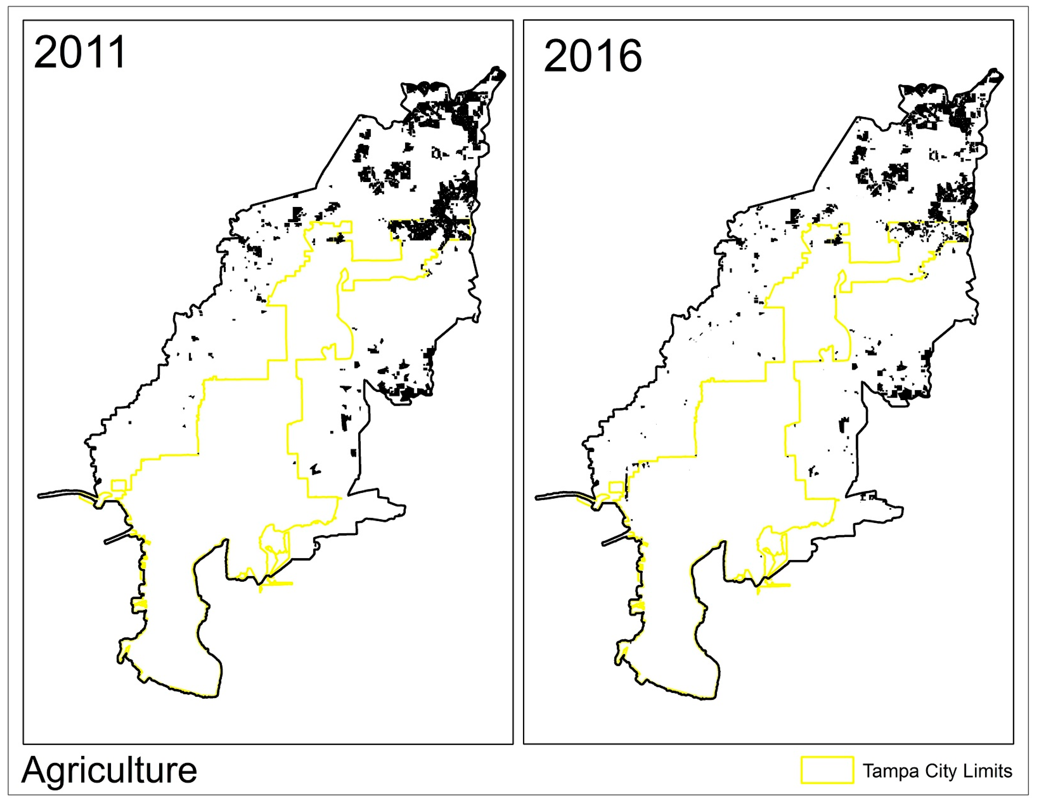
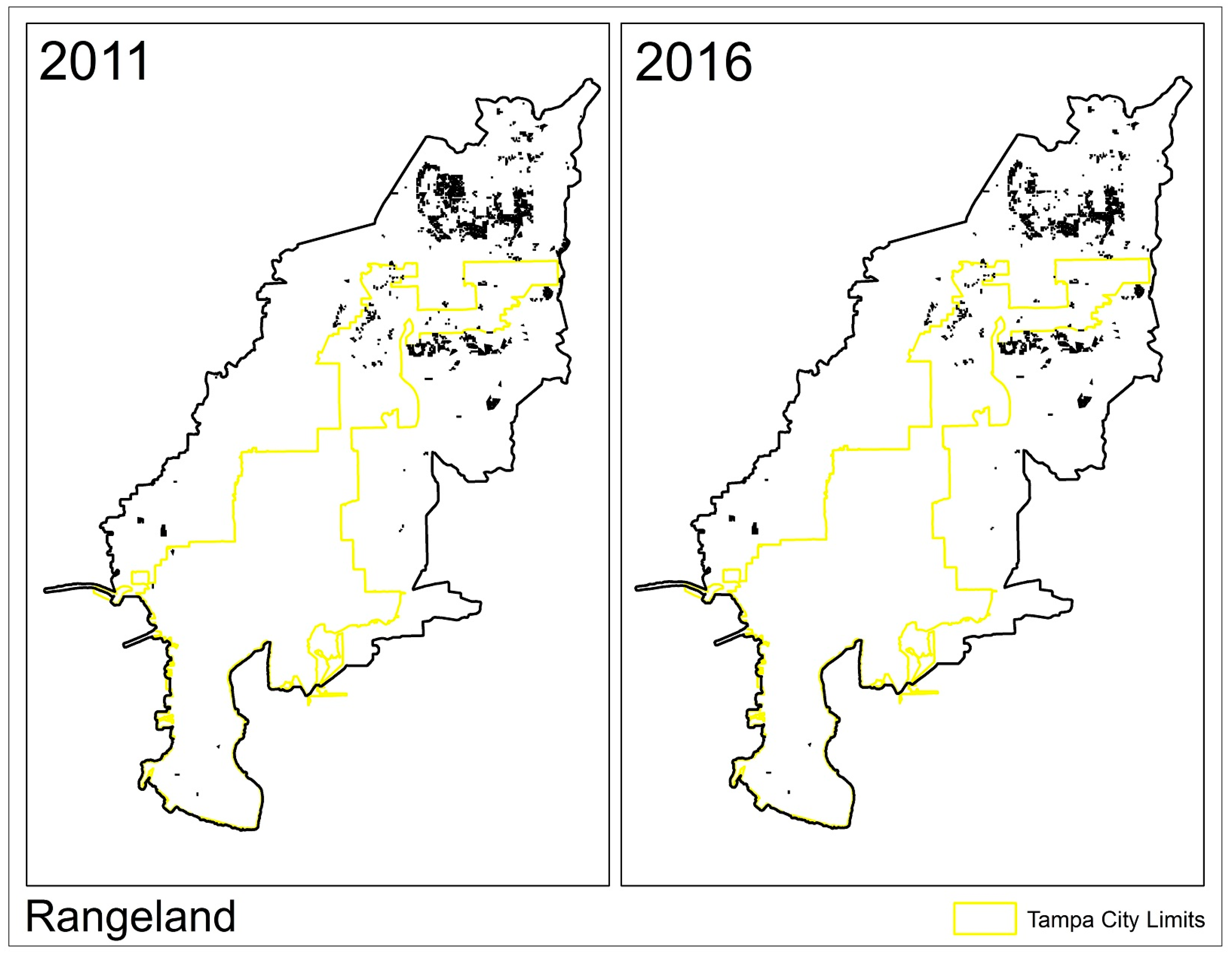
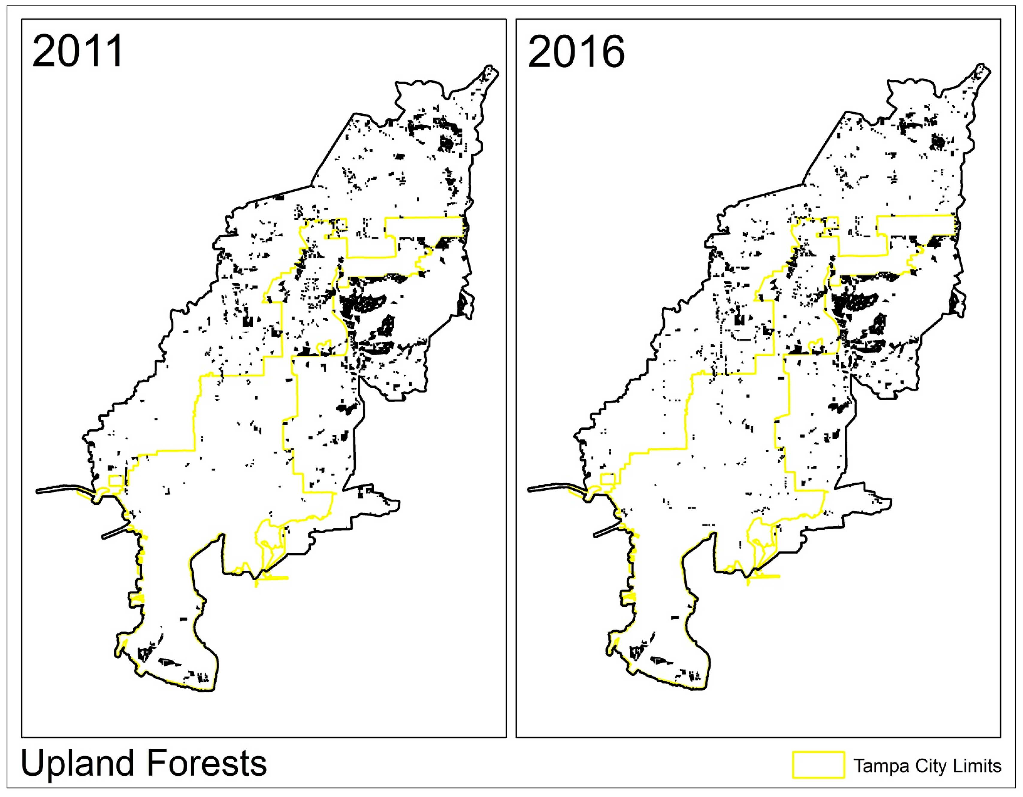
The observed changes in area from the SWFWMD data show a 49% decrease in “Agriculture” between 1995 and 2011 from 89 km2 to 45 km2 (Table 6). However, 82% of this decrease occurred between 1995 and 2006. This trend slowed significantly in 2007 with only a 3 km2 difference between 2007 and 2011. Similarly, “Rangeland” had a 56% decrease in land area from 46 km2 in 1995 to 20 km2 in 2011 with 81% of this occurring between 1995 and 2004. From 2004–2011 there was only a 5 km2 decrease in “Rangeland” with no loss in total area for the most recent three years of data (2009–2011). “Upland Forests” experienced a 27% (16 km2) decrease from 1995–2011, again with the majority (75%) occurring between 1995 and 2004.
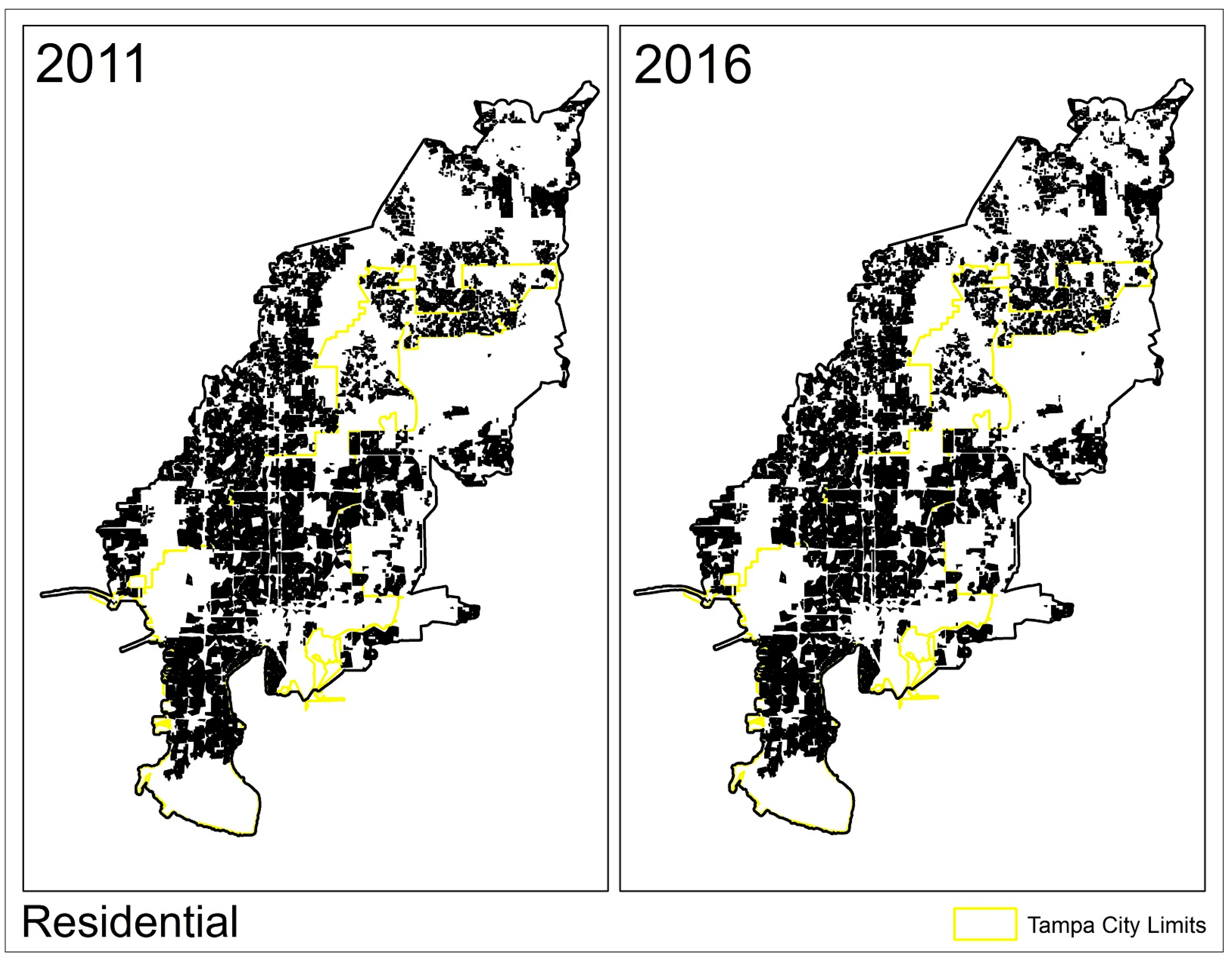
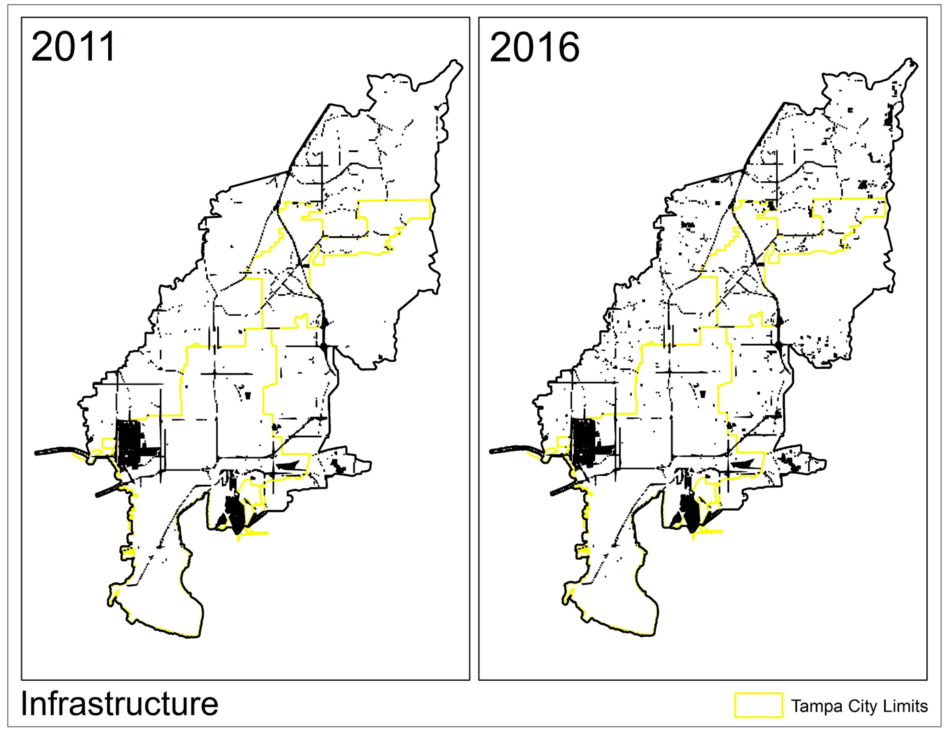
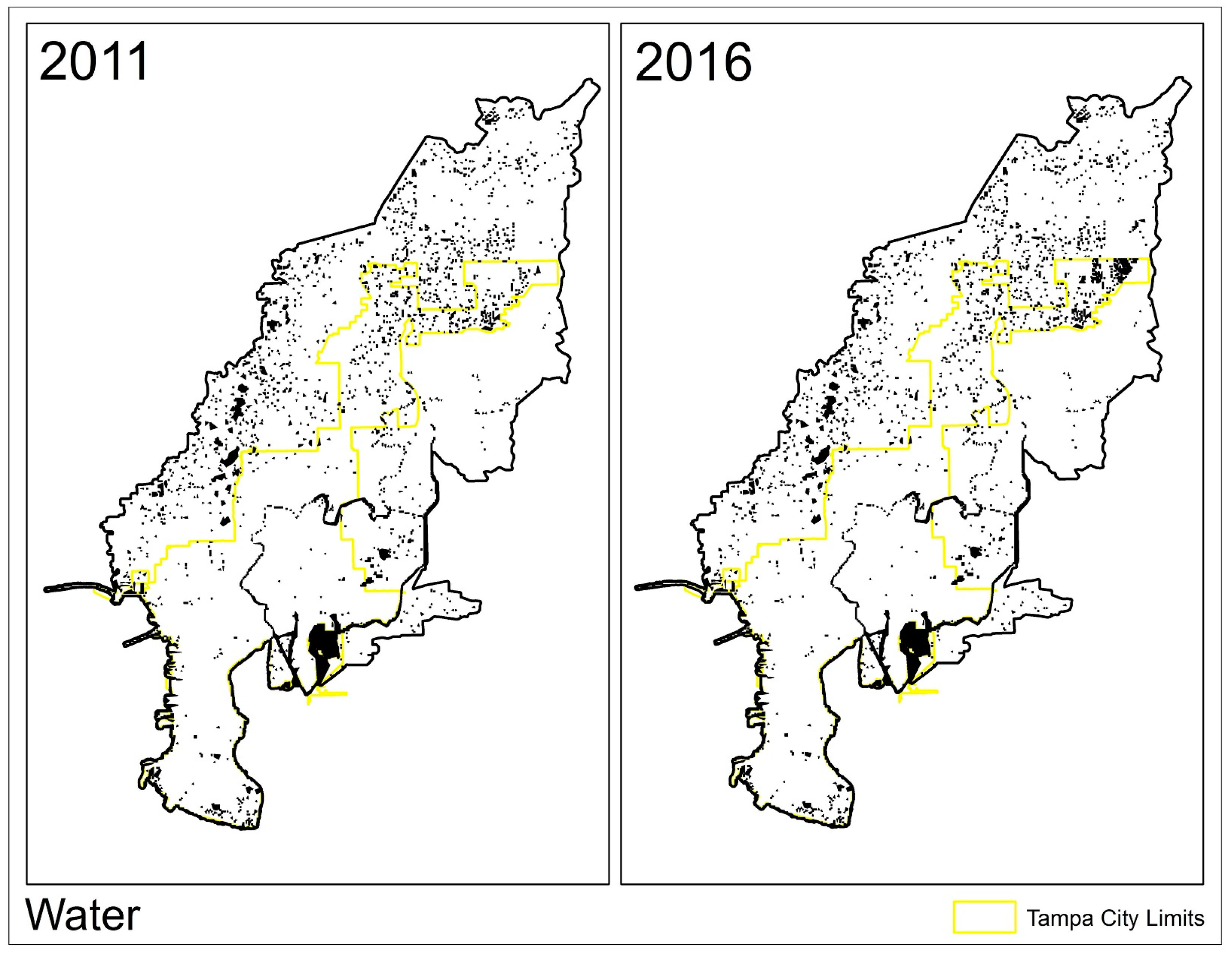
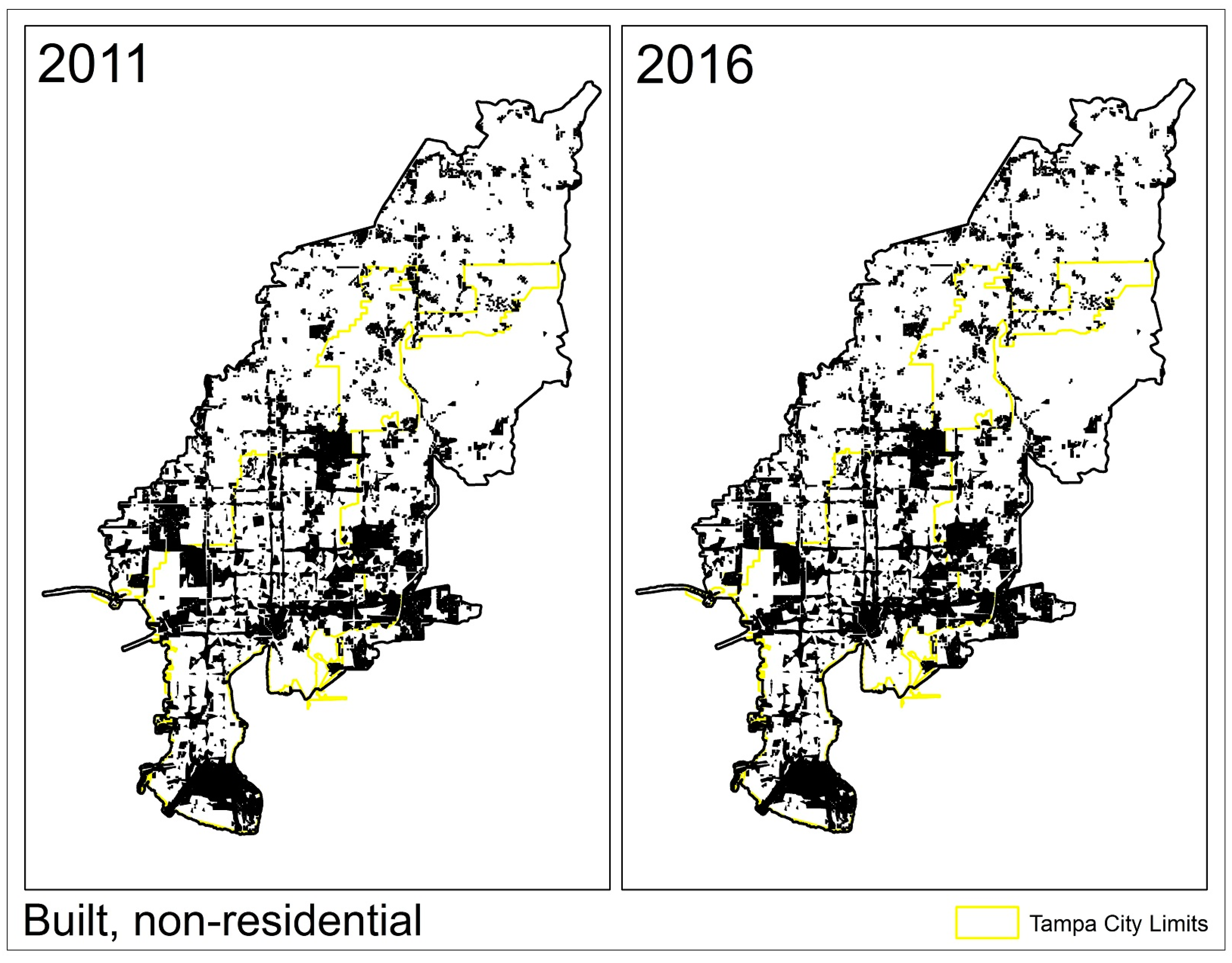
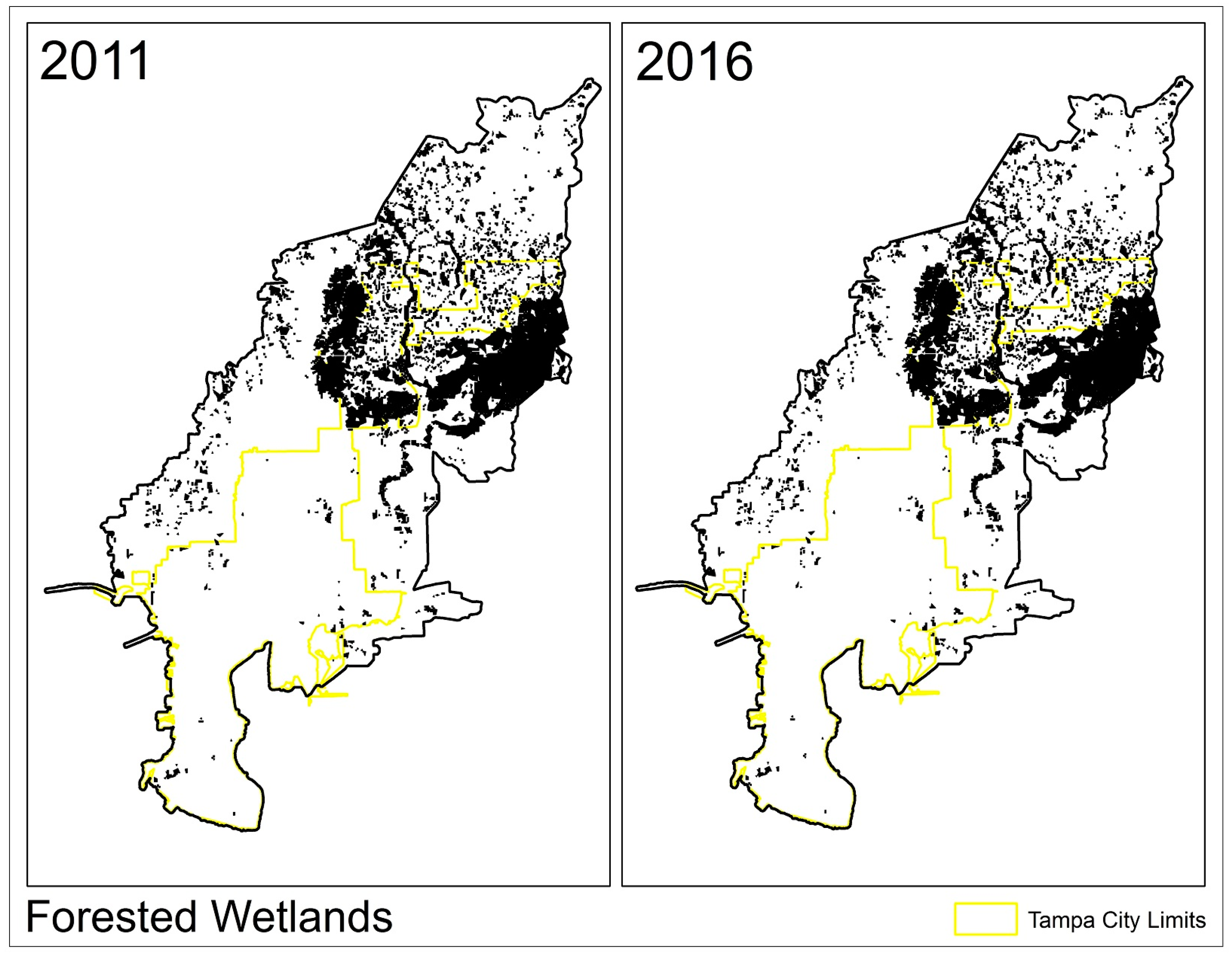
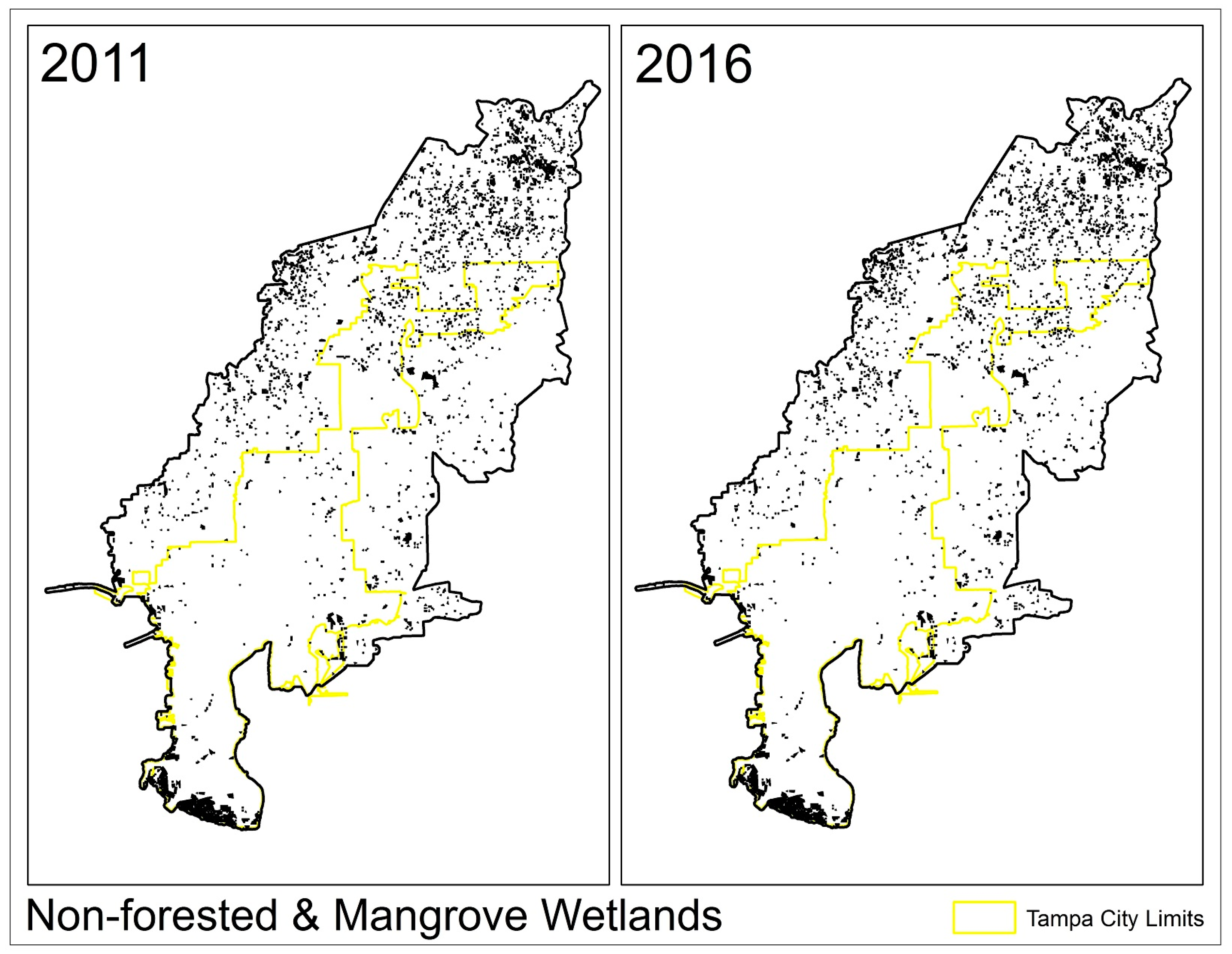
The six remaining classes showed a net growth over the sixteen-year period of observable data (Table 6). “Residential” had the greatest absolute increase from 214 km2 to 262 km2 or 22%. “Water” had the highest relative increase of 25% growing from 40 km2 in 1995 to 50 km2 in 2011, followed by “Infrastructure” (23%), which grew from 39 km2 to 48 km2. “Built, non-residential” was next with an 8% increase followed by “Forested Wetlands” (6%), and “Non-Forested Wetlands” (2%). The intensity of this growth followed a similar pattern to the loss in area of the first three classes with the greatest proportion of change occurring from 1995–2004.
Projected land-use requirements for 2012–2016 (Table 7) were based on trends of the preceding five-years (2007–2011). The “Agriculture”, “Rangeland” and “Upland Forests” classes were projected to decrease by 9%, 15% and 8% respectively. “Residential”, “Infrastructure” and “Non-forested Wetlands” each had an increase of 11%, 8% and 5%, respectively. Finally, “Built, non-residential”, “Forested Wetlands”, and “Water” remained relatively steady over the five-year period.
The spatial allocation determines changes in the distribution of patches for each LULC class (Table 8, Figure A6, Figure A7, Figure A8, Figure A9, Figure A10, Figure A11, Figure A12, Figure A13 and Figure A14). The decreases in “Agriculture”, “Rangeland” and “Upland Forests” primarily occurred toward the north-northeast of the study area with some loss near or within City of Tampa boundaries (Figure A6, Figure A7 and Figure A8). Land area increases for the “Residential” classes were mostly restricted to the northeast as well (Figure A9). The increase in “Infrastructure” area occurred throughout the subbasin on relatively small patches and mainly near the edges (Figure A10) while the increase in “Water” occurred in the eastern-most portion of the City of Tampa (Figure A11). The “Built, non-residential”, “Forested Wetlands”, and “Non-forested and Mangrove Wetlands” classes had very little change in total land-use demand and similarly very little change in distribution and allocation of class patches (Figure A12, Figure A13 and Figure A14).
Modeled LULC change also projected a change in the distribution and mean size of landscape patches (Table 8). The “Agriculture” class went from 227 patches in 2011 with an average patch size of 20.05 ha to 401 patches at an average of 9.38 ha in 2016. “Infrastructure” increased from 796 patches to 1098, with a slight decrease in size from 5.96 ha to 4.66 ha. The “Residential” class increased from 565 patches to 641 with a decrease in mean patch size of 4.56 ha. The other LULC classes had minimal changes in both patch count and mean patch size from 2011–2016 (Table 8).
4. Discussion
In total, the land area of the subbasin corresponded to 796 km2 or 79,600 pixels (1 pixel = 1 ha). For model parameterization, two other resolutions were explored: 30 m and 250 m. The 30 m resolution was too fine and unable to cover the spatial extent of some driving factors, namely population density, and increased the pixel count to near 240,000. The coarse scale of 250 m was found to aggregate many patches that were smaller than 250 m but of different LULC types. The 100 m resolution was selected in an attempt to alleviate information loss associated with finer or broader spatial resolutions.
Beta coefficients in binomial logit models are not as easily interpreted as those in other forms of regression [69]. However, a few interpretations can be made by looking at their relative value and sign. The binomial logit model yields a logistic transformation of a probability ratio. The ratio itself gives the probability of change for a given pixel while the logistic transformation gives an odds value. Therefore, we know that the betas are influencing a pixel’s likelihood of change with the coefficient’s sign influencing the direction of probability. For example, structure age was significant as a predictor of change for built areas. However, the effect was negative, suggesting that built areas are less likely to change as their structures age. One would assume the opposite; that as buildings age, there is a higher likelihood they will be torn down and replaced or renovated, cet. par.
Structure value was not a statistically significant factor for many classes. This may be because the magnitude of value, once a building is established, has very little to do with influencing LULC change between classes. That is to say, a building of any value is more likely to be purchased and rebuilt into another structure than converted to a new class. Road presence in built areas was shown to cause a decrease in the probability of a pixel’s change. Perhaps this is because roads almost always coincide with built structures for access, and once established, stabilize the land-use of parcels around them. This was similar for the “Infrastructure” class. However, the “Residential” class showed a positive relationship with road presence. “Agriculture” and the two wetland groups also had a positive relationship with roads, which indicates that the presence of roads is tied to future LULC change in those areas. Roads were not significant in the “Rangeland” and “Upland Forests” classes but were significant in the two wetland classes. Enterprise zones had a positive relationship with all classes except “Residential” and “Infrastructure” (negative for both) and “Rangeland” (not significant). This indicates that the establishment of an enterprise zone may positively increase the probability of change for non-built areas. Soil type is a commonly used predictor in many LULC change studies and these results support that conclusion. Population density was only significant for “Residential”, which was the only class that had a significant permanent population.
ROC areas ranged from 0.63 to 0.83 (Table 5). Ideally these values should be as close to 1 as possible. Values less than 0.6 are typically viewed as inadequate models and values of 0.6 to 0.69 as poor. Values of 0.7 and higher are usually seen as useful models. Six of the nine models had values of 0.7 or higher, while three had values in the 0.63 to 0.68 range, which indicates that better, or possibly more predictors are needed for those classes [69].
Model results were consistent with previous work that shows most LULC change in urban areas occurs on the fringes of the urban environment with the replacement of rural and agricultural land by residential development [74]. Development of low-density exurban land occupies an area 15 times higher than development in high-density urbanized landscapes, particularly east of the Mississippi River where exurban land has declined 22% between 1950 and 2000 [75]. Theobald [76] describes this as “exurban sprawl” (contrasted with urban sprawl), and forecasted that urban and suburban housing densities would expand 2.2% compared to 14.3% in exurban landscapes throughout the U.S. by 2020. Theobald [77] also found that the majority of LULC studies focus on development within urbanized areas, often ignoring exurban areas, despite their observed importance in overall LULC change.
For the TBW subbasin “Agriculture”, “Rangeland”, and “Upland Forests” showed significant decreases in land area, whereas both wetland classes were mostly unchanged. This study did not investigate the dynamics of change within individual LULC classes, but possible reasons include both economic and cultural [75,78,79]. Building in wetlands necessitates draining and clearing to create firm ground for construction. Dryer areas, including those with upland vegetation, only require clearing. Restoration ecology of upland forests, particularly longleaf pine, has also received considerable attention by conservation groups and local organizations [80]. Theobald [81] modeled landscape dynamics for the conterminous U.S. using a proportion cover approach and estimated that in 1992 2.6 million km2, or 1/3 of the U.S. was human-dominated. He projected that by 2030 an additional 173,000 km2 of natural areas will be lost due to residential expansion, with 21.7% of wetland areas and 15.1% of forested lands affected, which ranked first and second respectively of the five natural LULC classes used in the study [81].
The decrease in “Agriculture” reflects local trends shown in available data since 1995. Decreases in “Agriculture” and “Rangeland” coincided with an increase in the “Residential” class. In all cases, the positive and negative trends slowed significantly around 2007. It is possible this reflects the slow-down in housing markets associated with the national recession, which peaked in 2008. Prior to the recession, the national economy was experiencing inflated rates of home construction and real estate sales, followed by a market crash and economic stagnation. An investigation into a connection between decreased rates of LULC change and the economy during the study timeframe would be useful. Understanding the influence of the market economy on regional LULC dynamics would have important implications for future models. However, this slow-down in residential development is not projected for the future of the region. Russell et al. [82] summarize research and projections into the future of development in west-central Florida and conclude that “explosive” development of the Interstate 4 and Interstate 75 corridor (considered the region that includes Tampa and Orlando and named for the junction of the two highways between both cities) will lead to a rapid decline in agriculture and natural landscapes over the next 20 years.
Most classes were consistent in their direction of change from year-to-year (i.e., increase or decrease). The “Built, non-residential” class showed a 7 km2 increase from 1999–2004 and 3 km2 decrease from 2004–2005. From 2005–2009 it increased by 6 km2 with a 2 km2 decrease in both 2010 and 2011. Two other classes showed a fluctuation in their direction of change (“Forested Wetlands” and “Water”) but only for one year and of 1 km2.
A few basic parameters of patch dynamics were provided. The number of discrete patches and patch areas shows that fragment distribution in the TBW subbasin is increasing overtime. A number of additional metrics and tools exist to investigate current and future landscape patch distributions, but these analyses were outside the scope of this study. However, further fragmentation analyses would serve as a useful follow-up to better understand the nature of LULC change and its internal dynamics.
In summary, sixteen socio-ecological datasets from eleven local, state and federal agencies were used to parameterize the Dyna-CLUE LULC modeling framework. Landscape-scale class area requirements were derived from 10 years of LULC data provided by the Southwest Florida Water Management District. Binomial logit regression was used to test a set of eight possible drivers of LULC change. Finally, elasticities and transition sequences were adapted from the literature to characterize the direction of change (Figure A6). Observed data from 1995–2011 showed a decrease in land area for “Agriculture”, “Rangeland” and “Upland Forests” by 49%, 56% and 27% respectively. This coincided with a 22% increase in residential and 8% increase in built areas, primarily between 1995 and 2004. Modeled LULC change showed a continued reduction in “Agriculture” and “Rangeland”, alongside an expansion of “Residential” and “Infrastructure”. In addition to total quantity, most classes experienced some changes in patch size and distribution. The “Agriculture” class had a 77% increase in the number of patches with a 53% decrease in patch size. “Infrastructure” had a 38% increase in the number of patches with a 22% decrease in mean patch size while “Residential” had a 13.5% increase and 10% decrease respectively. Urban areas in the subbasin occurred along a gradient moving southwest to northeast, with the most concentrated areas of development in the south near Tampa Bay. The most significant areas of change occurred in the northeastern portion of the subbasin adjacent to suburban, exurban, rural and natural areas.
As mentioned, the drivers of LULC change in urban areas can potentially number into the hundreds or more, if they can even be identified at all. This study was limited in both data and information on the dynamics and drivers of LULC change in the TBW. Further analyses in variable selection would contribute greatly to the accuracy of the LULC change model. To account for the rapid rate of change in urbanizing areas, as well as the temporal availability of data, the LULC change model was restricted to a five-year projection. Although urban areas are heterogeneous and rapidly changing environments, it is unknown how the limited temporal scale impacts resulting conclusions.
Finally, a comprehensive validation of the model was beyond the scope of this paper. While the CLUE framework has been validated by its authors and used in many regional scale studies, as cited throughout the paper, we seek to address model evaluation beyond ROC curves in future iterations. This was particularly challenging due to available LULC data, given the short time-span (5-years) of the study. As SWFWMD releases additional years of observed data, we hope to increase the quantity and scale of analyses that will provide a vehicle to compare future and past results, including validation, increasing accuracy over time.
Acknowledgments
We are thankful for funding support from the USDA Forest Service, City of Tampa, and School of Forest Resources and Conservation at the University of Florida. We would also like to thank Timothy A. Martin, Wendell P. Cropper, and Michael W. Binford for feedback on early drafts of the manuscript.
Author Contributions
J.L., W.Z., and M.A. conceived the study and collected data. J.L. performed the analyses and wrote the paper.
Conflicts of Interest
The authors declare no conflict of interest.
Appendix A
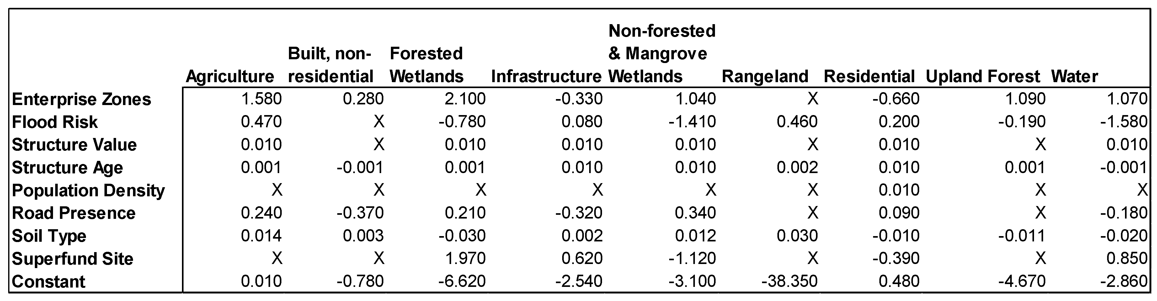
Figure A1.
Statistically significant beta coefficients of driving factors for each LULC class. If a coefficient is absent (X) it was not statistically significant at α = 0.05.
Figure A1.
Statistically significant beta coefficients of driving factors for each LULC class. If a coefficient is absent (X) it was not statistically significant at α = 0.05.

Figure A2.
Receiver-operating characteristic (ROC) curves to evaluate binomial logistic regression models of driving factors for (a) “Agriculture”, (b) “Built, non-residential”, and (c) “Forested Wetlands” classes.
Figure A2.
Receiver-operating characteristic (ROC) curves to evaluate binomial logistic regression models of driving factors for (a) “Agriculture”, (b) “Built, non-residential”, and (c) “Forested Wetlands” classes.

Figure A3.
Receiver-operating characteristic (ROC) curves to evaluate binomial logistic regression models of driving factors for (a) “Infrastructure”, (b) “Non-forested & Mangrove Wetlands”, and (c) “Rangeland” classes.
Figure A3.
Receiver-operating characteristic (ROC) curves to evaluate binomial logistic regression models of driving factors for (a) “Infrastructure”, (b) “Non-forested & Mangrove Wetlands”, and (c) “Rangeland” classes.

Figure A4.
Receiver-operating characteristic (ROC) curves to evaluate binomial logistic regression models of driving factors for (a) “Residential”, (b) “Upland Forests”, and (c) “Water” classes.
Figure A4.
Receiver-operating characteristic (ROC) curves to evaluate binomial logistic regression models of driving factors for (a) “Residential”, (b) “Upland Forests”, and (c) “Water” classes.

Figure A5.
Transition sequences matrix showing possible LULC class conversions.

Figure A6.
Observed (2011) and Modeled (2016) LULC distribution for the “Agriculture” class.

Figure A7.
Observed (2011) and Modeled (2016) LULC distribution for the “Rangeland” class.

Figure A8.
Observed (2011) and Modeled (2016) LULC distribution for the “Upland Forests” class.

Figure A9.
Observed (2011) and Modeled (2016) LULC distribution for the “Residential” class.

Figure A10.
Observed (2011) and Modeled (2016) LULC distribution for the “Infrastructure” class.

Figure A11.
Observed (2011) and Modeled (2016) LULC distribution for the “Water” class.

Figure A12.
Observed (2011) and Modeled (2016) LULC distribution for the “Built, non-residential” class.
Figure A12.
Observed (2011) and Modeled (2016) LULC distribution for the “Built, non-residential” class.

Figure A13.
Observed (2011) and Modeled (2016) LULC distribution for the “Forested Wetlands” class.

Figure A14.
Observed (2011) and Modeled (2016) LULC distribution for the “Non-forested & Mangrove Wetlands” class.
Figure A14.
Observed (2011) and Modeled (2016) LULC distribution for the “Non-forested & Mangrove Wetlands” class.

References
- Verburg, P.H.; Neumann, K.; Nol, L. Challenges in using land use and land cover data for global change studies. Glob. Chang. Biol. 2011, 17, 974–989. [Google Scholar] [CrossRef] [Green Version]
- Vitousek, P.M. Global environmental change: An introduction. Annu. Rev. Ecol. Syst. 1992, 23, 1–14. [Google Scholar] [CrossRef]
- Kalnay, E.; Cai, M. Impact of urbanization and land-use change on climate. Nature 2003, 423, 528–531. [Google Scholar] [CrossRef] [PubMed]
- Lambin, E.F.; Turner, B.L.; Geist, H.J.; Agbola, S.B.; Angelsen, A.; Bruce, J.W.; Coomes, O.T.; Dirzo, R.; Fischer, G.; Folke, C. The causes of land-use and land-cover change: Moving beyond the myths. Glob. Environ. Chang. 2001, 11, 261–269. [Google Scholar] [CrossRef]
- Turner, B.L.; Lambin, E.F.; Reenberg, A. The emergence of land change science for global environmental change and sustainability. Proc. Natl. Acad. Sci. USA 2007, 104, 20666–20671. [Google Scholar] [CrossRef] [PubMed]
- Foley, J.A.; DeFries, R.; Asner, G.P.; Barford, C.; Bonan, G.; Carpenter, S.R.; Chapin, F.S.; Coe, M.T.; Daily, G.C.; Gibbs, H.K. Global consequences of land use. Science 2005, 309, 570–574. [Google Scholar] [CrossRef] [PubMed]
- Hooke, R.L.; Martín-Duque, J.F.; Pedraza, J. Land transformation by humans: A review. GSA Today 2012, 22, 4–10. [Google Scholar] [CrossRef]
- Marsh, G.P. Man and Nature, 1965 ed.; University of Washington Press: Seattle, WA, USA, 1864. [Google Scholar]
- Turner, M.G. Landscape ecology: The effect of pattern on process. Annu. Rev. Ecol. Syst. 1989, 20, 171–197. [Google Scholar] [CrossRef]
- Zipperer, W.; Foresman, T.; Walker, S.; Daniel, C. Ecological consequences of fragmentation and deforestation in an urban landscape: A case study. Urban Ecosyst. 2012, 15, 533–544. [Google Scholar] [CrossRef]
- Pickett, S.T.; Belt, K.T.; Galvin, M.F.; Groffman, P.M.; Grove, J.M.; Outen, D.C.; Pouyat, R.V.; Stack, W.P.; Cadenasso, M.L. Watersheds in baltimore, maryland: Understanding and application of integrated ecological and social processes. J. Contemp. Water Res. Educ. 2007, 136, 44–55. [Google Scholar] [CrossRef]
- Irwin, E.G. New directions for urban economic models of land use change: Incorporating spatial dynamics and heterogeneity. J. Reg. Sci. 2010, 50, 65–91. [Google Scholar] [CrossRef]
- Sadler, J.; Bates, A.; Donovan, R.; Bodnar, S. Building for biodiversity: Accommodating people and wildlife in cities. In Urban Ecology. Patterns, Processes and Applications; Oxford University Press: Oxford, UK, 2011; pp. 286–297. [Google Scholar]
- Zipperer, W.C.; Morse, W.; Gaither, C.J. Linking social and ecological systems. In Urban Ecology; Oxford University Press: Oxford, UK, 2011; pp. 298–308. [Google Scholar]
- Pickett, S.T.; Burch, W.R., Jr.; Dalton, S.E.; Foresman, T.W.; Grove, J.M.; Rowntree, R. A conceptual framework for the study of human ecosystems in urban areas. Urban Ecosyst. 1997, 1, 185–199. [Google Scholar] [CrossRef]
- Alberti, M. Advances in Urban Ecology: Integrating Humans and Ecological Processes in Urban Ecosystems; Springer: New York, NY, USA, 2008. [Google Scholar]
- McDonnell, M.J.; Pickett, S.T. Ecosystem structure and function along urban-rural gradients: An unexploited opportunity for ecology. Ecology 1990, 71, 1232–1237. [Google Scholar] [CrossRef]
- McDonnell, M.J.; Pickett, S.T.; Groffman, P.; Bohlen, P.; Pouyat, R.V.; Zipperer, W.C.; Parmelee, R.W.; Carreiro, M.M.; Medley, K. Ecosystem processes along an urban-to-rural gradient. Urban Ecosyst. 1997, 1, 21–36. [Google Scholar] [CrossRef]
- Pickett, S.T.; Cadenasso, M.; Grove, J.; Nilon, C.; Pouyat, R.; Zipperer, W.; Costanza, R. Urban ecological systems: Linking terrestrial ecological, physical, and socioeconomic components of metropolitan areas. In Urban Ecology; Springer: New York, NY, USA, 2008; pp. 99–122. [Google Scholar]
- Grimm, N.B.; Grove, J.G.; Pickett, S.T.; Redman, C.L. Integrated approaches to long-term studies of urban ecological systems urban ecological systems present multiple challenges to ecologists—Pervasive human impact and extreme heterogeneity of cities, and the need to integrate social and ecological approaches, concepts, and theory. BioScience 2000, 50, 571–584. [Google Scholar]
- Filatova, T.; Verburg, P.H.; Parker, D.C.; Stannard, C.A. Spatial agent-based models for socio-ecological systems: Challenges and prospects. Environ. Model. Softw. 2013, 45, 1–7. [Google Scholar] [CrossRef]
- Parker, D.C.; Manson, S.M.; Janssen, M.A.; Hoffmann, M.J.; Deadman, P. Multi-agent systems for the simulation of land-use and land-cover change: A review. Ann. Assoc. Am. Geogr. 2003, 93, 314–337. [Google Scholar] [CrossRef]
- Parker, D.; Duke, J.; Wu, J. An economic perspective on agent-based models of land use and land cover change. In The Oxford Handbook of Land Economics; Oxford University Press: Oxford, UK, 2014; p. 402. [Google Scholar]
- Pontius, G.R.; Malanson, J. Comparison of the structure and accuracy of two land change models. Int. J. Geogr. Inf. Sci. 2005, 19, 243–265. [Google Scholar] [CrossRef]
- Koomen, E.; Stillwell, J. Modelling land-use change. In Modelling Land-Use Change—Theories and Methods; Springer: New York, NY, USA, 2007. [Google Scholar]
- Baker, W.L. A review of models of landscape change. Landsc. Ecol. 1989, 2, 111–133. [Google Scholar] [CrossRef]
- Houet, T.; Verburg, P.H.; Loveland, T.R. Monitoring and modelling landscape dynamics. Landsc. Ecol. 2010, 25, 163–167. [Google Scholar] [CrossRef] [Green Version]
- Verburg, P.H.; Schot, P.P.; Dijst, M.J.; Veldkamp, A. Land use change modelling: Current practice and research priorities. GeoJournal 2004, 61, 309–324. [Google Scholar] [CrossRef]
- Matthews, R.B.; Gilbert, N.G.; Roach, A.; Polhill, J.G.; Gotts, N.M. Agent-based land-use models: A review of applications. Landsc. Ecol. 2007, 22, 1447–1459. [Google Scholar] [CrossRef] [Green Version]
- Irwin, E.G.; Geoghegan, J. Theory, data, methods: Developing spatially explicit economic models of land use change. Agric. Ecosyst. Environ. 2001, 85, 7–24. [Google Scholar] [CrossRef]
- Radeloff, V.C.; Nelson, E.; Plantinga, A.J.; Lewis, D.J.; Helmers, D.; Lawler, J.J.; Withey, J.C.; Beaudry, F.; Martinuzzi, S.; Butsic, V.; et al. Economic-based projections of future land use in the conterminous united states under alternative policy scenarios. Ecol. Appl. 2012, 22, 1036–1049. [Google Scholar] [CrossRef] [PubMed]
- Veldkamp, A.; Verburg, P. Modelling land use change and environmental impact. J. Environ. Manag. 2004, 72, 1–3. [Google Scholar] [CrossRef] [PubMed]
- Agarwal, C.; Green, G.M.; Grove, J.M.; Evans, T.P.; Schweik, C.M. A Review and Assessment of Land-Use Change Models: Dynamics of Space, Time, and Human Choice; Center for the Study of Institutions Population, and Environmental Change Indiana University: Bloomington, IN, USA, 2002. [Google Scholar]
- Verburg, P.H. The Clue Modelling Framework: The Conversion of Land-Use and Its Effects; University of Amsterdam, Institute for Environmental Studies: Amsterdam, The Netherlands, 2010. [Google Scholar]
- Florida Department of Environmental Protection. Learn about Your Watershed: Tampa Bay Watershed. Available online: http://www.protectingourwater.org/watersheds/map/tampa_bay/ (accessed on 14 April 2016).
- Xian, G.; Crane, M.; Su, J. An analysis of urban development and its environmental impact on the tampa bay watershed. J. Environ. Manag. 2007, 85, 965–976. [Google Scholar] [CrossRef] [PubMed]
- Lagrosa, J.J., IV; Zipperer, W.C.; Andreu, M.G. An ecosystem services-centric land-use and land cover classification for a subbasin of the tampa bay watershed. Lansc. Ecol. 2017. submitted. [Google Scholar]
- Kawula, R. Florida Land Cover Classification System; Florida Fish and Wildlife Conservation Commission: Tallahassee, FL, USA, 2014.
- District, S.F.W.M. Land-Use/Land Cover Maps for Swfwmd Coverage Area (1995, 1999, 2004–2011). Available online: http://www.swfwmd.state.fl.us/data/gis/ (accessed on 7 July 2016).
- Lavalle, C.; Baranzelli, C.; e Silva, F.B.; Mubareka, S.; Gomes, C.R.; Koomen, E.; Hilferink, M. A high resolution land use/cover modelling framework for europe: Introducing the eu-cluescanner100 model. In Computational Science and Its Applications-Iccsa; Springer: Berlin/Heidelberg, Germany, 2011; pp. 60–75. [Google Scholar]
- Verburg, P.H.; Eickhout, B.; van Meijl, H. A multi-scale, multi-model approach for analyzing the future dynamics of european land use. Ann. Reg. Sci. 2008, 42, 57–77. [Google Scholar] [CrossRef]
- Kok, K.; Winograd, M. Modelling land-use change for central america, with special reference to the impact of hurricane mitch. Ecol. Model. 2002, 149, 53–69. [Google Scholar] [CrossRef]
- De Koning, G.H.; Verburg, P.H.; Veldkamp, A.; Fresco, L. Multi-scale modelling of land use change dynamics in ecuador. Agric. Syst. 1999, 61, 77–93. [Google Scholar] [CrossRef]
- Manuschevich, D.; Beier, C.M. Simulating land use changes under alternative policy scenarios for conservation of native forests in south-central chile. Land Use Policy 2016, 51, 350–362. [Google Scholar] [CrossRef]
- Dams, J.; Woldeamlak, S.; Batelaan, O. Predicting land-use change and its impact on the groundwater system of the kleine nete catchment, belgium. Hydrol. Earth Syst. Sci. 2008, 12, 1369–1385. [Google Scholar] [CrossRef]
- Trisurat, Y.; Alkemade, R.; Verburg, P.H. Projecting land-use change and its consequences for biodiversity in northern thailand. Environ. Manag. 2010, 45, 626–639. [Google Scholar] [CrossRef] [PubMed]
- Zheng, H.W.; Shen, G.Q.; Wang, H.; Hong, J. Simulating land use change in urban renewal areas: A case study in hong kong. Habitat Int. 2015, 46, 23–34. [Google Scholar] [CrossRef]
- Veldkamp, A.; Fresco, L. Clue-cr: An integrated multi-scale model to simulate land use change scenarios in costa rica. Ecol. Model. 1996, 91, 231–248. [Google Scholar] [CrossRef]
- Verburg, P.H.; Soepboer, W.; Veldkamp, A.; Limpiada, R.; Espaldon, V.; Mastura, S.S. Modeling the spatial dynamics of regional land use: The clue-s model. Environ. Manag. 2002, 30, 391–405. [Google Scholar] [CrossRef] [PubMed]
- Verburg, P.H.; Overmars, K.P. Combining top-down and bottom-up dynamics in land use modeling: Exploring the future of abandoned farmlands in europe with the dyna-clue model. Landsc. Ecol. 2009, 24, 1167–1181. [Google Scholar] [CrossRef]
- Niţă, M.R.; Iojă, I.C.; Rozylowicz, L.; Onose, D.A.; Tudor, A.C. Land use consequences of the evolution of cemeteries in the bucharest metropolitan area. J. Environ. Plan. Manag. 2014, 57, 1066–1082. [Google Scholar] [CrossRef]
- Institute, E.S.R. Arcgis Desktop Version 10.3.1; Environmental Systems Research Institute: Redlands, CA, USA, 2015. [Google Scholar]
- Florida Department of Environmental Protection. Florida State Parks. 2015. Available online: https://www.fgdl.org/metadataexplorer/explorer.jsp (accessed on 4 July 2016).
- University of Florida GeoPlan Center. Local and County-Owned Parks and Recreational Areas; University of Florida GeoPlan Center: Gainesville, FL, USA, 2015. [Google Scholar]
- Florida Natural Areas Inventory. Public and Private Managed Conservation Lands; Florida Natural Areas: Tallahassee, FL, USA, 2015. [Google Scholar]
- University of Florida GeoPlan Center. Publicly Managed Pinelands; University of Florida GeoPlan Center: Gainesville, FL, USA, 2015. [Google Scholar]
- Southwest Florida Water Management District. Current Swfwmd Managed Land; Southwest Florida Water Management District: Brooksville, FL, USA, 2015.
- University of Florida GeoPlan Center. Florida Cemetery Facilities; University of Florida GeoPlan Center: Gainesville, FL, USA, 2015. [Google Scholar]
- University of Florida GeoPlan Center. Existing Florida Trails; University of Florida GeoPlan Center: Gainesville, FL, USA, 2012. [Google Scholar]
- United States Census Bureau. The 2010 United States Census. Available online: http://www.census.gov/2010census/ (accessed on 30 March 2016).
- United States Census Bureau. American Community Survey. 2013. Available online: http://www.census.gov/programs-surveys/acs/data.html (accessed on 30 March 2016).
- Office of Economic and Demographic Research. Population and Demographic Information. Available online: www.edr.state.fl.us/ (accessed on 25 December 2017).
- Florida Department of of Economic Opportunity. Enterprise Zones of Florida; Florida Department of of Economic Opportunity: Tallahassee, FL, USA, 2015. [Google Scholar]
- Florida Department of Revenue. Florida Parcel Data by County; Florida Department of Revenue: Tallahassee, FL, USA, 2014. [Google Scholar]
- Federal Emergency Management Agency. Flood Hazard Zones of the Digital Flood Insurance Rate Map; Federal Emergency Management Agency: Washington, DC, USA, 2015.
- Natural Resources Conservation Service. Soil Survey Geographic (Ssurgo) Database for Florida; U.S. Department of Agriculture, Ed.; Natural Resources Conservation Service: Gainesville, FL, USA, 2012.
- United States Environmental Protection Agency. US Epa Regulated Superfund/National Priority List (Npl) Sites in Florida; United States Environmental Protection Agency: Washington, DC, USA, 2013.
- Florida Department of Transportation. Basemap Routes; Florida Department of Transportation: Tallahassee, FL, USA, 2015.
- Agresti, A.; Finlay, B. Logistic regression: Modeling categorical responses. In Statistical Methods for the Social Sciences, 4th ed.; Pearson Prentice Hall: Upper Saddle River, NJ, USA, 2009; pp. 483–518. [Google Scholar]
- Hu, Y.; Zheng, Y.; Zheng, X. Simulation of land-use scenarios for beijing using clue-s and markov composite models. Chin. Geogr. Sci. 2013, 23, 92–100. [Google Scholar] [CrossRef]
- Xia, T.; Wu, W.; Zhou, Q.; Verburg, P.H.; Yu, Q.; Yang, P.; Ye, L. Model-based analysis of spatio-temporal changes in land use in northeast china. J. Geogr. Sci. 2016, 26, 171–187. [Google Scholar] [CrossRef]
- Zhang, L.; Nan, Z.; Yu, W.; Ge, Y. Modeling land-use and land-cover change and hydrological responses under consistent climate change scenarios in the heihe river basin, china. Water Resour. Manag. 2015, 29, 4701–4717. [Google Scholar] [CrossRef]
- Wassenaar, T.; Gerber, P.; Verburg, P.; Rosales, M.; Ibrahim, M.; Steinfeld, H. Projecting land use changes in the neotropics: The geography of pasture expansion into forest. Glob. Environ. Chang. 2007, 17, 86–104. [Google Scholar] [CrossRef]
- Heimlich, R.E.; Anderson, W.D. Development at the Urban Fringe: Impacts on Agriculture and Rural Land; Economic Research Service, U.S. Department of Agriculture: Washington, DC, USA, 2001.
- Brown, D.G.; Johnson, K.M.; Loveland, T.R.; Theobald, D.M. Rural land-use trends in the conterminous united states, 1950–2000. Ecol. Appl. 2005, 15, 1851–1863. [Google Scholar] [CrossRef]
- Theobald, D.M. Landscape patterns of exurban growth in the USA from 1980 to 2020. Ecol. Soc. 2005, 10, 32. [Google Scholar] [CrossRef]
- Theobald, D.M. Placing exurban land-use change in a human modification framework. Front. Ecol. Environ. 2004, 2, 139–144. [Google Scholar] [CrossRef]
- Lubowski, R.N.; Plantinga, A.J.; Stavins, R.N. What drives land-use change in the united states? A national analysis of landowner decisions. Land Econ. 2008, 84, 529–550. [Google Scholar] [CrossRef]
- Polyakov, M.; Zhang, D. Property tax policy and land-use change. Land Econ. 2008, 84, 396–408. [Google Scholar] [CrossRef]
- Brockway, D.G.; Johnson, K.M.; Loveland, T.R.; Theobald, D.M. Restoration of Longleaf Pine Ecosystems; Southern Research Station, USDA Forest Service: Washington, DC, USA, 2006.
- Theobald, D.M. Estimating natural landscape changes from 1992 to 2030 in the conterminous us. Landsc. Ecol. 2010, 25, 999–1011. [Google Scholar] [CrossRef]
- Russell, M.; Rogers, J.; Jordan, S.; Dantin, D.; Harvey, J.; Nestlerode, J.; Alvarez, F. Prioritization of ecosystem services research: Tampa bay demonstration project. J. Coast. Conserv. 2011, 15, 647–658. [Google Scholar] [CrossRef]
Figure 1.
The study area subbasin, including the entirety of the City of Tampa, located inside the greater Tampa Bay Watershed, Florida, USA.
Figure 1.
The study area subbasin, including the entirety of the City of Tampa, located inside the greater Tampa Bay Watershed, Florida, USA.

Figure 2.
Restricted areas map for TBW subbasin showing locations where LULC change is restricted because of policies or practices regarding their use or function.
Figure 2.
Restricted areas map for TBW subbasin showing locations where LULC change is restricted because of policies or practices regarding their use or function.


Table 1.
Datasets used to create the Restricted Areas LULC map for model simulations.
| Title | Agency | Published/Updated |
|---|---|---|
| Florida State Parks | FDEP | 2015 |
| Local and County-Owned Parks and Recreational Areas | UF-GPC | 2015 |
| Public and Private Managed Conservation Lands | FNAI | 2015 |
| Publicly Managed Pinelands | UF-GPC | 2015 |
| Current SWFWMD Managed Land | SWFWMD | 2015 |
| Florida Cemetery Facilities | UF-GPC | 2015 |
| Existing Florida Trails | UF-GPC | 2012 |
Table 2.
List of Driving Factors of LULC change to parameterize binomial logit regression models.
| Driving Factor | Agency | Description | Year |
|---|---|---|---|
| Enterprise Zones | FL Dept. of Economic Opportunity | Areas of econ. revitalization | 2015 |
| Flood Risk | Federal Emergency Mgmt. Agency | Flood risk assessment | 2015 |
| Structure Value | FL Dept. of Revenue | Building value, if present | 2014 |
| Structure Age | FL Dept. of Revenue | Building age, if present | 2014 |
| Population Density | U.S. Census Bureau | Population per spatial unit | 2010 |
| Road Presence | FL Dept. of Transportation | Road through pixel | 2015 |
| Soil Series Type | U.S. Dept. of Agriculture, USGS | Soil series classification | 2012 |
| Superfund Proximity | U.S. Environmental Protection Agency | Distance to a superfund site | 2013 |
Table 3.
Elasticity values for land conversions of each LULC class.
| Class | Elasticity |
|---|---|
| Agriculture | 0.4 |
| Built, non-residential | 0.9 |
| Forested Wetlands | 0.8 |
| Infrastructure | 0.8 |
| Non-forested and Mangrove Wetlands | 0.7 |
| Rangeland | 0.4 |
| Residential | 0.9 |
| Upland Forests | 0.6 |
| Water | 0.9 |
Table 4.
Restricted area classes and their contribution to the Total Restricted Area.
| Description | Land Area (ha) | % Total Land Area |
|---|---|---|
| Total Restricted Area | 13492 | n/a |
| Current SWFWMD Managed Land | 7149 | 52.99% |
| Public and Private Managed Conservation Lands | 2669 | 19.78% |
| Local and County-Owned Parks and Recreational Areas | 1608 | 11.92% |
| Florida State Parks | 689 | 5.11% |
| Publicly Managed Pinelands | 645 | 4.78% |
| Existing Florida Trails | 565 | 4.19% |
| Florida Cemetery Facilities | 167 | 1.24% |
Table 5.
Area values for receiver-operating characteristic (ROC) curves to evaluate binomial logistic regression models of driving factors for each LULC class.
Table 5.
Area values for receiver-operating characteristic (ROC) curves to evaluate binomial logistic regression models of driving factors for each LULC class.
| Class | Area |
|---|---|
| Agriculture | 0.77 |
| Built, non-residential | 0.70 |
| Forested Wetlands | 0.82 |
| Infrastructure | 0.66 |
| Non-forested and Mangrove Wetlands | 0.74 |
| Rangeland | 0.83 |
| Residential | 0.63 |
| Upland Forests | 0.68 |
| Water | 0.75 |
Table 6.
Observed spatial areas of LULC classes (km2) in the TBW subbasin by year.
| Class | 1995 | 1999 | 2004 | 2005 | 2006 | 2007 | 2008 | 2009 | 2010 | 2011 |
|---|---|---|---|---|---|---|---|---|---|---|
| Agriculture | 89 | 81 | 61 | 60 | 53 | 48 | 47 | 47 | 47 | 45 |
| Built, non-residential | 160 | 166 | 173 | 170 | 172 | 175 | 176 | 176 | 174 | 171 |
| Forested Wetlands | 110 | 110 | 116 | 117 | 117 | 117 | 116 | 117 | 117 | 117 |
| Infrastructure | 39 | 40 | 44 | 44 | 44 | 45 | 45 | 45 | 46 | 48 |
| Non-forested and Mangrove Wetlands | 38 | 38 | 38 | 38 | 38 | 38 | 39 | 39 | 40 | 40 |
| Rangeland | 46 | 37 | 25 | 24 | 23 | 22 | 21 | 20 | 20 | 20 |
| Residential | 214 | 225 | 243 | 248 | 254 | 258 | 259 | 260 | 260 | 262 |
| Upland Forests | 60 | 57 | 48 | 46 | 46 | 45 | 44 | 44 | 44 | 44 |
| Water | 40 | 42 | 49 | 49 | 49 | 50 | 50 | 49 | 50 | 50 |
Table 7.
Estimated land requirements of LULC classes (km2) for each simulated year.
| Class | 2012 | 2013 | 2014 | 2015 | 2016 |
|---|---|---|---|---|---|
| Agriculture | 41 | 40 | 39 | 39 | 37 |
| Built, non-residential | 174 | 175 | 176 | 174 | 175 |
| Forested Wetlands | 116 | 116 | 117 | 117 | 117 |
| Infrastructure | 48 | 49 | 49 | 51 | 52 |
| Non-forested and Mangrove Wetlands | 40 | 40 | 41 | 41 | 42 |
| Rangeland | 19 | 18 | 17 | 17 | 16 |
| Residential | 266 | 267 | 268 | 268 | 269 |
| Upland Forests | 43 | 42 | 41 | 40 | 41 |
| Water | 51 | 50 | 50 | 51 | 51 |
Table 8.
Patch counts and mean patch size for LULC classes (ha) from observed data (2011) and after modeled LULC change (2016).
Table 8.
Patch counts and mean patch size for LULC classes (ha) from observed data (2011) and after modeled LULC change (2016).
| Class | 2011 Count | 2016 Count | 2011 Mean Size (ha) | 2016 Mean Size (ha) |
|---|---|---|---|---|
| Agriculture | 227 | 401 | 20.05 | 9.38 |
| Built, non-residential | 1078 | 1107 | 16.10 | 15.83 |
| Forested Wetlands | 1175 | 1176 | 9.88 | 9.89 |
| Infrastructure | 796 | 1098 | 5.96 | 4.66 |
| Non-forested and Mangrove Wetlands | 1636 | 1712 | 2.25 | 2.24 |
| Rangeland | 284 | 251 | 7.10 | 6.54 |
| Residential | 565 | 641 | 47.20 | 42.64 |
| Upland Forests | 717 | 747 | 5.96 | 5.27 |
| Water | 1574 | 1571 | 3.01 | 3.10 |
© 2018 by the authors. Licensee MDPI, Basel, Switzerland. This article is an open access article distributed under the terms and conditions of the Creative Commons Attribution (CC BY) license (http://creativecommons.org/licenses/by/4.0/).
Share and Cite
MDPI and ACS Style
Lagrosa, J.J., IV; Zipperer, W.C.; Andreu, M.G. Projecting Land-Use and Land Cover Change in a Subtropical Urban Watershed. Urban Sci. 2018, 2, 11. https://doi.org/10.3390/urbansci2010011
AMA Style
Lagrosa JJ IV, Zipperer WC, Andreu MG. Projecting Land-Use and Land Cover Change in a Subtropical Urban Watershed. Urban Science. 2018; 2(1):11. https://doi.org/10.3390/urbansci2010011
Chicago/Turabian StyleLagrosa, John J., IV, Wayne C. Zipperer, and Michael G. Andreu. 2018. "Projecting Land-Use and Land Cover Change in a Subtropical Urban Watershed" Urban Science 2, no. 1: 11. https://doi.org/10.3390/urbansci2010011