
Understanding Sources and Composition of Black Carbon and PM2.5 in Urban Environments in East India


1
Department of Chemistry, National Institute of Technology, Jamshedpur 831014, India
2
Physical Research Laboratory, Space and Atmospheric Sciences Division, Ahmedabad 380009, India
3
Aryabhatta Research Institute of Observational Science (ARIES), Nainital 263001, India
*
Author to whom correspondence should be addressed.
Urban Sci. 2022, 6(3), 60; https://doi.org/10.3390/urbansci6030060
Submission received: 10 August 2022
/
Revised: 1 September 2022
/
Accepted: 1 September 2022
/
Published: 5 September 2022
(This article belongs to the Special Issue Urban Climate Change Management and Society)
Abstract
:Black carbon (BC) and PM2.5 chemical characterizations are crucial for insight into their impact on the health of the exposed population. PM2.5 sampling was carried out over selected residential sites of Jamshedpur (JSR) and Kharagpur (KGP), east India, during the winter season. Seven selected elements (SO42−, Cl−, Na+, NO3−, K+, Ca2+, and Mg2+) were analyzed using ion chromatography (IC). Black carbon (BC) sampling was also done at two different sites in JSR and KGP to understand its correlation. The PM2.5 ionic species mass concentration in JSR was in the order of SO42− > Cl− > Na+ > NO3− > K+ > Ca2+ > Mg2+, whereas in KGP, it was SO42− > NO3− > Cl− > Na+ > K+ > Ca2+ > Mg2+. The back-trajectory analysis showed that most of the air masses during the study period originated from the Indo Gangetic Plain (IGP). The Pearson relations of BC-PM2.5 indicate a better positive correlation (r = 0.66) at KGP compared to JSR (r = 0.42). As shown in the diagnostic ratio analysis, fossil fuel combustion and wood burning account for 51.51% and 36.36% of the total energy consumption in JSR city, respectively. In KGP city, the apportionment of origin sources were fossil fuel and wood burning at 43.75% and 34.37%, respectively. This study provides the first inventory of atmospheric particulate-bound chemical concentrations and BC profiles in middle-east India and informs policymakers and scientists for further studies.
1. Introduction
Black carbon (BC) is one of the main pollutants in the atmosphere and contributes to fine particulates. It is also often referred to as soot particles and elemental carbon [1]. BC is emitted from the incomplete combustion of fossil fuels such as the burning of coal, diesel, petrol, burning biomass as agricultural waste, stubble, peat fires, forest wildfires, shrubs, and dry leaves as well as biofuel burning such as dung cakes, waste materials, and wood [2,3]. BC has a significant impact on regional and global climate changes due to its strong radiative absorption nature [4,5]. BC absorbs the incoming solar and outgoing terrestrial radiation. As a result, it can naturally regulate the earth–atmosphere energy budget [6]. According to recent studies [7,8,9], BC might be the second-highest contributor to the greenhouse effect (GHE) after CO2. The deposition of BC on the snow surface can also cause glacier melting [10]. Apart from climatic impacts, the ambient air BC has been correlated with the deterioration of human health, leading to early deaths [11,12,13,14,15], either as a carrier of another chemical or in its own way [16]. As a result of its fine particle size, irregular morphology, and large specific surface, BC readily adsorbs mutagenic/carcinogenic pollutants, such as volatile organic compounds (VOCs) and polycyclic aromatic hydrocarbons (PAHs), and passes into the respiratory system of humans [12,17]. BC exposure has been associated with ischemic heart disease (IHD), cardiovascular health effects, acute bronchitis, lung cancer, chronic obstructive pulmonary disease (COPD), neurodevelopmental effects, and poor birth conditions in children [18]. Several studies have shown that emissions from Asia were a major source of BC to the global budget [19].
Particulate matter (PM) is emitted from either natural sources or anthropogenic sources, resulting in complex, organic compounds, alloy, ore, and inorganic (ionic) species [20]. PM can be transported to longer distances or from one region to another [9]. The rapid urbanization, automation, and energy requirements have led to a growing tendency of PM emissions in the southeast and south Asia [21,22]. Elevated PM levels significantly impact human health and the earth’s atmosphere [23,24]. PMs can also change the earth’s radiation balance by directly absorbing and scattering solar radiation and indirectly acting as cloud condensation nuclei [9,25,26]. According to the World Health Organization [27], most of the metropolitan cities of India have exceeded the limit of particulate matter exposure limits (PM10-20 μg/m3 and PM2.5-10 μg/m3). PM’s major components are Na+, Ka+, and Cl−, which are water-soluble inorganic ionic species and are positively impacted by emissions sources, meteorological conditions, and their element behavior [4,28,29]. Furthermore, other significant PM components are SO42−, NO3−, and NH4+, which are commonly emitted from anthropogenic activities [9,30,31,32]. Hence, many studies have bidden to apprehend the mass size distribution and chemical composition of PMs in different areas of the Indo-Gangetic Basin (IGB) such as at Kanpur [33], Allahabad [34], Agra [29,30], Patiala [28], Kolkata [35], Delhi [36], and Kharagpur [37]. However, studies on this aspect in the eastern part of India remain sparse. Therefore, a detailed analysis of BC mass concentrations along with PM2.5 mass concentrations and chemical compositions of PM2.5, and their emission sources are highly required in the eastern parts of India. It will provide valuable input to the government to prepare the necessary environmental policies. In the present study, the status of wintertime BC variation and characterization have been reported. The importance of this study is to understand the variations of selected chemical composition concerning BC and the influence of biofuel and biomass combustion on ambient BC at the urban sites of eastern India during the winter season.
2. Materials and Methodology
2.1. Geographical Location of Sampling Sites
The concentration of BC and PM2.5 and their chemical compositions were measured at two different cities in eastern India, namely, Jamshedpur (JSR) and Kharagpur (KGP). JSR city (22°80′ N, 86°20′ E) is situated over the Chhota Nagpur Plateau (CNP) in the Jharkhand state of India. It is an industrial city located in eastern India, has a surrounding territory of around 224 km2, and has a high population density (1.3 million population; Census India, 2011). The AIDA (Adityapur Industrial Development Authority), with more than 1000 industries (small, medium, and major units), is close to JSR city. The globally known massive sectors, such as TISCO (Tata Iron and Steel Company, Jamshedpur, India), Tata Powers, Tata motors, Tata Hitachi Construction Machinery, JUSCO, Indian Steel and Wire Products Limited, Tata Pigments, Linde Plc. (one of Asia’s largest Air Separation units), Tayo Rolls Limited, and UCIL, are located in JSR city. The climate of JSR is tropical wet and dry. The temperature variation of the city is from 19 to 35 °C in the wet season. The minimum recorded temperature was 5 °C during the dry season. Due to the complex industrial background of JSR city, it is necessary to understand the impact of the industrial-cum-residential environment.
KGP city (22°33′ N, 87°32′ E), with a total area of 127 km2, is located in the Medinipur district in the West Bengal state of India. The total population of KGP is around 293,719 (Census India, 2011). This is the fourth largest city (area-wise) and the fifth most populated city in West Bengal. KGP city is surrounded by a network of National Highways (NH), a railway network, a railway workshop, and Vidyasagar industrial park. Many industries/plants around the KGP region include Bengal Energy, Tata Bearings, Tata Metaliks, Tata Hitachi, Godrej, BRG Group, Rashmi Metaliks, and Ramco Cements. The climate of KGP is tropical savanna. The average temperatures in the summer and winter seasons are around 30 °C and 22 °C, respectively. The average annual rainfall is about 1400 mm. Both cities have significant air pollution caused by industrial activities, road construction, traffic emissions, and urban building construction. Figure 1 shows the maps of two different cities and detailed pictures of the sampling sites and surroundings.
2.2. Measurement of BC Mass Concentration
There are several ways to measure the concentration of BC mass concentration, such as the sample haze tape coefficient, photometer of particle soot absorption, and thermal oxidation/reflectance [38]. Among these, a portable aethalometer (Model AE-33, Magee Scientific Company, Berkeley, CA, USA) is one of the most direct methods to quantify the real-time BC mass concentrations at seven different wavelengths of 370 nm, 470 nm, 525 nm, 590 nm, 660 nm, 880 nm, and 950 nm. In this method, the measurement of light attenuation is used to quantify the mass of the particles collected on the filter tape. The filter tape is advanced automatically when the user-selectable loading threshold is reached, typically once every hour. The sample collection media of BC include glass fibers and polyethylene terephthalate (PET) polymerized polyester fibers. A high-intensity light beam at 880 nm from a light-emitting diode (LED) lamp is transmitted through the sample collected on the filter strip. The beam at 880 nm is widely used for the detection of BC mass, as other aerosol constituents have negligible absorption at this wavelength [39]. From October 2019 to February 2020, real-time BC mass concentration measurements were conducted in eastern India at two different cities, namely, JSR and KGP.
2.3. Measurement of PM2.5 and Chemical Analysis
A mini volume sampler was used to conduct the PM2.5 sampling (Envirotech Model APM 550) with a constant flow of 16.5 L/min. A polytetrafluoroethylene (PTFE-47 mm, Merck, Catalog No. PM2547050, Lot N0-W5350001) filter was used to collect PM2.5 particles, followed by analysis to determine the chemical constituents. The PM2.5 concentration was measured using the gravimetric technique. The PTFE filter was weighed before and after the sampling to estimate the mass of PM2.5 on it. For this purpose, a sole pan-top digital weight balance (VWR, model no: VWR1611-2263: with Balancing Compartment L × W × H: 162 × 171 × 225 mm) was used. We checked background impurity using operating blanks (unexposed filters), which were processed simultaneously with the field samples. For further analysis of anion and water-soluble cations, these filter samples were stored in a refrigerator at 4 °C. The sampled filters were split into four sections. One-fourth portion of the filter was extracted in 20 mL of deionized water (18.2 MΩ). Additionally, the collected solution was ultrasonically filtered using Whatman filters after 35 min of ultrasonication. Again, the filter extract solution was filtered using syringe filters (0.22 μm). The extracted filtrate was analyzed using ion chromatography (IC) to identify and quantify the anions and water-soluble cations in the solution (Metrohm, 930 Compact IC Flex, Ionenstrasse, Herisau, Switzerland).
2.4. Source Apportionment of BC and PM2.5
The ‘aethalometer model’ has been utilized for the source appointment of BC [40]. This model is the most straightforward and most recent compared to different models or techniques such as PCA [41], PMF, the radiocarbon method [42], chemical mass balance (CMB) [43], macro-tracer [44], and some other specified methods [45]. PCA was applied to this data matrix and the standardized principal components were rotated in order to identify possible sources. PMF was applied to the same data matrix and the results were normalized in order to find components with physical interpretations. This model recognizes expansive source classes such as traffic emissions, petroleum products, and wood burning by analyzing the wavelength-dependent absorbance [46,47,48]. To describe distinctive neighborhood sources of BC in the urban areas of KGP and JSR, we determined the rate contrast of BC estimated at two different wavelengths of 370 nm (BC370) and 880 nm (BC880). The rate distinction of BC can be composed as
% difference of BC = (BC370 − BC880)/BC880
From Equation (1), two conditions, namely Condition-I for wood burning and Condition-II for petroleum derivatives, can be evaluated.
Condition-I: The positive fractional BC values suggest significant emissions from the burning/combustion of coal, forest fire, dry leaf, etc. [49].
Condition-II: The negative fractional BC values suggest significant contributions from diesel and petrol combustion [50].
We additionally described the source identification of BC and PM2.5 by analyzing the air mass back trajectories. The backward trajectories indicate the transport of air parcels from various sources located in different directions. The trajectories were calculated using the Meteorological Data Explorer (METEX) created by the Center for Global Environmental Research (CGER), Japan, and using Igor programming. The trajectories were calculated using the NCEP (National Centers for Environmental Prediction) Climate Forecast System (CFS) data. In the following section, we discuss the MERRA-2 BC data and analysis.
3. Results and Discussion
3.1. PM2.5 and BC Mass Concentration
The PM2.5 mass concentrations were measured in the ranges of 98.65–210.64 μg m−3 and 90.64–179.98 μg m−3 with the mean values of 156.69 ± 33.62 μg m−3 and 126.41 ± 21.78 μg m−3, at JSR and KGP, respectively. The average concentrations in JSR were 146.11 ± 39.55, 161.76 ± 36.47, 157.99 ± 36.98, 171.36 ± 27.30, and 147.59 ± 28.64 μg m−3 in October, November, December of 2019, January, and February of 2020, respectively. In KGP, the PM2.5 concentrations were 119.45 ± 12.24, 118.93 ± 15.45, 148.99 ± 20.92, 132.48 ± 25.20, and 113.06 ± 17.07 μg m−3 in October, November, December, January, and February, respectively. The monthly mean PM2.5 mass concentration variations from October 2019 to February 2020 are plotted in Figure 2a. A comparison of the PM2.5 mass concentration along with different parts of India and other countries around the globe is shown in Table 1. The daily concentrations of PM2.5 were higher than the standard limits of 25 μg m−3 recommended by the WHO, of 60 μg m−3 by the National Ambient Air Quality Standard of India (NAAQS), and of 35 μg m−3 by the US Environmental Protection Agency (USEPA). According to a recent study, it is observed that the PM2.5 mass concentrations at Kolkata (131 ± 58 μg m−3), Delhi (117 ± 79 μg m−3), Lucknow (130 ± 73 μg m−3), and Agra (144 ± 79 μg m−3) exceeded the NAAQS threshold [51]. The higher PM2.5 concentrations in these cities can be attributed to fast urbanization, development, and other anthropogenic activities during the year 2014. However, in the Indo–Himalayan region, PM2.5 concentrations at Darjeeling (24 ± 14 μg m−3), Dehradun (53 ± 38 μg m−3), Kashmir (20 ± 13 μg m−3), and Kullu (31 ± 17 μg m−3) are found within the limits recommended by the NAAQS. The decrease of PM2.5 concentrations from 2014 to 2015 over Kolkata, Patiala (93 ± 35), Varanasi, and Delhi were reported, while data at Agra and Lucknow show enhancements. The concentrations of PM2.5 both at Jamshedpur (156.69 ± 33.62 μg m−3) and Kharagpur (126.41 ± 21.78 μg m−3) exceeded the NAAQS limit during the present study period. The mean observation value of the concentration of PM2.5 is close to the mean values described at two locations (Jamshedpur and Kharagpur) in east India. The mean concentrations of PM2.5, for example, at Kharagpur 117 ± 79 [52], 203 ± 40 μg m−3 at Kanpur [53], 285 ± 87 μg m−3 at Varanasi [54], and 232 ± 131 μg m−3 at Delhi [55]. Moreover, refs [56,57] have also reported PM2.5 concentrations of 123 μg m−3 and 121 μg m−3 in Delhi and Agra cities, respectively.
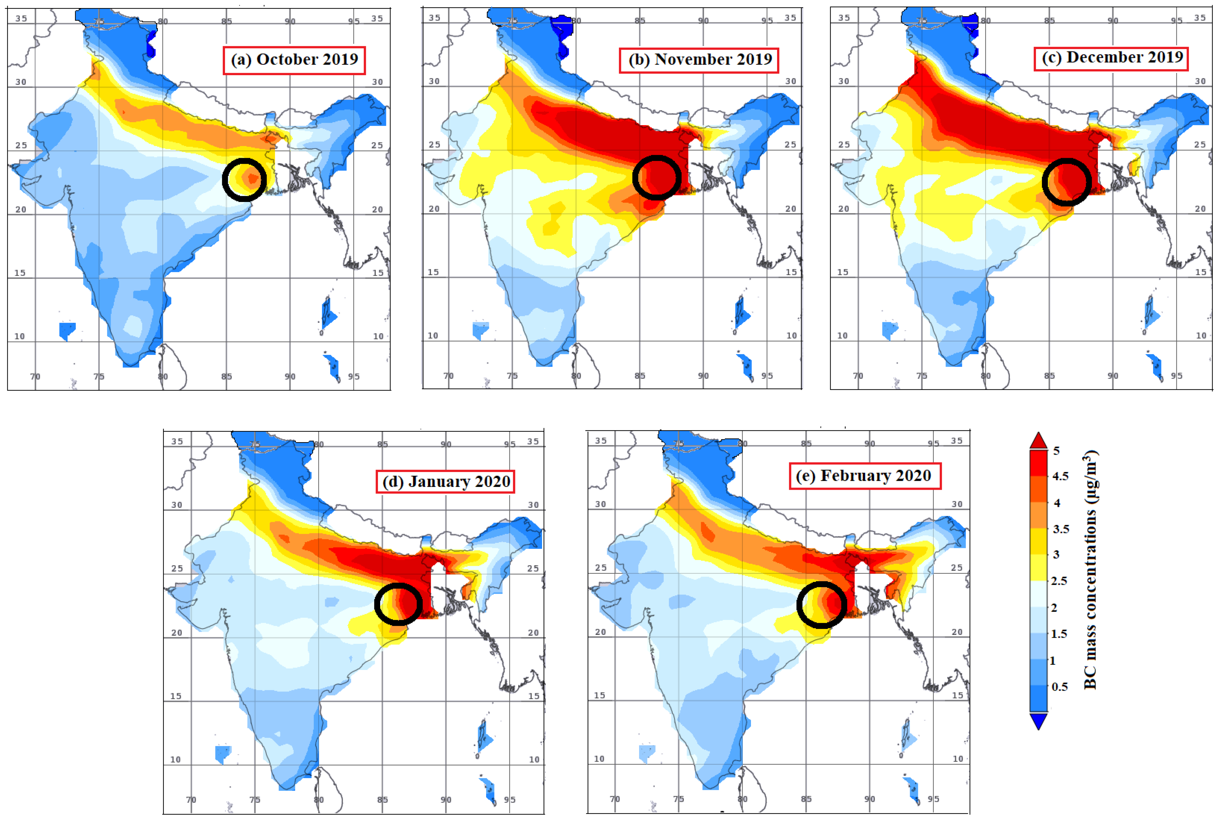
The average BC mass concentrations were recorded as 9.46 ± 3.35 μg m−3 (5.06–19.22 µg m−3) and 8.58 ± 1.60 μg m−3 (5.50–11.52 µg m−3) at JSR and KGP, respectively. The monthly mean (± standard deviation) variation of BC concentration from October 2019 to February 2020 is shown in Figure 2b. In JSR city, the monthly BC concentrations were 6.7 ± 2.05, 7.8 ± 2.10, 9.1 ± 2.67, 12.7 ± 4.1, and 11.5 ± 2.2 µg m−3, while in KGP, the BC mass concentrations were 9.5 ± 0.9, 8.4 ± 1.3, 8.9 ± 1.6, 8.0 ± 1.5, and 7.7 ± 2.0 µg m−3 in the months of October, November, December of 2019, and January and February 2020, respectively. A comparison of the average BC mass concentrations reported for various locations in India and other countries is shown in Table 2. The average BC mass concentrations at JSR (9.46 µg m−3) and KGP (8.58 µg m−3) were higher than those reported in other cities, i.e., 7.6 µg m−3 in Sao Paulo, Brazil [60], 6.64 µg m−3 in Delhi [61], 5 µg m−3 in Trivandrum [62], 4.2 µg m−3 at Bangalore [62], and 4.1 µg m−3 at Pune [63]. Lower values compared to other cities include 16.5 µg m−3 at Kharagpur [64], 35 µg m−3 and 13.5 µg m−3 at Kolkata [51], 29 µg m−3 and 13.5 µg m−3 at Delhi [51], 10.30 µg m−3 at Ahmedabad [65], and 20.6 µg m−3 at Agra [47,48]. In other cities of the world, the BC concentrations of 14.7 µg m−3 at Xi’an (China: [66]), 21.7 µg m−3 at Lahore (Pakistan: [67,68]), and 14 µg m−3 at Paris (France: [63]) were found to be higher than the 9.46 µg m−3 found at Jamshedpur and 8.58 µg m−3 at Kharagpur in the present study. Typically, at almost all sites, the BC mass concentration levels were higher in the winter season compared to other periods. In addition to higher emissions, the shallow mixing layer height (MLH) in the winter season could also be an important factor leading to higher concentrations of BC. Further, the monthly average maps of BC surface mass concentrations obtained from the MERRA-2 model (M2TMNXAER v 5.12.4) are plotted in Figure 3. The maps depict the occurrence of increased BC mass concentrations throughout the IGP, including the area of interest during the winter season. We are confident enough to employ the geographically weighted regression (GWR) PM2.5 product to corroborate the spatiotemporal distribution of MERRA-2 PM2.5. this is due to the significant correlation coefficient (R = 0.73) that demonstrated outstanding agreement between GWR PM2.5 and ground-based PM2.5.
3.2. Characteristics of Ionic Species
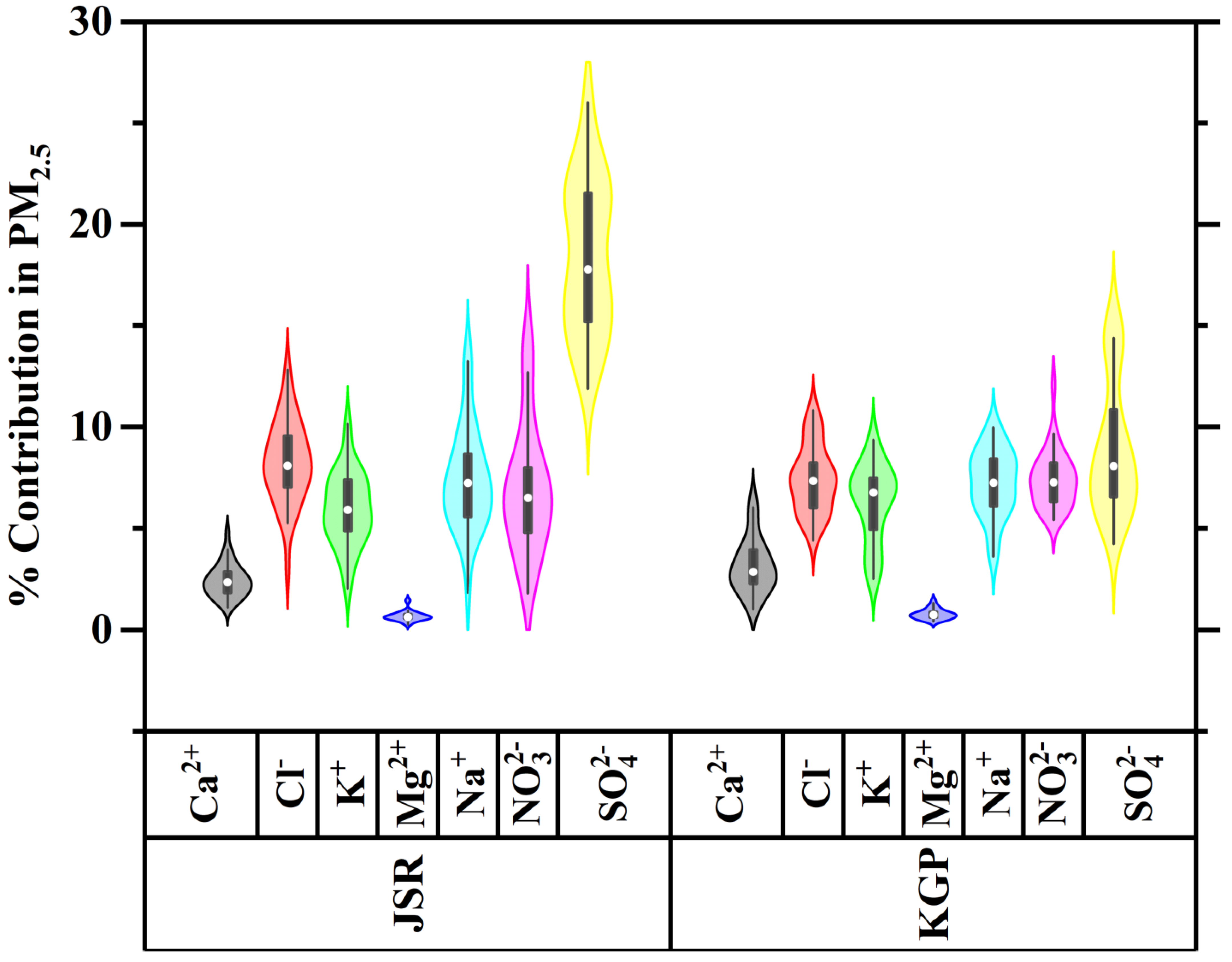
The PM2.5 aerosols have been characterized by the abundances of anions (Cl−, NO32−, SO42−) and cations (Na+, K+, Ca2+, Mg2+). A summary of the mass concentration of ionic species in PM2.5 at JSR and KGP is given in Table 3 and the violin and box plots of the percentage contribution of ionic species in PM2.5 are shown in Figure 4. The mass concentrations of significant PM2.5 ionic species are in the order of SO42− > Cl− > Na+ > NO3− > K+ > Ca2+ > Mg2+ at JSR and SO42− > NO3− > Cl− > Na+ > K+ > Ca2+ > Mg2+ at KGP. The contributions of these major ionic species to the total PM2.5 mass were found at ~33.89% (anion) and 16.62% (cation) at JSR and 23.83% (anion) and 17.61% (cation) at KGP. The Cl−/Na+ ratio varied in the ranges of 0.30–5.11 and 0.65–2.10, with average values of 1.28 and 1.08 at JSR and KGP, respectively. The ratios for the study sites differ greatly from those of ~1.8 for ocean water, indicating that the ocean salt has a relatively minor impact. A moderate correlation (~0.66) between Na+ and Cl− species indicates significant similarities in their emission sources. A recent study also reported the minor influences of ocean salt airborne in different regions of IGP during the winter season [36,39,52,57] and over Varanasi [9,58]. The ratio of Mg2+/Na+, Ca2+/Na+, SO42−/Na+, Cl−/Mg2+, and Na+/Mg2+ were 0.11, 0.41, 2.14, 11.08, and 11.29, respectively. Nonetheless, the ratios of Mg2+/Na+ and Ca2+/Na+ in the present study are found to be lesser than their ratios in the seawater, while the ratio of SO42−/Na+ was higher. At the same time, the ratios of Cl−/Mg2+ and Na+/Mg2+ are very high, indicating the major influences of anthropogenic and terrestrial emissions [69]. The non-ocean salt (nos) parts of water-soluble ions are determined by utilizing Na+ as a reference component for oceanic salt abundance [70,71]. The contributions of other ionic species such as SO42−, K+, and Ca2+ to total PM2.5 ions (measured) are found to be 36.91%, 12.14%, and 4.75% at JSR and 21.46%, 15.46%, and 7.65% at KGP, respectively. The significant sources of nos-SO42− could be coal burning, non-renewable energy sources, biomass/biofuel burning, vehicular exhaust, and SO2 oxidation in the atmosphere [72,73]. The emissions from environmental variables such as paint and cement factories that discharge multiple chemicals into the atmosphere may be the other possible causes of anions. The higher concentrations of K+ in November could be due to firecrackers during the Diwali festival celebration and extensive emissions from biomass/crop-residue burning sources. It is to be noted that the abundance of K+ has been considered an important indicator/trace for biomass burning emissions [34,74]. Likewise, [75] reported the significant role of crop residue burning (CRB) in the northern parts of India, leading to higher concentrations of fine PMs (0.1–1 μm) including BC during the post-monsoon period.
3.3. Source Apportionment of PM2.5 and BC
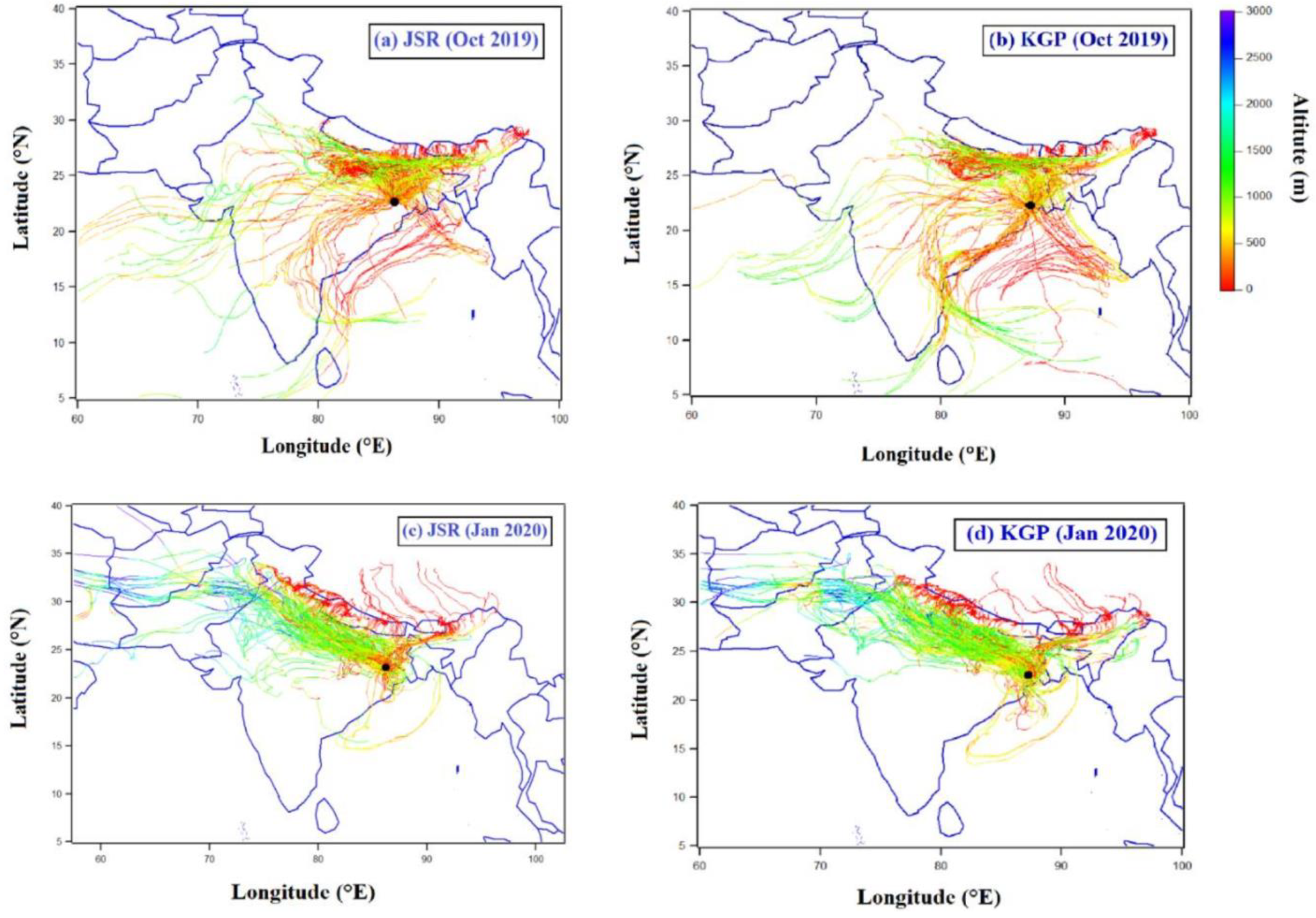
The backward trajectory analysis is widely applied to understand the source (local/regional) and transport routes of air pollutants. In this study, the trajectories were set up with the assistance of Igor programming. The input data required for the trajectory calculation was taken from the CFS and METEX created by the Center for Global Environmental Research (CGER), Japan, and the National Centers for Environmental Prediction (NCEP). The back trajectories were analyzed for both cities from east India (Figure 5). The analysis of the back trajectories suggests that air masses originated from different heights and regions. In both study locations, airborne particulate matter transport from the sources located in the north, northwest, and east can be observed in October. In addition to continental origin, the transport from marine regions of the Arabian Sea and the Bay of Bengal (BoB) seems to influence the study sites. Therefore, oceanic air masses could have contributed to salt particulate matter content during the study period. In the JSR region, the contribution of salt particulate matter is less compared to the KGP region. This is because of KGP’s location on the shore and its closeness to the coast; the meteorology shifted the wind direction from the Bay of Bengal to KGP, as did the influence of the sea breeze on the coastal districts. Regionally, transports of air masses from the neighboring states of Bihar, Utter Pradesh, Odisha, and central parts of India were prominent. Besides the air masses originating from different parts of India, the trajectories indicate the transport from different neighboring countries (Nepal, Pakistan, Bhutan, etc.) to some extent. It can also be noted that the transport from north, northwest, and northeast regions prevailed in the month of January. Most of the trajectories have been traced to the northwest during this month, including Pakistan, Afghanistan, Iran, Nepal, Bhutan, and China. The overall trajectories suggest that the most significant influences were from the IGP region.
The coal-burning sector continues to be the primary source of energy, accounting for 76% of the requirements in India, and this sector remains the main source of BC [76]. We used the ‘aethalometer model’ to investigate the primary sources of BC influencing the study sites. However, the projected model focused on a few selective sources such as wood burning and traffic emissions. Figure 6 shows how the BC differed from the city in its source distinction between wood burning and fossil fuels. The wood-burning contribution was about 36.36% for ambient BC mass concentration and the fossil fuel contribution was approximately 51.51% at JSR. At KGP, the wood-burning contribution was 43.75% and the fossil fuel contribution was 34.37% for the BC mass concentration measured during the present study.
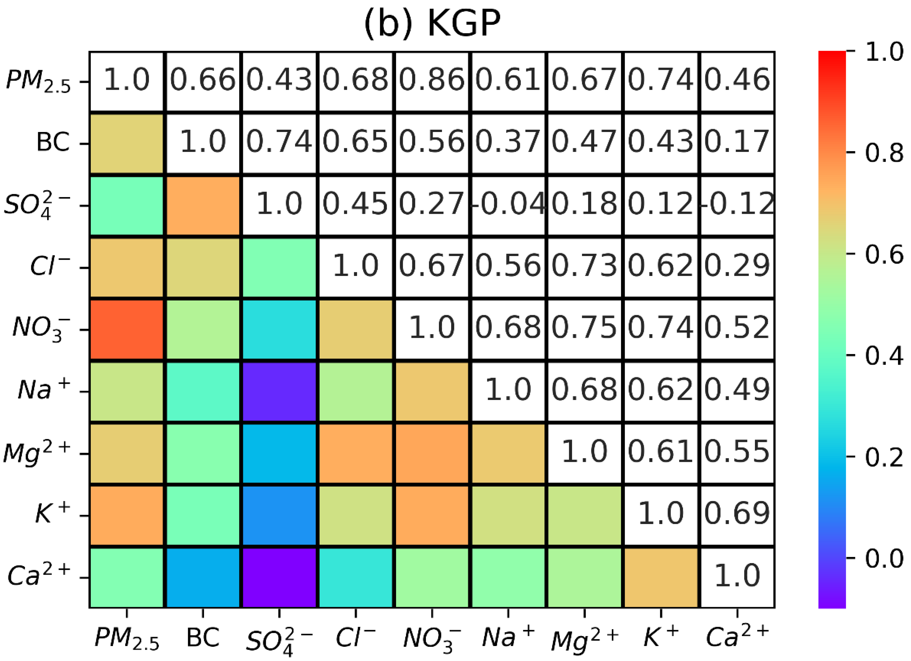
In summary, the contributions of fossil fuel-based emissions to ambient air BC mass concentration in the JSR region are higher than that in the KGP region. This is consistent with the higher volume of vehicular traffic in the JSR region than in the KGP region. The BC and PM2.5 concentrations in the JSR site were higher than those in the KGP site. As shown in Figure 6, the BC and PM2.5 concentrations showed a moderate correlation (r = 0.42) at JSR and a good positive Pearson correlation (r = 0.66) at KGP. The BC and PM2.5 concentrations were thus likely emitted from the same sources as wood burning, fossil fuel burning, coal burning, traffic emissions, construction works, etc. The present research helps policymakers and future researchers by providing the first inventory of atmospheric particulate-bound chemical concentrations and BC patterns in middle-east India.
3.4. Role of Transport Using Air Mass Back Trajectory
Investigations were carried out with the help of a 7-day HYSPLIT back-trajectory analysis for the role of transport to learn more about the cause of the disparity in magnitudes. Additionally, we looked at the impact of air mass trajectories, which serve as available paths for aerosol movement, to further investigate the connection between air mass sources and BC. The 7-day isentropic cluster mean air mass backward trajectories are shown in Figure 5. Using PC-based HYSPLIT, the variation in height (m) representing the contour was calculated at 500 m AGL across KGP and JSR. Reference [77] provides a comprehensive description of this investigation. As they account for the adiabatic vertical movements of air parcels during transit and are less subject to inaccuracies in the fundamental meteorological data, trajectories were taken into consideration. According to Figure 7, the cluster means backward trajectories over JSR exhibit almost the same pattern as those over KGP. This cluster analysis pathways throughout the campaign time were extremely evident.
4. Summary and Conclusions
In this study, the BC, PM2.5 mass concentrations, and chemical speciation of PM2.5 were measured at Jamshedpur (JSR) and Kharagpur (KGP) in the eastern part of India during the winter season. The city of JSR had a mean BC mass concentration of 9.46 ± 3.35 µg m−3, whereas KGP had an average BC mass concentration of 8.58 ± 1.60 µg m−3. JSR observed a maximum BC mass concentration of 12.71 µg m−3 in December 2019, while KGP observed a maximum of 9.56 µg m−3 in October 2019. In JSR and KGP, BC mass concentrations varied between 5.06–19.22 µg m−3 and 5.50–11.52 µg m−3, respectively. The mean PM2.5 concentration was 156.69 ± 33.62 µg m−3 at JSR and was 126.41 ± 21.78 µg m−3 at KGP. In addition to local sources, backward air trajectories showed that the transport of air masses originated mainly from the northern part of India (mainly IGP) and the neighboring countries. The diagnostic ratio analysis suggests that the BC contribution from fossil fuel (51.51%) was higher than that of wood burning (36.36%) at JSR. On the other hand, at the KGP site, the fossil fuel contribution (34.37%) is lower than that of the wood-burning contribution (43.75%). The higher contributions of BC from fossil fuels at JSR are because of more industrialization and the high traffic load. The mass of PM2.5 ionic species was in the order of SO42− > Cl− > Na+ > NO3− > K+ > Ca2+ > Mg2+ in JSR, while the order was SO42− > NO3− > Cl− > Na+ > K+ > Ca2+ > Mg2+ in KGP. The significant commitment of complete ionic species mass concentration in PM2.5 was around 33.89% (anion) and 16.62% (cation) at JSR and 23.83% (anion) and 17.61% (cation) at KGP. The masses of SO42−, K+, and Ca2+ in PM2.5 (absolute particles) are estimated to be 36.91%, 12.14%, and 4.75% at JSR and 21.46%, 15.46%, and 7.65% at KGP, respectively. The concentrations of BC and PM2.5 show a moderate positive Pearson correlation (r = 0.42) at JSR and a good positive Pearson correlation (r = 0.66) at KGP, east India, indicating similar sources of origin.
Author Contributions
The data collection and analysis, conception, and design of the study were conducted by B.A. The first draft was written by T.K.S. The data interpretation was carried out by L.K.S. Editing, interpretation, reviewing, and plotting were carried out by U.C.D. All authors have read and agreed to the published version of the manuscript.
Funding
The current work received external funding from the SERB (via letter no. ECR/2017/000597), DST, Government of India.
Institutional Review Board Statement
Not applicable in the present study.
Informed Consent Statement
Not applicable in the present study.
Data Availability Statement
The datasets developed during the current work are available from the corresponding author on reasonable request.
Acknowledgments
The authors are thankful to the Director, NIT Jamshedpur, and departmental colleagues for their encouragement and support of this study. The authors thankfully acknowledge the National Oceanic and Atmospheric Administration (NOAA) Air Resources Laboratory for downloading the air mass trajectories (http://www.arl.noaa.gov/ready/hysplit4.html) (accessed on 1 August 2022). The SERB-DST (Science and Engineering Research Board, Department of Science and Technology), Government of India, financially supported the research via letter no. ECR/2017/000597. We thank editor, and all three anonymous reviewers for their encouragement and insightful comments and valuable suggestions, which helped us to improve the scientific quality of the manuscript. We are grateful to section managing editor, for allowing us to serve as a guest editor in this special issue.
Conflicts of Interest
The authors declare that they have no conflict of interest.
References
- Sahu, L.K.; Kondo, Y.; Moteki, N.; Takegawa, N.; Zhao, Y.; Cubison, M.J.; Jimenez, J.L.; Vay, S.; Diskin, G.S.; Wisthaler, A.; et al. Emission characteristics of black carbon in anthropogenic and biomass burning plumes over California during ARCTAS-CARB 2008. J. Geophys. Res. 2012, 117, D16302. [Google Scholar] [CrossRef]
- Naudiyal, N.; Schmerbeck, J. The changing Himalayan landscape: Pine-oak forest dynamics and the supply of ecosystem services. J. For. Res. 2017, 28, 431–443. [Google Scholar] [CrossRef]
- Sahu, L.K.; Kondo, Y.; Miyazaki, Y.; Pongkiatkul, P.; Oanh, N.T.K. Seasonal and diurnal variations of black carbon and organic carbon aerosols in Bangkok. J. Geophys. Res. 2011, 116, D15302. [Google Scholar] [CrossRef]
- Pani, S.K.; Chantara, S.; Khamkaew, C.; Lee, C.T.; Lin, N.H. Biomass burning in the northern peninsular Southeast Asia: Aerosol chemical profile and potential exposure. Atmos. Res. 2019, 224, 180–195. [Google Scholar] [CrossRef]
- Gatari, M.J.; Kinney, P.L.; Yan, B.; Sclar, E.; Volavka-Close, N.; Ngo, N.S.; Gaita, S.M.; Law, A.; Nbida, P.K.; Gachanja, A.; et al. High airborne black carbon concentrations measured near roadways in Nairobi, Kenya. Transp. Res. Part Transp. Environ. 2019, 68, 99–109. [Google Scholar] [CrossRef]
- IPCC. Climate Change. In The Physical Science Basis. Working Group, I Contribution to the IPCC 5th Assessment Report; IPCC: Cambridge, UK; New York, NY, USA, 2013. [Google Scholar]
- Liu, Y.; Yan, C.; Zheng, M. Source apportionment of black carbon during winter in Beijing. Sci. Total Environ. 2018, 618, 531–541. [Google Scholar] [CrossRef]
- Joshi, H.; Naja, M.; Singh, K.P.; Kumar, R.; Bhardwaj, P.; Babu, S.S.; Satheesh, S.K.; Moorthy, K.K.; Chandola, H.C. Investigations of aerosol black carbon from a semi-urban site in the Indo-Gangetic Plain region. Atmos. Environ. 2016, 125, 346–359. [Google Scholar] [CrossRef]
- Tiwari, S.; Dumka, U.C.; Kaskaoutis, D.G.; Ram, K.; Panicker, A.S.; Srivastava, M.K.; Tiwari, S.; Attri, S.D.; Soni, V.K.; Pandey, A.K. Aerosol chemical characterization and role of carbonaceous aerosol on radiative effect over Varanasi in central indo-Gangetic plain. Atmos. Environ. 2016, 125, 437–449. [Google Scholar] [CrossRef]
- Ming, J.; Xiao, C.D.; Cachier, H.; Qin, D.H.; Qin, X.; Li, Z.Q.; Pu, J.C. Black Carbon (BC) in the snow of glaciers in west China and its potential effects on albedos. Atmos. Res. 2009, 92, 114–123. [Google Scholar] [CrossRef]
- WHO (World Health Organization). Health effects of black carbon. In Joint WHO/UNECE Task Force on Health Aspects of Air Pollutants under UNECE’s Long-Range Transboundary Air Pollution Convention (LRTAP); World Health Organization, Regional Office for Europe: Copenhagen, Denmark, 2012. [Google Scholar]
- Janssen, N.H.; Janssen, N.; Gerlofs, N.M. Health Effects of Black Carbon; World Health Organization: Copenhagen, Denmark, 2012. [Google Scholar]
- Louwies, T.; Nawrot, T.; Cox, B.; Dons, E.; Penders, J.; Provost, E.; Panis, L.I.; De Boever, P. Blood pressure changes in association with black carbon exposure in a panel of healthy adults are independent of retinal microcirculation. Environ. Int. 2015, 75, 81–86. [Google Scholar] [CrossRef]
- Li, Y.; Henze, D.K.; Jack, D.; Henderson, B.H.; Kinney, P.L. Assessing public health burden associated with exposure to ambient black carbon in the United States. Sci. Total Environ. 2016, 539, 515–525. [Google Scholar] [CrossRef]
- Lin, W.; Dai, J.; Liu, R.; Zhai, Y.; Yue, D.; Hu, Q. Integrated assessment of health risk and climate effects of black carbon in the Pearl River Delta region, China. Environ. Res. 2019, 176, 108522. [Google Scholar] [CrossRef] [PubMed]
- Wang, R.; Tao, S.; Balkanski, Y.; Ciais, P.; Boucher, O.; Liu, J.; Piao, S.; Shen, H.; Vuolo, M.R.; Valari, M.; et al. Exposure to ambient black carbon derived from a unique inventory and high-resolution model. Proc. Natl. Acad. Sci. USA 2014, 111, 2459–2463. [Google Scholar] [CrossRef] [PubMed]
- Cao, J.; Xu, H.; Xu, Q.; Chen, B.; Kan, H. Fine particulate matter constituents and cardiopulmonary mortality in a heavily polluted Chinese city. Environ. Health Perspect. 2012, 120, 373–378. [Google Scholar] [CrossRef] [PubMed]
- Atkinson, R.W.; Mills, I.C.; Walton, H.A.; Anderson, H.R. Fine particle components and health systematic review and meta-analysis of epidemiological time series studies of daily mortality and hospital admissions. J. Expo. Sci. Environ. Epidemiol. 2015, 25, 208. [Google Scholar] [CrossRef] [PubMed]
- Ohara, T.; Akimoto, H.; Kurokawa, J.; Horii, N.; Yamaji, K.; Yan, X.; Hayasaka, T. An Asian emission inventory of anthropogenic emission sources for the period 19802020. Atmos. Chem. Phys. 2007, 7, 4419–4444. [Google Scholar] [CrossRef]
- Chernyshev, V.V.; Zakharenko, A.M.; Ugay, S.M.; Hien, T.T.; Hai, L.H.; Olesik, S.M.; Kholodov, A.S.; Zubko, E.; Kokkinakis, M.; Burykina, T.I.; et al. Morphological and chemical composition of particulate matter in buses exhaust. Toxicol. Rep. 2019, 6, 120–125. [Google Scholar] [CrossRef]
- Liu, K.; Wang, F.; Li, J.; Tiwari, S.; Chen, B. Assessment of trends and emission sources of heavy metals from the soil sediments near the Bohai Bay. Environ. Sci. Pollut. R. 2019, 26, 29095–29109. [Google Scholar] [CrossRef]
- Pani, S.K.; Ou-Yang, C.F.; Wang, S.H.; Ogren, J.A.; Sheridan, P.J.; Sheu, G.R.; Lin, N.H. Relationship between long-range transported atmospheric black carbon and carbon monoxide at a high-altitude background station in East Asia. Atmos. Environ. 2019, 210, 86–99. [Google Scholar] [CrossRef]
- WHO. Burden of Disease from Ambient Air Pollution for 2012; Description of Method, Version 1.3; WHO: Geneva, Switzerland, 2014. [Google Scholar]
- WHO. WHO’s Ambient Air Pollution Database e Update 2014.Data Summary of the AAP Database; WHO: Geneva, Switzerland, 2014; Available online: http://www.who.int/phe/health_topics/outdoorair/databases/AAP_database_results_2014b (accessed on 1 August 2022).
- Tiwari, S.; Kaskaoutis, D.; Soni, V.K.; Attri, S.D.; Singh, A.K. Aerosol columnar characteristics and their heterogeneous nature over Varanasi, in the Central Ganges valley. Environ. Sci. Pollut. Res. 2018, 25, 24726–24745. [Google Scholar] [CrossRef]
- Seinfeld, J.H.; Bretherton, C.; Carslaw, K.S.; Coe, H.; DeMott, P.J.; Dunlea, E.J.; Feingold, G.; Ghan, S.; Guenther, A.B.; Kahn, R.; et al. Improving our fundamental understanding of the role of aerosol−cloud interactions in the climate system. Proc. Natl. Acad. Sci. USA 2016, 113, 5781–5790. [Google Scholar] [CrossRef] [PubMed]
- World Health Statistics. 2018. Available online: https://apps.who.int/iris/bitstream/handle/10665/272596/9789241565585-eng.pdf (accessed on 1 August 2022).
- Singh, A.; Rastogi, N.; Patel, A.; Satish, R.V.; Singh, D. Size-segregated characteristics of carbonaceous aerosols over the northwestern indo-gangetic plain: Year-round temporal behavior. Aerosol Air Qual. Res. 2016, 16, 1615–1624. [Google Scholar] [CrossRef]
- Satsangi, A.; Pachauri, T.; Singla, V.; Lakhani, A.; Kumari, K.M. Water soluble ionic species in atmospheric aerosols: Concentrations and sources at Agra in the indo-Gangetic plain (IGP). Aerosol Air Qual. Res. 2013, 13, 1877–1889. [Google Scholar] [CrossRef]
- Satsangi, P.G.; Pipal, A.S.; Budhavant, K.B.; Rao, P.S.P.; Taneja, A. Study of chemical species associated with fine particles and their secondary particle formation at semi-arid region of India. Atmos. Pollut. Res. 2016, 7, 1110–1118. [Google Scholar] [CrossRef]
- China, S.; Mazzoleni, C.; Gorkowski, K.; Aiken, A.C.; Dubey, M.K. Morphology and mixing state of individual freshly emitted wildfire carbonaceous particles. Nat. Commun. 2013, 4, 2122. [Google Scholar] [CrossRef]
- Tsai, T.C.; Jeng, Y.J.; Chu, D.A.; Chen, J.P.; Chang, S.C. Analysis of the relationship between MODIS aerosol optical depth and particulate matter from 2006 to 2008. Atmos. Environ. 2011, 45, 4777–4788. [Google Scholar] [CrossRef]
- Rajput, P.; Sarin, M.M.; Sharma, D.; Singh, D. Atmospheric polycyclic aromatic hydrocarbons and isomer ratios as tracers of biomass burning emissions in northern India. Environ. Sci. Pollut. Res. 2014, 21, 5724–5729. [Google Scholar] [CrossRef]
- Ram, K.; Sarin, M.M.; Tripathi, S.N. Temporal trends in atmospheric PM2.5, PM10, elemental carbon, organic carbon, water-soluble organic carbon, and optical properties: Impact of biomass burning emissions in the Indo-Gangetic Plain. Environ. Sci. Technol. 2012, 46, 686–695. [Google Scholar] [CrossRef]
- Roy, A.; Chatterjee, A.; Tiwari, S.; Sarkar, C.; Das, S.K.; Ghosh, S.K.; Raha, S. Precipitation chemistry over urban, rural and high-altitude Himalayan stations in eastern India. Atmos. Res. 2016, 181, 44–53. [Google Scholar] [CrossRef]
- Goel, V.; Mishra, S.K.; Ahlawat, A.; Sharma, C.; Vijayan, N.; Radhakrishnan, S.R.; Dimri, A.P.; Kotnala, R.K. Effect of reduced traffic density on characteristics of particulate matter over Delhi. Curr. Sci. 2018, 115, 315. [Google Scholar] [CrossRef]
- Verma, S.; Pani, S.K.; Bhanja, S.N. Sources and radiative effects of wintertime black carbon aerosols in an urban atmosphere in east India. Chemosphere 2013, 90, 260–269. [Google Scholar] [CrossRef] [PubMed]
- Allen, G.A.; Lawrence, J.; Koutrakis, P. Field validation of a semicontinuous method for aerosol black carbon (aethalometer) and temporal patterns of summertime hourly black carbon measurements in southwestern PA. Atmos. Environ. 1999, 33, 817–823. [Google Scholar] [CrossRef]
- Weingartner, E.; Saathoff, H.; Schnaiter, M.; Streit, N.; Bitnar, B.; Baltensperger, U. Absorption of light by soot particles, determination of the absorption coefficient by means of aethalometers. J. Aerosol Sci. 2003, 34, 1445–1463. [Google Scholar] [CrossRef]
- Fuller, G.W.; Tremper, A.H.; Baker, T.D.; Yttri, K.E.; Butterfield, D. Contribution of wood burning to PM10 in London. Atmos. Environ. 2014, 87, 87–94. [Google Scholar] [CrossRef]
- Thepnuan, D.; Chantara, S.; Lee, C.T.; Lin, N.H.; Tsai, Y.I. Molecular markers for biomass burning associated with the characterization of PM2.5 and component sources during dry season haze episodes in Upper South East Asia. Sci. Total Environ. 2019, 658, 708–722. [Google Scholar] [CrossRef]
- Zhang, Y.L.; Schnelle-Kreis, J.; Abbaszade, G.; Zimmermann, R.; Zotter, P.; Shen, R.-R.; Schäfer, K.; Shao, L.; Prévôt, A.S.H.; Szidat, S. Source apportionment of elemental carbon in Beijing, China: Insights from radiocarbon and organic marker measurements. Environ. Sci. Technol. 2015, 49, 8408–8415. [Google Scholar] [CrossRef] [PubMed]
- Favez, O.; Haddad, E.I.I.; Piot, C.; Bor_eave, A.; Abidi, E.; Marchand, N.; Jaffrezo, J.-L.; Besombes, J.-L.; Personnaz, M.B.; Sciare, J.; et al. Inter-comparison of source apportionment models for the estimation of wood burning aerosols during wintertime in an Alpine city (Grenoble, France). Atmos. Chem. Phys. 2010, 10, 5295–5314. [Google Scholar] [CrossRef]
- Larsen, B.R.; Gilardoni, S.; Stenstrom, K.; Niedzialek, J.; Jimenez, J.; Belis, C.A. Sources for PM air pollution in the Po Plain, Italy: II. Probabilistic uncertainty characterization and sensitivity analysis of secondary and primary sources. Atmos. Environ. 2012, 50, 203–213. [Google Scholar] [CrossRef]
- Briggs, N.L.; Long, C.M. Critical review of black carbon and elemental carbon source apportionment in Europe and the United States. Atmos. Environ. 2016, 144, 409–427. [Google Scholar] [CrossRef]
- Zotter, P.; Herich, H.; Gysel, M.; El-Haddad, I.; Zhang, Y.; Mo_cnik, G.; Hüglin, C.; Baltensperger, U.; Szidat, S.; Prevot, A.S.H. Evaluation of the absorption Ångstr€om exponents for traffic and wood burning in the Aethalometer-based source apportionment using radiocarbon measurements of ambient aerosol. Atmos. Chem. Phys. 2017, 17, 4229–4249. [Google Scholar] [CrossRef] [Green Version]
- Dumka, U.C.; Kaskaoutis, D.G.; Tiwari, S.; Safai, P.D.; Attri, S.D.; Soni, V.K.; Singh, N.; Mihalopoulos, N. Assessment of biomass burning and fossil fuel contribution to black carbon concentrations in Delhi during winter. Atmos. Environ. 2018, 194, 93–109. [Google Scholar] [CrossRef]
- Dumka, U.C.; Kaskaoutis, D.G.; Devara, P.C.S.; Kumar, R.; Kumar, S.; Tiwari, S.; Gerasopoulos, E.; Mihalopoulos, N. Year-long variability of the fossil fuel and wood burning black carbon components at a rural site in southern Delhi outskirts. Atmos. Res. 2019, 216, 11–25. [Google Scholar] [CrossRef]
- Wang, Y.; Hopke, P.K.; Utell, M.J. Urban-scale spatial-temporal variability of black carbon and winter residential wood combustion particles. Aerosol Air Qual. Res. 2011, 11, 473–481. [Google Scholar] [CrossRef]
- Herich, H.; Hueglin, C.; Buchmann, B.A. 2.5 year’s source apportionment study of black carbon from wood burning and fossil fuel combustion at urban and rural sites in Switzerland. Atmos. Meas. Tech. 2011, 4, 1409–1420. [Google Scholar] [CrossRef]
- Kumar, R.R.; Soni, V.K. Evaluation of spatial and temporal heterogeneity of black carbon aerosol mass concentration over India using three-year measurements from IMD BC observation network. Sci. Total Environ. 2020, 723, 138060. [Google Scholar] [CrossRef]
- Thurston, G.D.; Ito, K.; Lall, R. A source apportionment of US fine particulate matter air pollution. Atmos. Environ. 2011, 45, 3924–3936. [Google Scholar] [CrossRef]
- Tare, V.; Tripathi, S.N.; Chinnam, N.; Srivastava, A.K.; Dey, S.; Manar, M.; Kanawade, V.P.; Agarwal, A.; Kishore, S.; Lal, R.B.; et al. Measurements of atmospheric parameters during Indian Space Research Organization Geosphere Biosphere Program Land Campaign II at a typical location in the Ganga Basin: 2. Chemical properties. J. Geophys. Res. Atmos. 2006, 111, 1–14. [Google Scholar] [CrossRef]
- Murari, V.; Kumar, M.; Singh, N.; Singh, R.S.; Banerjee, T. Particulate morphology and elemental characteristics: Variability at middle Indo-Gangetic plain. J. Atmos. Chem. 2016, 73, 165–179. [Google Scholar] [CrossRef]
- Tiwari, S.; Srivastava, A.K.; Bisht, D.S.; Bano, T.; Singh, S.; Behura, S.; Srivastava, M.K.; Chate, D.M.; Padmanabhamurty, B. Black carbon and chemical characteristics of PM10 and PM2.5 at an urban site of North India. J. Atmos. Chem. 2009, 62, 193–209. [Google Scholar] [CrossRef]
- Guttikunda, S.K.; Calori, G. A GIS based emissions inventory at 1 km × 1 km spatial resolution for air pollution analysis in Delhi, India. Atmos. Environ. 2013, 67, 101–111. [Google Scholar] [CrossRef]
- Pipal, A.S.; Jan, R.; Satsangi, P.G.; Tiwari, S.; Taneja, A. Study of surface morphology, elemental composition and origin of atmospheric aerosols (PM2.5 and PM10) over Agra, India. Aerosol Air Qual. Res. 2014, 14, 1685–1700. [Google Scholar] [CrossRef]
- Sen, A.; Abdelmaksoud, A.S.; Ahammed, Y.N.; Banerjee, T.; Bhat, M.A.; Chatterjee, A.; Choudhuri, A.K.; Das, T.; Dhir, A.; Dhyani, P.P.; et al. Variations in particulate matter over indo-Gangetic Plains and indo-Himalayan range during four field campaigns in winter monsoon and summer monsoon: Role of pollution pathways. Atmos. Environ. 2017, 154, 200–224. [Google Scholar] [CrossRef]
- Pratap, V.; Kumar, A.; Tiwari, S.; Kumar, P.; Tripathi, A.K.; Singh, A.K. Chemical characteristics of particulate matters and their emission sources over Varanasi during winter season. J. Atmos. Chem. 2020, 77, 83. [Google Scholar] [CrossRef]
- Castanho, A.D.A.; Artaxo, P. Wintertime and summertime Sao Paulo aerosol source apportionment study. Atmos. Environ. 2001, 35, 4889–4902. [Google Scholar] [CrossRef]
- Tiwari, S.; Srivastava, A.K.; Bisht, D.S.; Parmita, P.; Srivastava, M.K.; Attri, S.D. Diurnal and seasonal variation of black carbon and PM2.5 over New Delhi, India: Influence of meteorology. Atmos. Res. 2013, 125–126, 50–62. [Google Scholar] [CrossRef]
- Babu, S.S.; Moorthy, K.K. Aerosol black carbon over a tropical station in India. Geophys. Res. Lett. 2002, 29, 2098. [Google Scholar] [CrossRef]
- Safai, P.D.; Kevat, S.; Praveen, P.S.; Rao, P.S.P.; Momin, G.A.; Ali, K.; Devara, P.C.S. Seasonal variation of black carbon aerosols over a tropical urban city of Pune, India. Atmos. Environ. 2007, 41, 2699–2709. [Google Scholar] [CrossRef]
- Nair, V. Wintertime aerosol characteristics over the Indo-Gangetic plain (IGP): Impacts of local boundary layer processes and long-range transport. J. Geophys. Res. 2007, 112, D13205. [Google Scholar] [CrossRef]
- Rajesh, T.A.; Ramachandran, S. Black carbon aerosols over urban and high-altitude remote regions: Characteristics and radiative implications. Atmos. Environ. 2018, 194, 110–122. [Google Scholar] [CrossRef]
- Cao, J.J.; Zhu, C.S.; Chow, J.C.; Watson, J.G.; Han, Y.M.; Wang, G.H.; Shen, Z.X.; An, Z.S. Black carbon relationships with emissions and meteorology in Xi’an, China. Atmos. Res. 2009, 94, 194–202. [Google Scholar] [CrossRef]
- Bilal, M.; Mhawish, A.; Nichol, J.E.; Qiu, Z.; Nazeer, M.; Ali, M.A.; de Leeuw, G.; Levy, R.C.; Wang, Y.; Chen, Y.; et al. Air pollution scenario over Pakistan: Characterization and ranking of extremely polluted cities using long-term concentrations of aerosols and trace gases. Remote Sens. Environ. 2021, 264, 112617. [Google Scholar] [CrossRef]
- Bilal, M.; Ali, M.A.; Nichol, J.E.; Bleiweiss, M.P.; de Leeuw, G.; Mhawish, A.; Shi, Y.; Mazhar, U.; Mehmood, T.; Kim, J.; et al. AEROsol generic classification using a novel Satellite remote sensing Approach (AEROSA). Front. Environ. Sci. 2022, 10, 981522. [Google Scholar] [CrossRef]
- Duce, R.A.; Arimoto, R.; Ray, B.J.; Unni, C.K.; Harder, P.J. Atmospheric trace elements at Enewetak Atoll: 1. Concentrations, sources, and temporal variability. J. Geophys. Res. Ocean. 1983, 88, 5321–5342. [Google Scholar] [CrossRef]
- Sharma, S.K.; Datta, A.; Saud, T.; Saxena, M.; Mandal, T.K.; Ahammed, Y.N.; Arya, B.C. Seasonal variability of ambient NH3, NO, NO2 and SO2 over Delhi. J. Environ. Sci. 2010, 22, 1023–1028. [Google Scholar] [CrossRef]
- Ram, K.; Sarin, M.M.; Tripathi, S.N. A 1 year record of carbonaceous aerosols from an urban site in the Indo Gangetic Plain: Characterization, sources, and temporal variability. J. Geophys. Res. Atmos. 2010, 115. [Google Scholar] [CrossRef]
- Rajput, P.; Gupta, T.; Kumar, A. The diurnal variability of sulfate and nitrate aerosols during wintertime in the indo-Gangetic plain: Implications for heterogeneous phase chemistry. RSC Adv. 2016, 6, 89879–89887. [Google Scholar] [CrossRef]
- Sarkar, S.; Singh, R.P.; Chauhan, A. Crop residue burning in northern India: Increasing threat to greater India. J. Geophys. Res. Atmos. 2018, 123, 6920–6934. [Google Scholar] [CrossRef]
- Kistler, R.; Kalnay, E.; Collins, W.; Saha, S.; White, G.; Woollen, J.; Chelliah, M.; Ebisuzaki, W.; Kanamitsu, M.; Kousky, V.; et al. The NCEP/NCAR 50-Year Reanalysis. 1999. Available online: http://metosrv2.umd.edu/ekalnay/Reanalysis%20paper/REANCLOS1.html (accessed on 1 June 2022).
- SAFAR (System for Air Quality Forecasting and Research). A Special Report Emission Inventory for National Capital Region Delhi Ministry of Earth Sciences. Government of India. 2010. Available online: http://safar.tropmet.res.in (accessed on 1 June 2022).
- Lee, B.K.; Hieu, N.T. Seasonal ion characteristics of fine and coarse particles from an urban residential area in a typical industrial city. Atmos. Res. 2013, 122, 362–377. [Google Scholar] [CrossRef]
- Ganguly, D.; Jayaraman, A.; Rajesh, T.A.; Gadhavi, H. Wintertime aerosol properties during foggy and no foggy days over urban center Delhi and their implications for shortwave radiative forcing. J. Geophys. Res. 2006, 111, D15217. [Google Scholar] [CrossRef] [Green Version]
Figure 1.
Locations of JSR and KGP observation sites and surrounding regions (courtesy google map; assessed on 1 August 2022).
Figure 1.
Locations of JSR and KGP observation sites and surrounding regions (courtesy google map; assessed on 1 August 2022).

Figure 2.
Monthly (average ± standard deviation) mass concentrations of (a) BC and (b) PM2.5 from October 2019 to February 2020 at JSR and KGP observation sites.
Figure 2.
Monthly (average ± standard deviation) mass concentrations of (a) BC and (b) PM2.5 from October 2019 to February 2020 at JSR and KGP observation sites.

Figure 3.
Time average maps of monthly BC surface mass concentration (µg/m3) for (a–e) (0.5 × 0.625 deg., MERRA-2 model M2TMNXAER v 5.12.4).
Figure 3.
Time average maps of monthly BC surface mass concentration (µg/m3) for (a–e) (0.5 × 0.625 deg., MERRA-2 model M2TMNXAER v 5.12.4).

Figure 4.
Percentage contributions of major ions in PM2.5 mass at JSR and KGP sites.

Figure 5.
Fractional contribution of BC measured at 370 and 880 nm at (a,b) sites. (Green—wood burning; pink—fossil fuel combustion; blue—mixed fuel burning).
Figure 5.
Fractional contribution of BC measured at 370 and 880 nm at (a,b) sites. (Green—wood burning; pink—fossil fuel combustion; blue—mixed fuel burning).

Figure 6.
Scatterplots of the BC versus PM2.5 concentrations at (a,b) sites.


Figure 7.
Seven-day air mass back trajectories over JSR and KGP sites starting at 500 m from ground level.
Figure 7.
Seven-day air mass back trajectories over JSR and KGP sites starting at 500 m from ground level.


Table 1.
Comparison of PM2.5 mass concentration observed in this study with previous studies conducted in Indian cities.
Table 1.
Comparison of PM2.5 mass concentration observed in this study with previous studies conducted in Indian cities.
| Sites | Type | PM2.5 (µg m−3) | Sampling Period | References |
|---|---|---|---|---|
| Kanpur | Urban | 203 ± 40 | December 2004 | [53] |
| Delhi | Urban | 232 ± 131 | January–December 2007 | [55] |
| Raipur | Semi-urban | 150.9 ± 75.6 | July 2009–June 2010 | [55] |
| Chennai | Urban | 73 | January–February 2008 | |
| Delhi | Urban | 123 ± 87 | 2008–2011 | [56] |
| Agra | Semi-urban | 121.2 | 2010–2011 | [57] |
| Varanasi | Semi-urban | 81.78 ± 66.4 | January–December 2014 | [54] |
| Darjeeling | Hilly area | 24.3 ± 13.5 | Winter 2015 | [58] |
| Lucknow | Urban | 130 ± 73 | Winter 2015 | [58] |
| Kashmir | Hilly area | 20.3 ± 13.1 | Winter 2015 | [58] |
| Kullu | Hilly area | 30.8 ± 17.2 | Winter 2015 | [58] |
| Delhi | Urban | 125.7 ± 56.6 | Winter 2015 | [58] |
| Varanasi | Semi-urban | 134 ± 48 | November 2016–February 2017 | [59] |
| Jamshedpur | Urban | 131 ± 58 | October 2019–February 2020 | Present study |
| Kharagpur | Semi-urban | 117 ± 79 | October 2019–February 2020 | Present study |
Table 2.
Comparison of BC mass concentration (µg m−3) measured at various locations in India and other countries.
Table 2.
Comparison of BC mass concentration (µg m−3) measured at various locations in India and other countries.
| Place | Location | Period | BC (µg m−3) | Reference |
|---|---|---|---|---|
| Sao Paulo, Brazil | Urban | July to September 1997 | 7.6 | [60] |
| Paris, France | Urban | August to October 1997 | 14 | [63] |
| Bangalore, India | Urban | November 2001 | 4.2 | [62] |
| Trivandrum, India | Urban Costal | August 2000 to October 2001 | 5 | [62] |
| Delhi, India | Urban | December 2004 | 29 | [60] |
| Kharagpur, India | Semi-urban | December 2004 | 16.5 | [64] |
| Agra, India | Urban | December 2004 | 20.6 | |
| Pune, India | Urban | January to December 2005 | 4.1 | [63] |
| Lahore, Pakistan | Urban | November 2005 to January 2006 | 21.7 | [65] |
| Xi’an, China | Urban | September 2003 to August 2005 | 14.7 | [66] |
| Kolkata, India | Urban | December 2009–10 | 35 | [37] |
| Delhi, India | Urban | January to December 2011 | 6.64 | [61] |
| Ahmedabad, India | Urban | January 2014 to December 2015 | 10.30 | [65] |
| Kolkata, India | Urban | 2016 to 2018 | 12.08 | [51] |
| Delhi, India | Urban | 2016 to 2018 | 13.57 | [51] |
| Jamshedpur, India | Urban | October 2019 to February 2020 | 9.46 | Present study |
| Kharagpur, India | Semi-urban | October 2019 to February 2020 | 8.58 | Present study |
Table 3.
Statistical analysis of major ionic species concentration (µg/m3) in PM2.5.
| Species | JSR | KGP | ||||||
|---|---|---|---|---|---|---|---|---|
| Min | Max | Average | SD | Min | Max | Average | SD | |
| SO42− | 14.19 | 46.21 | 29.22 | 9.52 | 4.16 | 20.72 | 11.24 | 4.35 |
| Cl− | 4.89 | 23.66 | 13.17 | 4.93 | 4.89 | 17.13 | 9.42 | 2.85 |
| NO32− | 3.29 | 26.58 | 10.72 | 5.36 | 5.10 | 17.16 | 9.46 | 2.93 |
| Na+ | 2.67 | 24.89 | 11.63 | 4.93 | 3.98 | 16.00 | 9.16 | 2.62 |
| Mg2+ | 0.26 | 2.06 | 1.05 | 0.41 | 0.43 | 2.11 | 0.99 | 0.43 |
| K+ | 2.98 | 18.14 | 9.61 | 4.19 | 2.89 | 13.21 | 8.10 | 3.08 |
| Ca2+ | 1.08 | 6.38 | 3.76 | 1.32 | 1.09 | 8.16 | 4.01 | 1.83 |
Publisher’s Note: MDPI stays neutral with regard to jurisdictional claims in published maps and institutional affiliations. |
© 2022 by the authors. Licensee MDPI, Basel, Switzerland. This article is an open access article distributed under the terms and conditions of the Creative Commons Attribution (CC BY) license (https://creativecommons.org/licenses/by/4.0/).
Share and Cite
MDPI and ACS Style
Ambade, B.; Sankar, T.K.; Sahu, L.K.; Dumka, U.C. Understanding Sources and Composition of Black Carbon and PM2.5 in Urban Environments in East India. Urban Sci. 2022, 6, 60. https://doi.org/10.3390/urbansci6030060
AMA Style
Ambade B, Sankar TK, Sahu LK, Dumka UC. Understanding Sources and Composition of Black Carbon and PM2.5 in Urban Environments in East India. Urban Science. 2022; 6(3):60. https://doi.org/10.3390/urbansci6030060
Chicago/Turabian StyleAmbade, Balram, Tapan Kumar Sankar, Lokesh K. Sahu, and Umesh Chandra Dumka. 2022. "Understanding Sources and Composition of Black Carbon and PM2.5 in Urban Environments in East India" Urban Science 6, no. 3: 60. https://doi.org/10.3390/urbansci6030060