
Development of a Heat Index Related to Air Quality and Meteorology for an Assessment of Work Performance in Thailand’s Urban Areas

1
School of Allied Health Science, University of Phayao, Phayao 56000, Thailand
2
School of Energy and Environment, University of Phayao, Phayao 56000, Thailand
3
Atmospheric Pollution and Climate Research Unit, School of Energy and Environment, University of Phayao, Phayao 56000, Thailand
*
Author to whom correspondence should be addressed.
Urban Sci. 2023, 7(4), 124; https://doi.org/10.3390/urbansci7040124
Submission received: 1 November 2023
/
Revised: 13 December 2023
/
Accepted: 13 December 2023
/
Published: 15 December 2023
Abstract
:A heat index is a key indicator directly related to meteorological factors influencing human health, particularly work performance. However, the interaction between air quality, meteorology, heat, and associated work performance is loosely defined, especially in urban areas. In this study, we develop a heat index (HI) related to air quality terms, including PM2.5, NOx, and CO, and meteorology terms, including temperature and relative humidity, to assess work performance in Thailand’s urban areas, including Chiang Mai, Bangkok, Nakhon Ratchasima, and Ubon Ratchathani, using a multivariate regression model. The regression models’ performance shows high R2 values ranging from 0.82 to 0.97, indicating a good level of performance. A recurring trend across all locations is elevated HI values during April and May, signifying typical pre-monsoon conditions in tropical regions. Following this peak, the values of the heat index (HI) begin to fall, possibly due to the start of the wet season. As shown by the decrease in productivity during periods of elevated heat index values, the observed increase in temperatures has noticeable effects on work performance.
1. Introduction
A considerable proportion of laborers employed in the construction, agriculture, and resource industries must endure extended working hours in thermally challenging circumstances in many places throughout the world [1]. According to Lundgren et al. [1], the presence of thermal stress in the workplace is associated with inherent risks and impacts. Heat-related illness comprises a wide range of conditions, including cramps due to heat and exhaustion from heat, as well as heat stroke, a rare but dangerous phenomenon [2]. To reach optimal productivity while guaranteeing worker well-being and safety, environmental hygienists and security officers must have a simple, resilient, and dependable metric for determining the level of stress generated by the thermal environment. In promoting the implementation of this metric, clear criteria must be provided [3]. Employees, particularly those who work outside or in surroundings without air conditioning, such as in the construction, agriculture, and industrial sectors, are especially vulnerable to poor conditions [3].
A heat index (HI) [4] is a key indicator that incorporates temperature and humidity to assess human temperature experience. This statistic emphasizes the significance of its influence on health and overall well-being. Many studies have been conducted to investigate the consequences of heat stress using heat indices, which are generally based on temperature and humidity [5,6,7]. However, it is important to recognize that humidity plays a significant role in the discomfort experienced during hot weather and should be carefully considered when calculating a heat stress index, particularly in tropical climate regions [8,9,10]. A variety of approaches are used to assess and evaluate heat stress, each of which is dependent on different environmental and meteorological characteristics. Several indicators, such as the National Weather Service Heat Index and Humidex, take temperature and moisture into account. Furthermore, numerous metrics, including the wet bulb globe temperature (WBGT) [11] and the Environmental Stress Index [12], take solar radiation into account. In the field of environmental health research, the Steadman apparent temperature is frequently used as a thermal index [12]. Steadman [4] proposed a heat index (HI), a statistic that integrates temperature and relative humidity to assess the perceived warmth of humans. This statistic is critical in determining the potential negative effects of this factor on human health and general welfare. Koteswara Rao et al. [13] demonstrated a link between thermal comfort and working performance. Their findings show a negative relationship between temperature and work performance, with an increase in temperature leading to a fall in job performance. Vaneckova et al. [14] investigated the link between temperature and heat index (HI) values in several areas. The results show that there is little variation in temperature and HI values throughout these locations. Furthermore, when comparing HI with temperature exposure, the sensitivity of estimates of the influence of heat on health did not show any significant differences. Anderson and Bell [15] discovered that an increase in the severity or duration of heatwaves relates to a higher risk of death.
While an HI is mostly related to temperature and relative humidity, these factors, on the other hand, have a significant and reciprocal influence on air quality [16]. High HI values, compounded with poor air quality, have the potential to increase the occurrence of heat-related illnesses and possibly mortality [17]. A previous study thoroughly investigated the delicate interaction between air quality, weather conditions, and heat, as well as their aggregate impact on occupational productivity and an increase in heat-related mortality [18]. Seinfeld and Pandis [16] highlighted the reciprocal connection between meteorological parameters and air quality, emphasizing the mutual influence of elements such as temperature, humidity, and pollutant presence. High temperatures and poor air quality, according to Kjellstrom et al. [19], have the potential to lower labor productivity, increase fatigue, and impair cognitive processes. The increase in industrial operations, as well as the increasing number of automobiles on the road, has had a substantial impact on the deterioration of air quality [20]. Furthermore, the interaction of air quality, meteorological conditions, and the consequent HI can have a significant impact on occupational productivity, especially in cities. As previously mentioned, the relationship between air quality and meteorology is intricate and is commonly used to derive an HI. However, there has been limited study on the relationship between air quality, meteorology, and HI values, as well as their impact on work performance in metropolitan regions. Thailand’s metropolitan areas have experienced a decrease in air quality, which has been attributed mostly to industrial expansion, increased emissions from automobiles, and human activities [21]. In Thailand, rising levels of air pollutants have generated public nervousness, prompting calls for immediate action [22]. In this context, air quality terms should be considered when estimating heat indices. The purpose of this study is to investigate the relationship between air quality, meteorological conditions, and the heat index in Thailand’s urban areas. We intend to investigate how these elements interact to affect work performance, with a special emphasis on the previously unknown aspect of air quality in heat index estimation.
2. Materials and Methods
2.1. General Information of Cities in This Study
We chose four cities with the highest population numbers for this study: Bangkok (5.49 million), Chiang Mai (1.79 million), Ubon Ratchathani (1.87 million), and Nakhon Ratchasima (2.63 million). Bangkok, as the core of Thailand’s political, economic, and cultural endeavors, attracts significant numbers of people from rural areas who want to improve their job chances, obtain access to education, and embrace a modern lifestyle. However, it is critical to recognize that a huge demographic shift is now taking place. Thailand is currently undergoing a demographic change marked by an increase in the proportion of elderly adults and a decline in the younger population. The demographic changes under consideration have significant ramifications for the nation’s socioeconomic environment, as well as its prospects in areas such as healthcare, labor market participation, and social welfare. Thailand’s cities exhibit a wide range of environmental and meteorological circumstances, as well as hosting a wide range of socioeconomic activities. Bangkok is an important economic center, whereas Chiang Mai is well-known for its cultural value and tourist attractiveness. Nakhon Ratchasima is an important economic hub in the northeastern region, while Ubon Ratchathani is an important facilitator of cross-border trade and regional linkages.
2.2. Multivariate Regression Models
A multivariate regression model was used in this work to analyze the complex interaction between air quality, meteorology, and HI [23]. The link between the heat index (HI) and many meteorological parameters such as temperature and relative humidity, as well as air quality indicators such as PM2.5, NOx, and CO, is investigated in this study. The following multivariate regression model was used in the analysis:
where β0 is the intercept; β1, β2, β3, β4, and β5 are the coefficients for PM2.5, CO, NOx, temperature, and relative humidity, respectively; and ε represents the error term.
HI = β0 + β1(PM2.5) + β2(CO) + β3(NOx) + β4(Temperature) + β5(Relative Humidity) + ε,
The current study made use of measurement data obtained from Thailand’s Pollution Control Department (PCD). We focused on several metropolitan areas that have been chosen as case studies. These places include Bangkok’s Meteorological Station, Chiang Mai’s Yupparaj School, Nakhon Ratchasima’s Electric Power Water Pump Station, and Ubon Ratchathani’s OTOP Center. Data from numerous locations were collected, including hourly measurements of carbon monoxide (CO), nitrogen oxides (NOx), temperature, relative humidity, and mass concentrations of particulate matter with a diameter less than 2.5 μm (PM2.5), as well as meteorological data such as temperature and relative humidity. According to Amnuaylojaroen et al. [24], the United States Environmental Protection Agency’s (EPA) criteria served as the basis for the QA/QC procedures undertaken in this investigation. The sampling goal was to collect quantifiable data on both PM2.5 exposure and microenvironmental concentrations. The quality assurance (QA) was founded on the following fundamental principles: (1) meticulous planning, testing, and execution of all procedures in strict accordance with approved standard operating procedures (SOPs) under the supervision of the study director; (2) complete traceability of all data generated; and (3) diligent documentation of any deviations or anomalies encountered during the process. Missing data in PCD measurements arose frequently, with a frequency of 15% [24,25].
In this study, we also used time series forecasting to estimate missing data points due to the time-dependent nature of our environmental data and the presence of incomplete observations. The AutoRegressive Integrated Moving Average (ARIMA) model was used in this investigation. This statistical technique is well-known for its ability to estimate future values within a dataset based on its own previous values [26]. Prior to deployment, the data were sorted chronologically and submitted to a stationarity check to determine the model’s applicability [27]. Differentiation was used in circumstances when the data were non-stationary to achieve a stationary series. Model parameters such as differencing order, autoregressive term order, and moving average term were identified using autocorrelation function (ACF) and partial autocorrelation function (PACF) plots [28]. Following the identification of the necessary parameters, the ARIMA model was trained using the available data points and then used to anticipate the intervals with missing data. The use of imputed values provided by the ARIMA model aided in the production of a comprehensive dataset, allowing for more rigorous studies and the formation of more solid conclusions. When applying the ARIMA model to analyze time series data, such as the PM2.5 datasets of Chiang Mai, crucial steps are taken to ensure the precision and dependability of the model. Firstly, it is crucial to deal with any missing values in the data through exploratory data analysis (EDA). The existence of missing values in a dataset containing 338 data points can adversely affect the performance of the model, as ARIMA requires uninterrupted data points for precise forecasting. The PM2.5 data were subjected to an Augmented Dickey–Fuller (ADF) test to assess their stationarity. The ADF statistic was calculated to be −6.7403, with a corresponding p-value of around 3.13 × 10⁻⁹. The numbers provided suggest that the PM2.5 time series is stationary, which is a crucial requirement of ARIMA modeling. After conducting an examination of the ACF and Partial Autocorrelation Function (PACF), it was suggested to use an initial ARIMA model with an order of (1,0,0). This model incorporates a single autoregressive term (p = 1) while excluding differencing (d = 0) and moving average elements (q = 0). This implies that the model is straightforward but has the potential to be successful when used in analyzing the time series data. Subsequent stages of the analysis entail applying the ARIMA (1, 0, 0) model to the PM2.5 data and performing diagnostic evaluations to gauge the model’s effectiveness and appropriateness. Ultimately, the model that was adjusted to predict PM2.5 levels was utilized to analyze air quality patterns.
2.3. Heat Index and Decrements in Work Performance
In this study, the heat stress was calculated using the Steadman Heat Index [4] to derive a generic HI that could be compared with the HI derived from a multivariate regression model. The HI was calculated by combining relative humidity and temperature, as defined by Rothfusz [29], via the following formula:
where HI is the heat index (in °C), T is the air temperature (in °C), RH is the relative humidity (percentage value between 0 and 100), c1 = −8.78, c2 = 1.61, c3 = 2.33, c4 = −0.14, c5 = −0.012, c6 = −0.016, c7 = 0.002, c8 = 0.0007, and c9 = −0.000003. Table 1 shows the health effect-based categories of HI values.
HI = c1 + c2 (T) + c3 (RH) + c4 (T)(RH) + c5 (T2) + c6 (RH2) + c7 (T2)(RH) + c8 (T)(RH2)
+ c9 (T2)(RH2).
We chose to use the heat index (HI) rather than temperature measurements in our heat health research because heat stress is thought to be a more robust signal in this setting. As a result, the following equation was used to approximate the drop in work performance, as follows [30]:
where P is the reduction in work performance (%) and HI is the heat index (°C).
P (%) = 2 × (HI, °C) − 50
3. Results
3.1. Descriptive Analysis of Air Quality and Meteorology
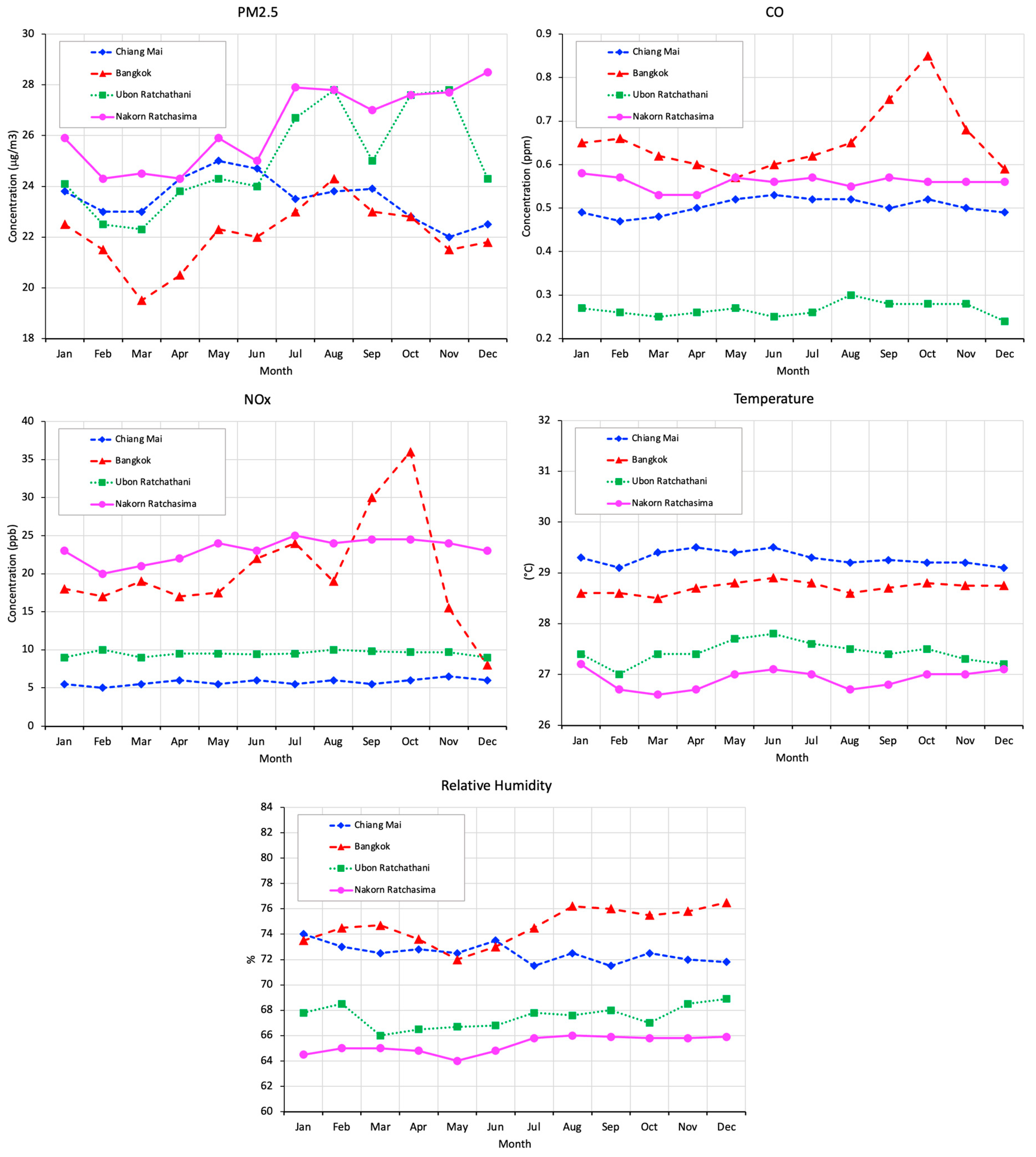
We created a plot of the seasonal variation in monthly PM2.5, CO, NOx, temperature, and relative humidity in different locations as shown in Figure 1. It compares the monthly means of five crucial environmental variables obtained from ground-based observations by the Pollution Control Department (PCD) in four provinces, including Chiang Mai, Ubon Ratchathani, Bangkok, and Nakhon Ratchasima, for CO, NOx, PM2.5, temperature, and relative humidity. The level of CO concentration in Chiang Mai province rises from January to March, reaching a peak in February. While CO levels in Ubon Ratchathani and Nakhon Ratchasima are rather steady throughout the year, the city of Chiang Mai shows an increase in NOx concentrations during the months of February and March, which corresponds to an increase in CO levels. Both Ubon Ratchathani and Nakhon Ratchasima have relatively stable NOx levels throughout the year, with a slight rise noticed in Nakhon Ratchasima near the end of the year. Meanwhile, both CO and NOx levels are significantly elevated in Bangkok in October. In terms of temperature, the annual temperature steadily rises beginning in January, peaks in either April or May, and then gradually lowers until the end of the year. Chiang Mai has a slightly lower temperature than the other provinces throughout the middle months of the year. Chiang Mai’s humidity drops in the early months, corresponding to the dry season, before increasing in the middle of the year, corresponding to the wet season (May–October). Throughout the mid-year period, Ubon Ratchathani and Nakhon Ratchasima have high relative humidity levels, which may coincide with the start of the wet season. PM2.5 concentrations in Chiang Mai rise considerably during the first few months of the year, notably around February. PM2.5 concentrations in Ubon Ratchathani and Nakhon Ratchasima are mainly constant throughout the year, with occasional increases.
Table 2 summarizes descriptive data as well as environmental and air quality observations for four Thai cities: Chiang Mai, Bangkok, Nakhon Ratchasima, and Ubon Ratchathani. In terms of overall air quality, Chiang Mai has the highest mean concentration of PM2.5 at 23.84 mg/m3. The primary cause of air pollution is most likely open burning to prepare for the planting season [20]. Bangkok has the highest mean CO concentration by 0.81 ppm. High CO levels can be attributed to the presence of urban traffic and industrial activity [31]. Nakhon Ratchasima has the highest mean NOx concentration at 35.18 ppb. This finding could suggest the presence of major contaminants in the city derived from industrial and transportation sources [32]. While air quality in Ubon Ratchathani is better than in other provinces, with PM2.5, CO, and NOx concentrations of 27.45 mg/m3, 0.27 ppm, and 9.42 ppb, respectively, Chiang Mai and Nakhon Ratchasima have higher temperature fluctuations, with standard deviations of 4.67 and 4.14, respectively. Bangkok has the highest mean relative humidity at 75.04%, while Chiang Mai has the lowest relative humidity at 53%. Also, Chiang Mai has the highest relative humidity variability, with a standard deviation of 21.84%.
3.2. Relationship between Heat Index, Air Pollutant, and Meteorology
We created the correlation plots in Figure 2 that enable a comparison of the linear correlations between major air quality and meteorological elements in four different provinces, including Chiang Mai, Ubon Ratchathani, Bangkok, and Nakhon Ratchasima. In Chiang Mai province, it is observed that the heat index increases with the increase in temperature. The correlation between PM2.5 and CO is moderately positive, with a coefficient of 0.58. Similarly, the correlation between PM2.5 and NOx is moderately positive, with a coefficient of 0.34. The correlation between relative humidity and temperature is moderately negative, with a value of −0.57. In Ubon Ratchathani province, there is a very positive correlation of 0.89 between the HI and temperature and a strong negative correlation of −0.59 between the HI and relative humidity. The relationship between PM2.5 and CO is strongly positive, with a correlation coefficient of 0.67. CO and NOx have a modest positive correlation of 0.57. In Bangkok, there is a significant positive correlation of 0.79 between the HI and temperature. However, there are moderate negative correlations of −0.42 with CO and −0.41 with NOx. PM2.5 exhibits a highly significant positive association with CO at a coefficient of 0.79 and a moderately significant positive correlation with NOx at a coefficient of 0.52. The temperature and relative humidity have a strong negative correlation of −0.65. In Nakhon Ratchasima province, the HI exhibits a highly positive correlation of 0.88 with temperature and a strong negative correlation of −0.68 with relative humidity, which aligns with similar findings in other provinces. PM2.5 exhibits a modest positive correlation with CO at a coefficient of 0.61 and with NOx at a coefficient of 0.4. As seen in other places, there is a significant inverse relationship between temperature and relative humidity, with a correlation coefficient of −0.62. Across all provinces, the HI has a strong positive relationship with temperature. This result implies that there is a positive relationship between rising temperatures and rising felt-heat indices. Furthermore, there is a minor inverse relationship between the HI and relative humidity in all provinces, showing that rising humidity levels may partially limit the increase in the heat index. There is a negative relationship between temperature and relative humidity. This finding is a common meteorological occurrence that can be attributed to a variety of factors, including dew point temperatures and the decreased moisture-holding capacity of air, which tends to increase as temperatures rise [24].
We examined the performance in estimating an HI that integrates air quality terms including PM2.5, CO, and NOx with meteorological factors such as temperature and relative humidity is illustrated via the scatter plot in Figure 3 and the statistical analysis in Table 3. As described above, the relationship between air quality, meteorology, and HI is not linearly correlated; the results of the applied multivariate regression are shown in Table 3. Table 3 presents a comprehensive examination of the intricate linkages between many environmental variables and the HI in the four provinces. It summarizes the performance measures for multivariate regression models compared to the general estimation of HI. Several factors were included in the models, including PM2.5, CO, NOx, temperature, and relative humidity. In general, the results show that the regression models for each of the four provinces function effectively. The MSE values recorded among provinces are noticeably close, showing a constant level of accuracy in the forecasts. The R2 value for Chiang Mai is unusually high, at 0.975. The MSE, which is used to evaluate the accuracy of the model’s predictions, is 57.23. A lower MSE indicates greater model performance, meaning that the model’s predictions for Chiang Mai are relatively accurate when compared to actual observed data. For Bangkok, the R2 coefficient is 0.82. The MSE for Bangkok is 66.94, which is higher than the value for Chiang Mai. However, this MSE score still represents a high level of prediction accuracy. The city of Nakhon Ratchasima has a high R2 value of 0.92 and an MSE value of 70.23, while for Ubon Ratchathani, the R2 value is 0.92, with an MSE value of 70.19. The scatter plot for Chiang Mai in Figure 4 shows a high degree of alignment between the bulk of data points and the red dashed line. For Bangkok, the scatter plot shows a significant correlation between the data points and the line of perfect prediction. The existence of dense clustering throughout the whole HI value range implies a strong relationship between the multivariate regression model’s predictions and the general HI estimation. The observed deviations from the ideal line are small, showing via multivariate regression that the model predicts the HI for Bangkok with excellent accuracy and consistency. Ubon Ratchathani’s scatter plot shows a significant concentration of data points closely clustered around the line of perfect prediction. The scatter plot for Nakhon Ratchasima shows a significant concentration of data points near the red dashed line. This means that the model’s predictions are in good agreement with general HI calculations across a wide range of HI values.
Table 4 displays the coefficients generated using multivariate regression models to evaluate the relationship equation between air quality, meteorology, and HI in four specific locations, namely, Chiang Mai, Bangkok, Nakhon Ratchasima, and Ubon Ratchathani. These parameters, taken together, demonstrate the intricate link between environmental conditions and the HI. For Chiang Mai, there is a 0.0398-unit positive association between an increase in PM2.5 levels and an increase in the HI. This shows that increased PM2.5 concentrations can increase the perceived temperature in the area. In contrast, the negative coefficient of −0.0207 indicates an inverse association between NOx and HI. This observation implies that elevated NOx concentrations may potentially reduce the perceived temperature. It is worth noting that CO and RH are positively connected with HI, implying that they may contribute to the aggravation of thermal discomfort. The appearance of a negative coefficient of −4.9023 for temperature is perplexing, and further investigation may be required to understand the underlying dynamics or potential contradictions in the data. Bangkok is characterized by the juxtaposition of many components. In this context, PM2.5 has a negative coefficient, meaning that an increase in PM2.5 concentrations may result in a minor drop in the HI. With values of −3.1062 and −3.9536, respectively, NOx and temperature exhibit negative associations with the HI. This shows that larger values of these variables may have a negative link with perceived temperatures. The presence of a positive coefficient of 0.5451 that is linked with relative humidity emphasizes its contribution to heat perception amplification. There is a direct link between PM2.5 and NOx levels and the HI in the Nakhon Ratchasima province, implying that rising concentrations of these pollutants could potentially amplify the perceived temperature. Nonetheless, CO has a minor inverse effect, but temperature has a substantially stronger negative coefficient of −5.4602. The concentration of PM2.5 and NOx in Ubon Ratchathani has a positive association with the HI, whereas CO has an inverse relationship. The negative temperature coefficient (−5.7860) in Nakhon Ratchasima suggests a persistent trend that could be ascribed to distinct regional dynamics or external factors.
3.3. Heat Index and Work Performance
Figure 4 depicts the seasonal changes in Thailand’s monthly mean HI in four distinct provinces, including Nakhon Ratchasima, Bangkok, Chiang Mai, and Ubon Ratchathani. There was a substantial surge in HI during the months of April and May that was above the precautionary threshold of 32 °C, marking this time as the yearly heat intensity peak. Throughout the year, Bangkok has the highest HI values among the provinces, particularly in May at 35 °C. In contrast, Chiang Mai has lower HI values than the other provinces, notably during the milder months at the start and end of the year. However, beginning in May, Chiang Mai’s temperature rises significantly, with the HI remaining continuously high until October, ranging between 33 °C and 38 °C. The HI patterns in Ubon Ratchathani and Nakhon Ratchasima are comparable, with Ubon Ratchathani generally exhibiting marginally lower values. The higher temperature and relative humidity seen in Figure 2 contribute to the higher HI observed in Chiang Mai and Bangkok compared to other provinces. At the lower plot, the relationship between rising temperatures and decreased human output becomes clear. In this context, the loss in work performance is expressed as a percentage, highlighting the enormous challenges posed by extreme temperatures. Work performance suffers significantly during the rainy season in both Bangkok and Chiang Mai. In Bangkok, the drop runs from 10% to 20%, whereas in Chiang Mai, it goes from 15% to 25%. The considerable drop in work productivity seen in both provinces during the peak summer months of May underlines the difficulty that people experience in maintaining optimal thermal comfort and efficiency in such climatic conditions.
4. Discussion
In this study, we used multivariate regression models to understand the non-linear relationship between air quality, meteorology, and HI. This has limitations when compared to more advanced methods such as three-way decision (TWD) under probabilistic linguistic term sets (PLTSs), hesitant trapezoidal fuzzy (HTrF) information systems, and hyperautomation in intuitive fuzzy (IF) settings, particularly in complex environmental data analyses. For example, Han et al. [33] focused on minimizing expected losses through delayed decisions, an approach mirrored here, where detailed statistical analysis helps us to understand and predict the HI under varying environmental conditions, guiding decision-making in public health and urban planning. Li et al. [34] used fuzzy logic to deal with uncertain and imprecise data. Our research employed multivariate regression, showcasing a different but effective approach to addressing complexity and uncertainty in environmental data analysis. Ding et al. [35] used IF sets for managing uncertainties and vagueness in air quality evaluation. One of the primary constraints of multivariate regression is its handling of uncertainty and imprecision. Unlike methods that utilize fuzzy logic or rough sets, traditional regression requires precise numerical data and may not effectively manage the inherent uncertainties often found in environmental data [36]. Additionally, multivariate regression assumes linear relationships between variables, which can be a significant limitation in environmental studies where relationships might be non-linear or influenced by multifaceted interactions [37]. Advanced methods, like hyperautomation in IF settings, which incorporate cognitive computation methods are better equipped to model these complex, non-linear relationships [38]. The integration of subjective judgments or expert opinions is another area where multivariate regression falls short. Environmental assessments often benefit from the inclusion of expert knowledge and subjective assessments, which methods employing fuzzy sets or rough sets can effectively incorporate [39].
The correlation analysis found that the linear correlation between air quality, meteorology, and HI does not imply a relationship; it was discovered that the relationship between air pollution and meteorological parameters, as well as its influence, is non-linear [23]. Nevertheless, the correlations among air quality, meteorology, and the heat index in the provinces of Chiang Mai, Ubon Ratchathani, Bangkok, and Nakhon Ratchasima correspond to the findings of a previous study that investigated comparable relationships. The robust positive associations between the heat index and temperature recorded across all provinces are consistent with agreed-upon meteorological principles. According to McGregor and Vanos [40], the heat index is directly affected by the air temperature, a well-acknowledged principle in meteorology. The inverse correlation between the heat index and humidity, although apparently perplexing, can be attributed to the dynamics observed at higher temperatures, where the relative influence of humidity on the heat index might be less substantial. This is consistent with the finding reached by Desert et al. [41], who proposed that under exceedingly high temperatures, the augmented discomfort caused by elevated humidity might not be noticeably distinct. Another key issue is the indirect impact of air quality on the heat index. The impact of air quality, particularly as regards pollutants like PM2.5, CO, and NOx, on local and regional temperature changes has been well established, influencing the perceived HI. PM2.5 plays a dual role in temperature regulation. Also, black carbon, a key component of PM2.5, could absorb sunlight and, hence, raise the temperature of the surrounding environment. Ramanathan and Carmichael [42] point out that this phenomenon leads to localized warming. However, it should be noted that PM2.5 particles could diffuse solar radiation, which may result in a potential reduction in ground-level temperature while simultaneously trapping heat within the atmosphere [24]. CO and NOx have a primarily indirect effect on temperature. These substances play critical roles in the formation of ground-level ozone, a strong greenhouse gas. Ozone (O3) is formed when CO and NOx combine in the presence of sunlight. This can absorb outgoing infrared radiation, contributing to the greenhouse effect and producing an increase in surface temperature [43]. The rise in temperature generated by these pollutants has a direct impact on the heat index (HI), making situations appear more oppressive than would be expected based just on ambient temperature [44].
The occurrence of a considerable increase in HI values in April and May, as observed in the provinces of Chiang Mai, Ubon Ratchathani, Bangkok, and Nakhon Ratchasima, is consistent with trends observed in many tropical regions. These months typically represent the peak of the hot season in tropical areas, characterized by exceptionally high temperatures right before the start of the monsoonal rainfall [30]. The impact of urban surroundings on local climates, as examined in Oke [45], is quite pertinent in this context. Their study demonstrated that urban environments, characterized by compact infrastructure and human presence, exhibit a heat retention phenomenon, leading to higher temperatures in comparison to rural areas. In urban environments, rising temperatures can result in reduced demand for heating in residential areas during colder months, but a significant rise in the need for cooling during warmer seasons. Urban regions generally experience higher temperatures compared to rural locations, especially in the colder months. The disparity in temperature can result in a diminished need for domestic heating in metropolitan regions. The study conducted by Doick et al. [46] emphasized this feature, demonstrating that urbanization can result in reduced heating needs during the winter because of the elevated temperatures found in cities. The relationship between urban heat island intensity and increased energy demand for cooling is thoroughly examined in the study conducted by Tian et al. [47]. They evaluated energy consumption patterns in urban areas and discovered a clear connection between these two factors. In addition, this occurrence can worsen air quality problems, as highlighted by Liu et al. [48], who discovered that elevated temperatures in metropolitan regions might result in the heightened production of ground-level ozone and other secondary pollutants.
According to Dunne et al. [31], severe temperatures could place a strain on the thermoregulatory processes of the human body, resulting in a deterioration in both cognitive and physical skills. The drop in job performance observed during periods of high heat index values in Thailand’s provinces underlines the larger global issue of preserving occupational health and productivity in the face of rising temperatures. Excessive heat index assessments may significantly restrict the ability to perform physical work. Kjellstrom et al. [49] found that heat stress diminishes the physical capabilities and productivity of workers, especially in physically strenuous occupations. This occurs because of the body’s endeavor to maintain thermal equilibrium, which can result in dehydration, heat exhaustion, and heat stroke, significantly impeding the capacity to accomplish physical duties effectively. In addition to impacting physical performance, heat stress also influences cognitive function. Taylor et al. [50] discovered that elevated temperatures have an adverse effect on cognitive performance, especially in tasks that require substantial mental focus and decision-making abilities. Maintaining cognitive abilities may be crucial in professional situations.
Adopting a comprehensive plan to minimize rising HI values, particularly in urban areas, is critical. Urban greening is a critical method for this. Trees, in addition to providing shade, can naturally cool the surrounding air by releasing water vapor through transpiration [51]. Another possible method is to use reflective and cool roofing materials. These materials, according to Akbari et al. [52], could increase solar reflection while decreasing heat absorption. As a result of this property, the temperatures of building surfaces and the surrounding air are decreased. According to Yahia and Johansson [53], there may be benefits to reinforcing architectural designs to enhance natural ventilation in areas with substantial peaks in HI values. This strategy can help minimize reliance on air conditioning systems while also contributing to increased energy efficiency. Furthermore, Kjellstrom et al. [19] proposed that public awareness campaigns emphasizing the importance of maintaining proper hydration and taking regular breaks during periods of high heat could effectively reduce health hazards associated with increased heat index values. It is possible to create more resilient urban environments by implementing these empirically supported solutions. This strategy not only protects public health, but also improves living conditions in response to rising temperatures.
5. Conclusions
In this study, we developed an HI by integrating air quality terms such as PM2.5, CO, and NOx with meteorological factors such as temperature and relative humidity to estimate the HI using a multivariate regression model evaluating work performance in metropolitan areas of Thailand, specifically, Chiang Mai, Bangkok, Nakhon Ratchasima, and Ubon Ratchathani. The findings demonstrate that the novel estimation method provides a significantly higher degree of confidence in calculating the HI compared to generic estimation methods. This is evident from the R2 values of 0.97, 0.82, 0.92, and 0.92 obtained for Chiang Mai, Bangkok, Nakhon Ratchasima, and Ubon Ratchathani, respectively. The MSE values in Chiang Mai, Bangkok, Nakhon Ratchasima, and Ubon Ratchathani were 57.23, 66.94, 70.23, and 70.19, respectively. This novel approach to estimating the HI reveals a significant spike in the HI throughout the months of April and May, which exceeds the threshold of caution of 32 °C, indicating that this period is the yearly heat intensity peak. Because of the high HI, work productivity in these places is reduced by 10% to 25%, especially during the summer. By implementing empirically verified strategies, it is possible to construct more resilient urban ecosystems. In the context of rising temperatures, this method not only protects public health but also improves living conditions.
Nevertheless, this study’s use of multivariate regression, albeit efficient, does have significant constraints. The major restrictions of the method include the assumption of linear correlations between variables, difficulties in handling uncertainty and imprecision in environmental data, limited flexibility under changing conditions, and the integration of data from many sources. Subsequent investigations should prioritize the exploration of non-linear models or machine learning methods to effectively capture intricate environmental interactions. By integrating sophisticated uncertainty modeling techniques, such as fuzzy logic or probabilistic models, the reliability of results can be significantly improved. Creating flexible models that can adjust to evolving environmental circumstances and incorporating diverse data types from several origins, such as satellite data and IoT networks, could yield a more comprehensive image. To enhance our understanding of the generalizability of the findings, it is beneficial to broaden the scope by considering a wider variety of environmental factors and conducting comparative studies across various geographical regions. Examining the enduring effects of climate change on air quality and the human health index (HI) will be essential for forthcoming urban development and public health projects, guaranteeing sustainable interactions with our evolving environment.
Author Contributions
Conceptualization, T.A.; formal analysis, T.A. and N.P.; investigation, T.A. and N.P.; resources, T.A.; data curation, T.A.; writing—original draft preparation, T.A. and N.P.; writing—review and editing, T.A. and N.P; visualization, T.A.; supervision, T.A.; project administration, T.A.; funding acquisition, T.A. All authors have read and agreed to the published version of the manuscript.
Funding
This study was supported by the Thailand Science Research and Innovation Fund and the University of Phayao.
Institutional Review Board Statement
Not applicable.
Informed Consent Statement
Not applicable.
Data Availability Statement
All data generated or analyzed during this study are included in this published article.
Acknowledgments
We would like to thank the Pollution Control Department of Thailand for the air pollutant observation data.
Conflicts of Interest
The authors declare no conflict of interest.
References
- Lundgren, K.; Kuklane, K.; Gao, C.; Holmer, I. Effects of heat stress on working populations when facing climate change. Ind. Health 2013, 51, 3–15. [Google Scholar] [CrossRef]
- Lugo, K.; Aun, J. Summer Emergencies: Heat Illness, Lightning Injuries, Drowning, and Sunburn. Emerg. Med. Rep. 2015, 36. [Google Scholar]
- Miller, V.S.; Bates, G.P. The thermal work limit is a simple reliable heat index for the protection of workers in thermally stressful environments. Ann. Occup. Hyg. 2007, 51, 553–561. [Google Scholar]
- Steadman, R.G. The assessment of sultriness. Part I: A temperature-humidity index based on human physiology and clothing science. J. Appl. Meteorol. Climatol. 1979, 18, 861–873. [Google Scholar] [CrossRef]
- Dong, W.; Liu, Z.; Liao, H.; Tang, Q.; Li, X.e. New climate and socio-economic scenarios for assessing global human health challenges due to heat risk. Clim. Chang. 2015, 130, 505–518. [Google Scholar] [CrossRef]
- Harrington, L.J.; Otto, F.E. Changing population dynamics and uneven temperature emergence combine to exacerbate regional exposure to heat extremes under 1.5 °C and 2 °C of warming. Environ. Res. Lett. 2018, 13, 034011. [Google Scholar] [CrossRef]
- Liu, Z.; Anderson, B.; Yan, K.; Dong, W.; Liao, H.; Shi, P. Global and regional changes in exposure to extreme heat and the relative contributions of climate and population change. Sci. Rep. 2017, 7, 43909. [Google Scholar] [CrossRef]
- Mora, C.; Dousset, B.; Caldwell, I.R.; Powell, F.E.; Geronimo, R.C.; Bielecki, C.R.; Counsell, C.W.; Dietrich, B.S.; Johnston, E.T.; Louis, L.V. Global risk of deadly heat. Nat. Clim. Chang. 2017, 7, 501–506. [Google Scholar] [CrossRef]
- Coffel, E.D.; Horton, R.M.; De Sherbinin, A. Temperature and humidity based projections of a rapid rise in global heat stress exposure during the 21st century. Environ. Res. Lett. 2017, 13, 014001. [Google Scholar] [CrossRef]
- Matthews, T.K.; Wilby, R.L.; Murphy, C. Communicating the deadly consequences of global warming for human heat stress. Proc. Natl. Acad. Sci. USA 2017, 114, 3861–3866. [Google Scholar] [CrossRef]
- Yaglou, C.; Minaed, D. Control of heat casualties at military training centers. Arch. Indust. Health 1957, 16, 302–316. [Google Scholar]
- Moran, D.S.; Pandolf, K.B.; Shapiro, Y.; Heled, Y.; Shani, Y.; Mathew, W.; Gonzalez, R. An environmental stress index (ESI) as a substitute for the wet bulb globe temperature (WBGT). J. Therm. Biol. 2001, 26, 427–431. [Google Scholar] [CrossRef]
- Koteswara Rao, K.; Lakshmi Kumar, T.; Kulkarni, A.; Ho, C.-H.; Mahendranath, B.; Desamsetti, S.; Patwardhan, S.; Dandi, A.R.; Barbosa, H.; Sabade, S. Projections of heat stress and associated work performance over India in response to global warming. Sci. Rep. 2020, 10, 16675. [Google Scholar] [CrossRef]
- Vaneckova, P.; Neville, G.; Tippett, V.; Aitken, P.; FitzGerald, G.; Tong, S. Do biometeorological indices improve modeling outcomes of heat-related mortality? J. Appl. Meteorol. Climatol. 2011, 50, 1165–1176. [Google Scholar] [CrossRef]
- Anderson, B.G.; Bell, M.L. Weather-related mortality: How heat, cold, and heat waves affect mortality in the United States. Epidemiol. Camb. Mass. 2009, 20, 205. [Google Scholar] [CrossRef]
- Seinfeld, J.H.; Pandis, S.N. Atmospheric Chemistry and Physics: From Air Pollution to Climate Change; John Wiley & Sons: Hoboken, NJ, USA, 2016. [Google Scholar]
- Sherwood, S.C.; Huber, M. An adaptability limit to climate change due to heat stress. Proc. Natl. Acad. Sci. USA 2010, 107, 9552–9555. [Google Scholar] [CrossRef]
- García-Herrera, R.; Díaz, J.; Trigo, R.M.; Luterbacher, J.; Fischer, E.M. A review of the European summer heat wave of 2003. Crit. Rev. Environ. Sci. Technol. 2010, 40, 267–306. [Google Scholar] [CrossRef]
- Kjellstrom, T.; Briggs, D.; Freyberg, C.; Lemke, B.; Otto, M.; Hyatt, O. Heat, human performance, and occupational health: A key issue for the assessment of global climate change impacts. Annu. Rev. Public Health 2016, 37, 97–112. [Google Scholar] [CrossRef]
- Amnuaylojaroen, T.; Parasin, N. Perspective on Particulate Matter: From Biomass Burning to the Health Crisis in Mainland Southeast Asia. Toxics 2023, 11, 553. [Google Scholar] [CrossRef]
- Pongpiachan, S.; Tipmanee, D.; Khumsup, C.; Kittikoon, I.; Hirunyatrakul, P. Assessing risks to adults and preschool children posed by PM2.5-bound polycyclic aromatic hydrocarbons (PAHs) during a biomass burning episode in Northern Thailand. Sci. Total Environ. 2015, 508, 435–444. [Google Scholar] [CrossRef]
- Amnuaylojaroen, T.; Parasin, N.; Limsakul, A. Health risk assessment of exposure near-future PM2.5 in Northern Thailand. Air Qual. Atmos. Health 2022, 15, 1963–1979. [Google Scholar] [CrossRef]
- Li, L.; Qian, J.; Ou, C.-Q.; Zhou, Y.-X.; Guo, C.; Guo, Y. Spatial and temporal analysis of Air Pollution Index and its timescale-dependent relationship with meteorological factors in Guangzhou, China, 2001–2011. Environ. Pollut. 2014, 190, 75–81. [Google Scholar] [CrossRef]
- Amnuaylojaroen, T.; Kaewkanchanawong, P.; Panpeng, P. Distribution and Meteorological Control of PM2.5 and Its Effect on Visibility in Northern Thailand. Atmosphere 2023, 14, 538. [Google Scholar] [CrossRef]
- Amnuaylojaroen, T.; Barth, M.; Emmons, L.; Carmichael, G.; Kreasuwun, J.; Prasitwattanaseree, S.; Chantara, S. Effect of different emission inventories on modeled ozone and carbon monoxide in Southeast Asia. Atmos. Chem. Phys. 2014, 14, 12983–13012. [Google Scholar] [CrossRef]
- Box, G.E.; Jenkins, G.M.; Reinsel, G.C.; Ljung, G.M. Time Series Analysis: Forecasting and Control; John Wiley & Sons: Hoboken, NJ, USA, 2008. [Google Scholar]
- Hyndman, R.J.; Athanasopoulos, G. Forecasting: Principles and Practice; OTexts: Melbourne, Australia, 2018. [Google Scholar]
- Chatfield, C.; Xing, H. The Analysis of Time Series: An Introduction with R; CRC Press: Boca Raton, FL, USA, 2019. [Google Scholar]
- Rothfusz, L.P.; NWS Southern Region Headquarters. The Heat Index Equation (or, More than You Ever Wanted to Know about Heat Index); National Oceanic and Atmospheric Administration, National Weather Service, Office of Meteorology: Fort Worth, TX, USA, 1990; Volume 9023, p. 640. [Google Scholar]
- Amnuaylojaroen, T.; Limsakul, A.; Kirtsaeng, S.; Parasin, N.; Surapipith, V. Effect of the near-future climate change under RCP8. 5 on the heat stress and associated work performance in Thailand. Atmosphere 2022, 13, 325. [Google Scholar] [CrossRef]
- Dunne, J.P.; Stouffer, R.J.; John, J.G. Reductions in labour capacity from heat stress under climate warming. Nat. Clim. Chang. 2013, 3, 563–566. [Google Scholar] [CrossRef]
- Huang, K.; Fu, J.S.; Hsu, N.C.; Gao, Y.; Dong, X.; Tsay, S.-C.; Lam, Y.F. Impact assessment of biomass burning on air quality in Southeast and East Asia during BASE-ASIA. Atmos. Environ. 2013, 78, 291–302. [Google Scholar] [CrossRef]
- Han, X.; Zhang, C.; Zhan, J. A three-way decision method under probabilistic linguistic term sets and its application to Air Quality Index. Inf. Sci. 2022, 617, 254–276. [Google Scholar] [CrossRef]
- Li, W.; Zhang, C.; Cui, Y.; Shi, J. A Collaborative Multi-Granularity Architecture for Multi-Source IoT Sensor Data in Air Quality Evaluations. Electronics 2023, 12, 2380. [Google Scholar] [CrossRef]
- Ding, J.; Zhang, C.; Li, D.; Sangaiah, A.K. Hyperautomation for air quality evaluations: A perspective of evidential three-way decision-making. Cogn. Comput. 2023, 1–17. [Google Scholar] [CrossRef]
- Zadeh, L.A. Fuzzy logic—A personal perspective. Fuzzy Sets Syst. 2015, 281, 4–20. [Google Scholar] [CrossRef]
- James, G.; Witten, D.; Hastie, T.; Tibshirani, R.; Taylor, J. Deep Learning. In An Introduction to Statistical Learning: With Applications in Python; Springer: Berlin/Heidelberg, Germany, 2023; pp. 399–467. [Google Scholar]
- Yu, D.; Shi, S. Researching the development of Atanassov intuitionistic fuzzy set: Using a citation network analysis. Appl. Soft Comput. 2015, 32, 189–198. [Google Scholar] [CrossRef]
- Deng, X.; Hu, Y.; Deng, Y.; Mahadevan, S. Supplier selection using AHP methodology extended by D numbers. Expert Syst. Appl. 2014, 41, 156–167. [Google Scholar] [CrossRef]
- McGregor, G.R.; Vanos, J.K. Heat: A primer for public health researchers. Public Health 2018, 161, 138–146. [Google Scholar] [CrossRef] [PubMed]
- Desert, A.; Naboni, E.; Garcia, D. The spatial comfort and thermal delight of outdoor misting installations in hot and humid extreme environments. Energy Build. 2020, 224, 110202. [Google Scholar] [CrossRef]
- Ramanathan, V.; Carmichael, G. Global and regional climate changes due to black carbon. Nat. Geosci. 2008, 1, 221–227. [Google Scholar] [CrossRef]
- Monks, P.S.; Archibald, A.; Colette, A.; Cooper, O.; Coyle, M.; Derwent, R.; Fowler, D.; Granier, C.; Law, K.S.; Mills, G. Tropospheric ozone and its precursors from the urban to the global scale from air quality to short-lived climate forcer. Atmos. Chem. Phys. 2015, 15, 8889–8973. [Google Scholar] [CrossRef]
- Ye, X.; Wolff, R.; Yu, W.; Vaneckova, P.; Pan, X.; Tong, S. Ambient temperature and morbidity: A review of epidemiological evidence. Environ. Health Perspect. 2012, 120, 19–28. [Google Scholar] [CrossRef]
- Oke, T.R. The energetic basis of the urban heat island. Q. J. R. Meteorol. Soc. 1982, 108, 1–24. [Google Scholar] [CrossRef]
- Doick, K.J.; Peace, A.; Hutchings, T.R. The role of one large greenspace in mitigating London’s nocturnal urban heat island. Sci. Total Environ. 2014, 493, 622–671. [Google Scholar] [CrossRef]
- Tian, L.; Li, Y.; Lu, J.; Wang, J. Review on urban heat island in China: Methods, its impact on buildings energy demand and mitigation strategies. Sustainability 2021, 13, 762. [Google Scholar] [CrossRef]
- Liu, P.; Song, H.; Wang, T.; Wang, F.; Li, X.; Miao, C.; Zhao, H. Effects of meteorological conditions and anthropogenic precursors on ground-level ozone concentrations in Chinese cities. Environ. Pollut. 2020, 262, 114366. [Google Scholar] [CrossRef] [PubMed]
- Kjellstrom, T.; Lemke, B.; Otto, M. Climate conditions, workplace heat and occupational health in South-East Asia in the context of climate change. WHO South East Asia J. Public Health 2017, 6, 15–21. [Google Scholar] [CrossRef] [PubMed]
- Taylor, L.; Watkins, S.L.; Marshall, H.; Dascombe, B.J.; Foster, J. The impact of different environmental conditions on cognitive function: A focused review. Front. Physiol. 2016, 6, 372. [Google Scholar] [CrossRef]
- Gill, S.E.; Handley, J.F.; Ennos, A.R.; Pauleit, S. Adapting cities for climate change: The role of the green infrastructure. Built Environ. 2007, 33, 115–133. [Google Scholar] [CrossRef]
- Akbari, H.; Menon, S.; Rosenfeld, A. Global cooling: Increasing world-wide urban albedos to offset CO2. Clim. Chang. 2009, 94, 275–286. [Google Scholar] [CrossRef]
- Yahia, M.W.; Johansson, E. Evaluating the behaviour of different thermal indices by investigating various outdoor urban environments in the hot dry city of Damascus, Syria. Int. J. Biometeorol. 2013, 57, 615–630. [Google Scholar] [CrossRef]
Figure 1.
Seasonal variation in monthly PM2.5, CO, NOx, temperature, and relative humidity in different locations including Chiang Mai Bangkok, Ubon Ratchathani, and Nakhon Ratchasima during 2020–2022.
Figure 1.
Seasonal variation in monthly PM2.5, CO, NOx, temperature, and relative humidity in different locations including Chiang Mai Bangkok, Ubon Ratchathani, and Nakhon Ratchasima during 2020–2022.

Figure 2.
Corrplot of daily HI, PM2.5, CO, NOx, temperature (TEMP), and relative humidity (RH) for each set of two cities, including Chiang Mai and Ubon Ratchathani (upper) and Bangkok and Nakhon Ratchasima (lower). The color represents the Pearson correlation, which ranges from −1 (blue) to 1 (red).

Figure 3.
Scatter plot between actual and predicted HI values (green) in Chiang Mai, Bangkok, Ubon Ratchathani, and Nakhon Ratchasima during 2020–2022 with trend line (red).
Figure 3.
Scatter plot between actual and predicted HI values (green) in Chiang Mai, Bangkok, Ubon Ratchathani, and Nakhon Ratchasima during 2020–2022 with trend line (red).

Figure 4.
Seasonal variation of the monthly average heat index (HI) (blue line is the caution level) (upper) and drop in work performance (lower) during 2020–2022 across four distinct provinces in Thailand: Nakhon Ratchasima, Bangkok, Chiang Mai, and Ubon Ratchathani.
Figure 4.
Seasonal variation of the monthly average heat index (HI) (blue line is the caution level) (upper) and drop in work performance (lower) during 2020–2022 across four distinct provinces in Thailand: Nakhon Ratchasima, Bangkok, Chiang Mai, and Ubon Ratchathani.


Table 1.
The impacts of the heat index, which were modified based on the heat index data obtained from the official website of the National Weather Service in Pueblo, Colorado, United States.
Table 1.
The impacts of the heat index, which were modified based on the heat index data obtained from the official website of the National Weather Service in Pueblo, Colorado, United States.
| Temperature Range | Notes |
|---|---|
| 27–32 °C | Caution: Fatigue may occur with prolonged exposure and activity. Continuing activity could result in heat cramps. |
| 32–41 °C | Extreme caution: Heat cramps and heat exhaustion are possible. Continuing activity could result in heat stroke. |
| 41–54 °C | Danger: heat cramps and heat exhaustion are likely; heat stroke is probable with continued activity. |
| >54 °C | Extreme danger: heat stroke is imminent. |
Table 2.
Descriptive statistics and summary of PM2.5, CO, NOx, temperature (Temp.), and relative humidity (RH) derived from PCD observations in urban cities in Thailand.
Table 2.
Descriptive statistics and summary of PM2.5, CO, NOx, temperature (Temp.), and relative humidity (RH) derived from PCD observations in urban cities in Thailand.
| Statistics | Chiang Mai | Bangkok | Nakhon Ratchasima | Ubon Ratchathani | ||||||||||||||||
|---|---|---|---|---|---|---|---|---|---|---|---|---|---|---|---|---|---|---|---|---|
| PM2.5 (μg/m3) | CO (ppm) | NOx (ppb) | Temp. (°C) | RH (%) | PM2.5 (μg/m3) | CO (ppm) | NOx (ppb) | Temp. (°C) | RH (%) | PM2.5 (μg/m3) | CO (ppm) | NOx (ppb) | Temp. (°C) | RH (%) | PM2.5 (μg/m3) | CO (ppm) | NOx (ppb) | Temp. (°C) | RH (%) | |
| Means | 23.84 | 0.81 | 35.18 | 29.37 | 53.00 | 22.04 | 0.57 | 18.11 | 28.74 | 75.04 | 26.39 | 0.57 | 22.65 | 27.00 | 65.23 | 25.04 | 0.27 | 9.42 | 27.45 | 67.88 |
| Standard deviation | 24.56 | 0.49 | 25.58 | 4.67 | 21.84 | 15.71 | 0.27 | 22.59 | 2.98 | 18.76 | 16.57 | 0.24 | 17.63 | 4.14 | 16.68 | 26.05 | 0.18 | 9.90 | 4.53 | 16.75 |
| 25th percentile | 8.00 | 0.47 | 17.00 | 26.30 | 37.00 | 11.00 | 0.40 | 5.00 | 26.70 | 60.00 | 14.10 | 0.40 | 11.00 | 24.30 | 53.00 | 8.00 | 0.16 | 3.00 | 24.70 | 55.00 |
| Median: | 15.00 | 0.70 | 27.00 | 29.00 | 52.00 | 18.00 | 0.50 | 9.00 | 28.70 | 76.00 | 21.00 | 0.54 | 18.00 | 26.70 | 65.00 | 15.00 | 0.25 | 6.00 | 27.20 | 68.00 |
| 75th percentile | 30.00 | 1.09 | 46.00 | 32.40 | 68.00 | 28.00 | 0.80 | 20.50 | 30.90 | 93.00 | 34.00 | 0.70 | 29.00 | 29.80 | 77.00 | 32.00 | 0.36 | 13.00 | 30.60 | 81.00 |
Table 3.
Summary of R2 and mean squared error measures for the HI fitting results.
| Provinces | R-Squared (R2) | Mean Squared Error (MSE) |
|---|---|---|
| Chiang Mai | 0.97 | 57.23 |
| Bangkok | 0.82 | 66.94 |
| Nakhon Ratchasima | 0.92 | 70.23 |
| Ubon Ratchathani | 0.92 | 70.19 |
Table 4.
The coefficients derived from the multivariate regression models for predicting the heat index (HI) in four distinct locations: Chiang Mai, Bangkok, Nakhon Ratchasima, and Ubon Ratchathani.
Table 4.
The coefficients derived from the multivariate regression models for predicting the heat index (HI) in four distinct locations: Chiang Mai, Bangkok, Nakhon Ratchasima, and Ubon Ratchathani.
| Coefficient | Chiang Mai | Bangkok | Nakhon Ratchasima | Ubon Ratchathani | ||||
|---|---|---|---|---|---|---|---|---|
| Value | p-Value | Value | p-Value | Value | p-Value | Value | p-Value | |
| Intercept | 239.86 | <0.001 | 250.73 | <0.001 | 296.89 | <0.001 | 320.50 | <0.001 |
| PM2.5 | 0.039 | <0.001 | −0.009 | <0.001 | 0.009 | 0.079 | 0.034 | 0.077 |
| NOx | −0.02 | <0.001 | −3.10 | 0.090 | 2.45 | <0.001 | 0.35 | <0.001 |
| CO | 0.17 | <0.001 | 0.058 | 0.088 | −0.033 | <0.001 | −0.13 | <0.001 |
| Temperature | −4.90 | <0.001 | −3.95 | <0.001 | −5.46 | <0.001 | −5.78 | <0.001 |
| Relative humidity | 1.22 | <0.001 | 0.54 | <0.001 | 0.53 | <0.001 | 0.34 | <0.001 |
Disclaimer/Publisher’s Note: The statements, opinions and data contained in all publications are solely those of the individual author(s) and contributor(s) and not of MDPI and/or the editor(s). MDPI and/or the editor(s) disclaim responsibility for any injury to people or property resulting from any ideas, methods, instructions or products referred to in the content. |
© 2023 by the authors. Licensee MDPI, Basel, Switzerland. This article is an open access article distributed under the terms and conditions of the Creative Commons Attribution (CC BY) license (https://creativecommons.org/licenses/by/4.0/).
Share and Cite
MDPI and ACS Style
Parasin, N.; Amnuaylojaroen, T. Development of a Heat Index Related to Air Quality and Meteorology for an Assessment of Work Performance in Thailand’s Urban Areas. Urban Sci. 2023, 7, 124. https://doi.org/10.3390/urbansci7040124
AMA Style
Parasin N, Amnuaylojaroen T. Development of a Heat Index Related to Air Quality and Meteorology for an Assessment of Work Performance in Thailand’s Urban Areas. Urban Science. 2023; 7(4):124. https://doi.org/10.3390/urbansci7040124
Chicago/Turabian StyleParasin, Nichapa, and Teerachai Amnuaylojaroen. 2023. "Development of a Heat Index Related to Air Quality and Meteorology for an Assessment of Work Performance in Thailand’s Urban Areas" Urban Science 7, no. 4: 124. https://doi.org/10.3390/urbansci7040124