CFD-Based Investigation of Turbine Tonal Noise Induced by Steady Hot Streaks †

Abstract

The interaction of steady hot streaks from an annular ring of combustion chambers with turbine rotating blades can potentially generate tonal noise. The relevance of this source mechanism in aeroengine noise is controversially discussed in the literature. In the present paper, the streak–turbine interaction is investigated using the computational fluid dynamics (CFD) method called harmonic balance (HB)—a truncated non-linear frequency domain approach with a high potential of reducing the computational effort. The investigated high-pressure turbine is composed of a single stator–rotor stage. The first part of the present paper compares the results obtained with the HB method to those obtained with the more established time-accurate unsteady Reynolds-averaged Navier–Stokes (URANS) approach and investigates their sensitivity with respect to the computational mesh density. Thereby, no streaks are simulated, and only the turbine alone tones are considered. Convincing results are obtained on aerodynamics and acoustics. The second part of the paper deals with a parametric study on the acoustical impact of steady hot streaks. The streaks are prescribed at the inlet of the stage using a boundary condition as an attempt to simulate a ring of combustor nozzles. No vorticity is coupled into the computational domain, as the objective is to measure the effect of temperature inhomogeneity only. Overall, the turbine appears to be slightly quieter with hot streaks. The streak-to-stator-vane ratio of 1-to-2 explains the generation of new acoustic modes with distinct azimuthal orders. The acoustic power amplitude of those additional modes scales roughly with the square of the temperature difference, the fourth-power of the diameter, and the square of the entropy difference. This last result agrees well with the 1D theory of Marble and Candel. The acoustic contribution of the unsteady force on the rotor blades due to the overspeed measured in the wakes of the streaks—resulting from the flow acceleration through the stator—remains an open question.

1. Introduction

Amongst the experts in the field of aircraft noise, the contribution of combustion noise to the overall noise is often debated. Bake et al. [1] and Leyko et al. [2] discuss it and conclude that the relevance of combustion noise in modern aeroengines should be (re)assessed, especially because the other noise sources, historically dominant—jet and fan—have been strongly reduced over the last decades.

Combustion-induced noise is usually divided into two mechanisms: direct combustion noise due to the unsteady heat release inherent to the combustion process and indirect combustion noise produced by entropy or vorticity waves when they are convected through the combustor outlet nozzle and/or the turbine. This last mechanism is the subject of the present study. In the 1970s, Marble and Candel [3] showed that entropy noise is a dipole source $du/dx{s}^{\prime }/c_p$, with $du/dx$ the mean flow gradient and $s^{\prime }$ the entropy fluctuation. It is then clear that entropy noise is produced in conjunction with an acceleration or deceleration of the mean flow. As mentioned by Cumpsty and Marble [4], $s^{\prime }/c_p=T^{\prime }/T$, so that the ratio $T^{\prime }/T$ can be used as key parameter. In the early 2000s, the existence and importance of entropy noise was confirmed by a reference experiment conducted by Bake et al. [1]. Continuously heated wires were used to produce entropy fluctuations convected downstream through a nozzle. For modern aero-engines, Leyko et al. [5] assessed the direct and indirect noise contributions from combustion by means of a one-dimensional model and concluded that entropy noise can dominate direct noise at low frequencies. The ratio seems to be reverted at higher frequencies, as shown by Duran and Moreau [6]. Wang et al. [7] studied the indirect noise generated by plane entropy waves in a realistic high-pressure turbine stage using large-eddy simulations. Strong acoustic waves were found at the excitation frequency and the frequencies scattered around the blade passing frequency and its harmonics.

The contribution of steady (constant in time) hot streaks is the focus of the present study. In the relative frame of reference of a turbine rotor, they produce unsteady temperature variations which can potentially produce blade passing frequency tones when convected through the turbine following the mechanism described previously. Mu et al. [8,9] investigated the interaction of non-uniform mean flow temperature with the second stage of a high-pressure turbine. The turbine interaction with a low count of steady hot streaks was found to have a strong impact on acoustics. However, the contribution of vorticity coupled into the domain—a source of dipole noise when interacting with the blade surfaces—is not clear.

The present results are solely based on numerical simulations performed with a computational fluid dynamics (CFD) solver. They have anticipated a very challenging campaign of experiments on a high pressure turbine at Politecnico di Milano (PoliMi) for which an entropy wave generator was created [10]. The experiments were conducted with a temperature difference $\mathsf{\Delta }T$ = 26 K and slightly different conditions than those presented here. The results published by Bake et al. [11] for the investigation with unsteady entropy waves and documented by Knobloch et al. [12] for that with steady hot streaks suggest that there is no significant effect of the temperature variation on total noise.

The paper is organised in three main parts. In Section 2, the computational methods and the acoustic post-processing technique are introduced. In Section 3, the harmonic balance (HB) results obtained for the baseline configuration are assessed with respect to acoustics. The acoustic modal power levels at the fundamental frequency and its first harmonic are compared with the time-domain unsteady Reynolds-averaged Navier–Stokes (URANS) solution. The significant improvement due to HB with respect to the computational effort and the non-reflecting boundary conditions at the entry and exit are also discussed. In Section 4, the impact of the steady hot streaks on tonal noise is investigated. Several parameters are varied: temperature, diameter, and position of the streaks. The temperature difference to the mean value goes up to 200 K (i.e., a ratio $\mathsf{\Delta }T/T$ of about 60%).

2. Methods

One simulation of the baseline configuration—without hot streaks—was conducted with the time-accurate URANS method implemented in the German Aerospace Center (DLR) in-house software package TRACE. This simulation is used as a reference for the assessment of the results obtained with the harmonic balance method. The URANS method is well established for the prediction of blade passing frequency (BPF) tones in turbomachines and usually delivers results that satisfactorily compare to experiments (e.g., Weckmüller et al. [13]). The URANS method is described in more detail by Ashcroft et al. [14].

The rest of the simulations presented here were performed using the non-linear frequency domain method—the so-called harmonic balance method—also implemented in TRACE. One of the first variants of this method—the so-called nonlinear harmonic method—was proposed by He and Ning [15]. It solves a system of equations for the mean solution and a single complex harmonic perturbation. Hereby, the non-linear coupling terms are modelled explicitly. In principle, the method can be extended to include the coupling of several harmonics as shown by Vasanthakumar [16], but the explicit modelling of the coupling terms is difficult and in general incomplete. Alternatively, the coupling terms can be modelled implicitly either in the time-domain or in a combined time–frequency domain implementation, as proposed by Hall et al. [17] and McMullen et al. [18]. The technique developed for TRACE is similar to the latter, as explained by Frey et al. [19].

The flow solver TRACE applies a finite volume method to solve the Reynolds-averaged Navier–Stokes (RANS) equations. In this work, a two-equation k–$\omega$ turbulence model based on Wilcox [20] with turbomachinery specific modifications [21] was applied. The convective fluxes are discretised with an upwind-biased flux-difference splitting as proposed by Roe [22]. The extrapolation of the cell-centered state values to the cell faces is achieved with the MUSCL (monotonic upstream scheme for conservation laws) approach by van Leer [23]. Based on Fromm’s scheme [24], this approach results in a second-order accurate space discretization. The viscous terms are discretized by central differences. In the vicinity of shocks, unphysical oscillations are prevented by a modified van Albada limiter [25]. The turbulent boundary layers in the vicinity of the stator vanes and rotor blades are resolved by the meshes ($y^{+}\le 1$). At the duct walls, the meshes are coarser and the boundary layers are modelled relying on the “law of the wall” by Spalding [26]. There, the non-dimensional wall distance verifies $y^{+}\ge 30$. For the URANS simulation, an implicit backward-difference formula time integration scheme of second-order accuracy [27] was applied, while a fully conservative zonal approach allows for the coupling of the stationary and the moving blade rows (Yang et al. [28,29]). Two-dimensional non-reflecting boundary conditions are used at the inflow and outflow boundaries [30] for both URANS and HB calculations. In the HB calculations, a 2D Giles boundary condition is also used at the interface between the stator and the rotor. The system of equations in the HB calculations is solved with a pseudo-time marching method.

Recently, Holewa et al. [31] applied the current HB method to the prediction of BPF tones emitted by a low-pressure fan in the subsonic and supersonic regimes and compared the results to detailed acoustic measurements performed on the casing upstream and downstream of the stage and in the far field. For the dominant BPF and its two first harmonics, the numerical results agree with the measurements within 3 dB for the rotor-alone tones radiating in the forward arc and the rotor–stator interaction tones propagating in the bypass duct.

The numerical calculations exploit the chorochronic periodicity property of the problem so that the computational domain can be reduced to two (respec. one) passage(s) for the stator (respec. for the rotor) using the phase-shift approach first proposed by He [32] and Gerolymos and Chapin [33] and later implemented in TRACE by Schnell [34].

The acoustic field is quantified by using the extended triple plane pressure mode matching technique (XTPP) as proposed by Wohlbrandt et al. [35] based on initial work by Ovenden and Rienstra [36]. The pressure fluctuations are extracted at three consecutive axial planes and matched against modal base functions determined analytically assuming a uniform axial flow without swirl. The solution provides pressure amplitudes for the acoustic modes of azimuthal order m and radial order n for both upstream and downstream propagating waves. The method also allows for a slow variation of the duct contours. By introducing a convective axial wavenumber in addition to the acoustic wavenumbers, the XTPP method is more capable of separating acoustic and hydrodynamic pressure waves. The modal sound power spectra is then obtained by integrating the modal acoustic intensity over the cross-section as shown by Morfey [37].

3. Baseline Configuration without Streaks

The turbine has a 400 mm diameter at the tip. The hub-to-tip ratio is 0.75, the rotor clearance 0.2% of the diameter, the solidity is around 1, and the interstage spacing is equal to 1 axial chord of the stator. The stage is composed of a stator with $V=22$ vanes followed by a rotor with $B=25$ blades. The turbine is operated close to its design conditions at 11,500 rpm.

In this section, calculations are presented for the time-periodic unsteady flow in the turbine without streaks. First the computational setup is presented, then the grid study, the robustness of the post-processing method, and finally the HB method is assessed by comparison with URANS. These reference results are obtained with a homogeneous temperature in the inlet: the inflow is uniform except in the vicinity of the casing and hub, where boundary layers develop naturally. The total temperature at the entry is set to 330 K (cold flow).

3.1. Computational Setup

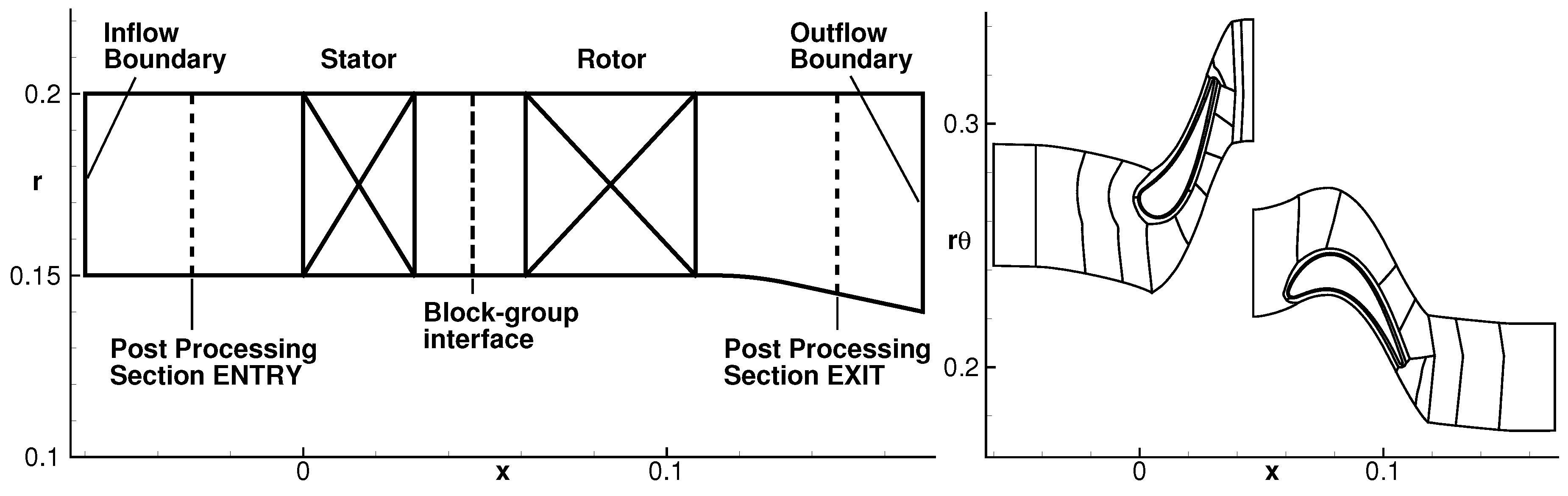
The computational domain and the structured mesh for the URANS and HB simulations are the same (see Figure 1). The mesh consists of two block groups—one for each blade row. The governing equations are solved in the relative frame of reference. Upstream and downstream of the stage, the domain is prolonged with clean duct sections of about two stator axial chord lengths. In the circumferential direction, the computational domain is reduced to one passage for each blade row.

The spatial resolution of the acoustic waves was fixed based on the acoustic axial wavelength calculated assuming a constant axial mean flow. Relevant pressure waves are resolved with at least 76 PPW (points per wavelength) and 38 PPW for the fundamental BPF and its first harmonic. According to Schnell [34], the artificial damping should be less than 0.5 dB per wavelength.

At the inflow boundary, axial uniform flow is imposed with a total pressure of 220 kPa, a total temperature of 330 K, a turbulence intensity of 5%, and a turbulence length scale of 1 $\times {10}^{-4}$ m. At the outflow boundary, the static pressure is set to 100 kPa at midspan. Those values intend to match the experiment.

The URANS simulation is resolved with 500 time steps per blade passage and 20 sub-iterations per time step. The HB calculations account for four harmonics.

3.2. Mesh Density Study

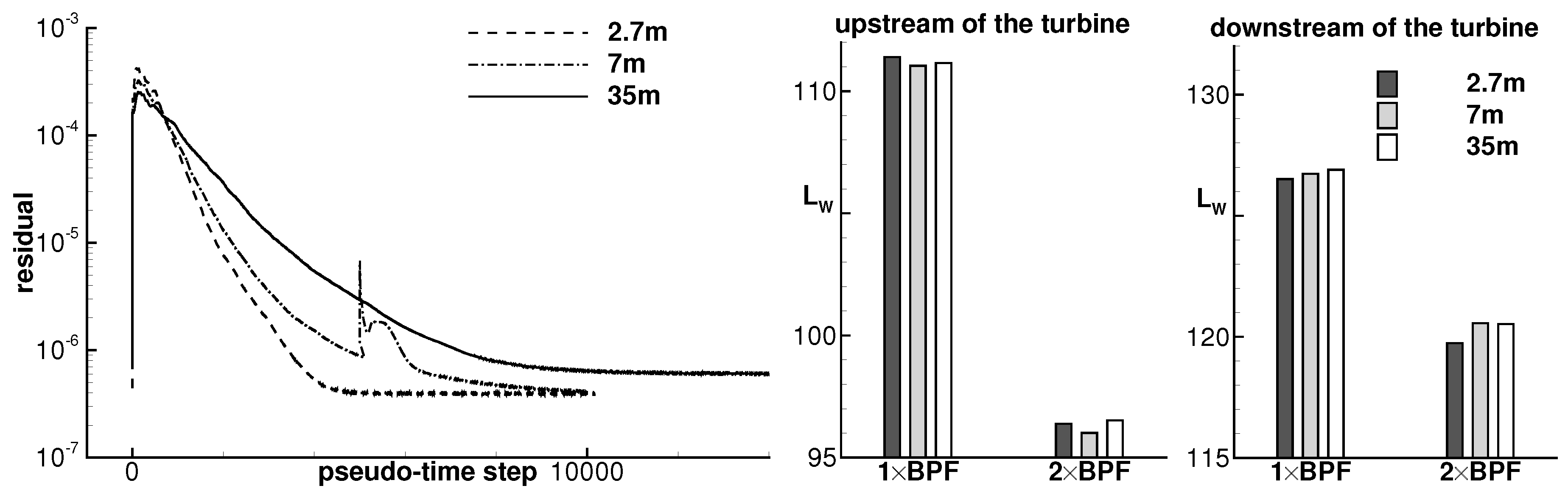
Using the HB method, a convergence study was conducted based on three block-structured meshes having a different mesh density: a coarse mesh with $2.7\times {10}^6$ cells, a medium-size mesh with $7\times {10}^6$ cells, and a fine mesh with $35\times {10}^6$ cells. Figure 2 (left) shows the $l^2$-norm of the density residual for the three meshes. All three simulations are very well converged. As expected, the larger meshes require more pseudo-time steps. The peak in the residual distribution for the medium-size mesh is due to a restart of the calculation.

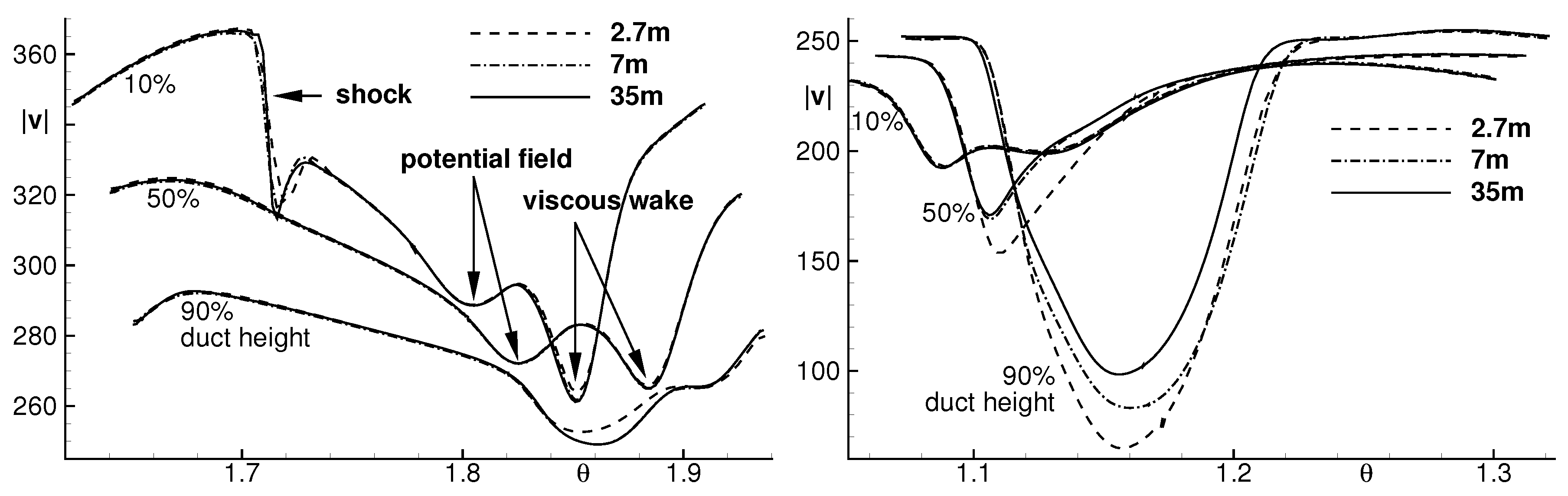
Globally, there is a very good agreement in the aerodynamic and acoustic results between the medium-size and the fine meshes. Figure 3 shows the time-averaged velocity in the stator wake and rotor wake. Downstream of the stator, the velocity jump due to a shock in the stator hub region visible at 10% duct height appears slightly steeper with mesh refinement. At mid span, the velocity distributions are identical for the three meshes. For the coarse mesh there is a small discrepancy in the stator velocity wake close to the outer duct wall at 90% duct height. Downstream of the rotor, the time-averaged flow solutions obtained with the three meshes also indicate a certain grid independency, except in the tip region at 90% span where the tip clearance vortex is strong. There the velocity deficit decreases by about 10% from the coarse to the medium mesh and again from the medium to the fine mesh. The width of the viscous wake measured at 50% depth also differs between the three meshes by about 10%.

The tip vortex is considered not to have an important impact on the generation of tonal noise in this single-stage turbine. Figure 2 (right) shows the sound power $L_W$ measured upstream and downstream of the turbine ($L_W=10{log}_{10}\left(P/P_{ref}\right)$ with $P_{ref}={10}^{-12}$ W). The discrepancy is less than 1 dB between the three meshes and maximum 0.5 dB between the medium-size and the finest one.

It was considered for the following that the medium-size mesh is suitable to simulate the flow phenomena relevant for the generation of interaction tones. This mesh is composed of about $4\times {10}^6$ cells in the stator block group and about $3\times {10}^6$ cells in the rotor block group. The larger number of cells in the stator block group is partly explained by the fact that the stator passage is broader in azimuth. Furthermore, a slightly smaller cell size was chosen in the stator domain to properly resolve the shock in the hub region.

3.3. Robustness of the XTPP Method

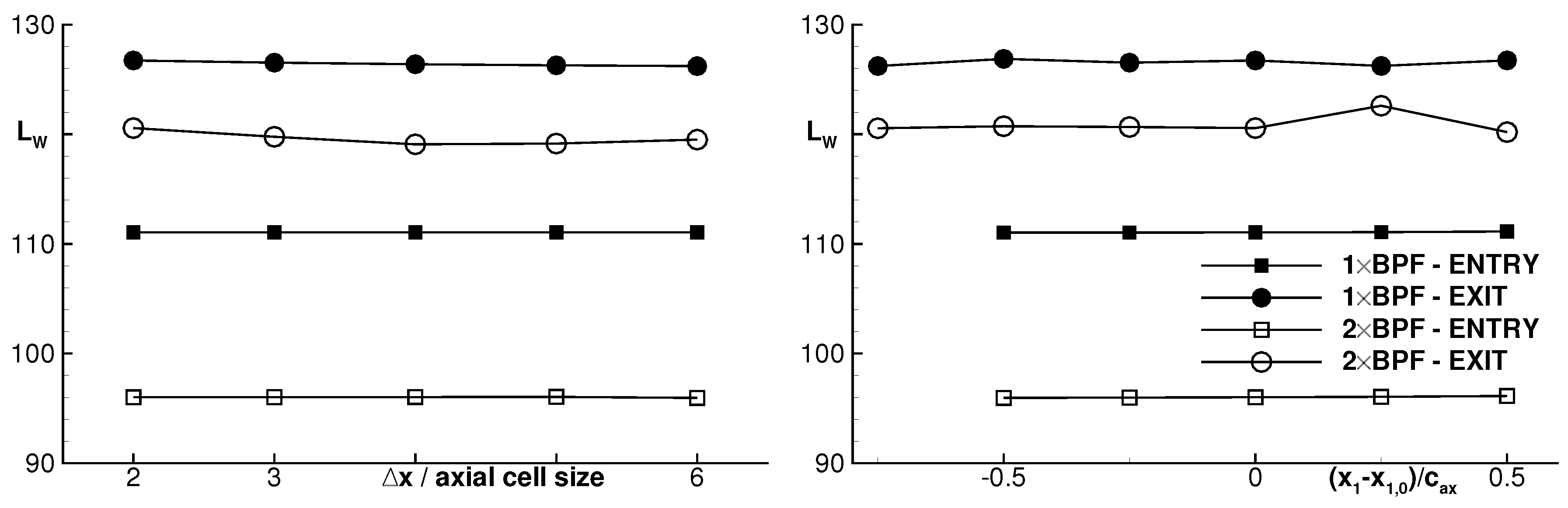
The flow solutions obtained with the HB and URANS methods are compared on an acoustic basis. The robustness of the method to calculate the tonal sound power is now evaluated. The XTPP method uses three analysis planes at which the complex pressure Fourier coefficients extracted from the unsteady flow solution are matched to a basis of eigenmodes determined analytically. Each analysis plane is a cross-sectional cut at constant axial position. In a first study, the axial spacing between the planes is varied from $\mathsf{\Delta }x=1.7$ to 5.1 mm, which corresponds approximately to the axial distance between two and six cells, respectively. The position of the first plane $x_1$, which together with $\mathsf{\Delta }x$ defines the position of all three planes, is kept constant during the variation of $\mathsf{\Delta }x$. For the analysis upstream of the turbine, we have $x_1=-0.0306$ m, which is one stator axial chord length $c_{ax}$ upstream of the stator; for the analysis downstream of the turbine, $x_1=0.14695$ m, which is about $1.28c_{ax}$ downstream of the rotor. In a second study, the axial spacing between the planes is kept constant to $\mathsf{\Delta }x=1.7$ mm and the three planes are moved in both directions upstream and downstream with a $1/4c_{ax}$ step covering a range of at least one axial chord.

The results applied to the HB solution are shown in Figure 4. The sound powers of all waves propagating away from the turbine are summed up for each frequency. Reflections back towards the turbine are significantly smaller and are not shown for the sake of clarity. In the inlet, the analysis method is very robust: the variations in sound power levels are less than 0.2 dB. In the exit section of the turbine, the variations are larger but still satisfactory: smaller than 1 dB for 1×BPF and 2 dB for 2×BPF. The higher discrepancies measured on the downstream side of the turbine have two main reasons: firstly, the mean flow strongly differs from the uniform-flow assumption applied to determine the eigenmodes; secondly, the variation in the duct geometry and as a consequence in the mean flow are in conflict with the slowly varying duct assumption, which does not allow any mode to become cut-on in the analysis section. According to this study for 2×BPF, the mode (−16,3) changes from cut-off to cut-on at some position between $(x_1-x_{1,0})/c_{ax}=0.25$ and 0.5. This strongly affects the level of the mode (−16,2). At the analysis position $(x_1-x_{1,0})/c_{ax}=0.25$, that mode is higher by about 10 dB and thereby the sum over all modes is increased by about 2 dB compared to the rest.

From now on, all acoustic results presented are obtained with the axial spacing $\mathsf{\Delta }x=1.7$ mm and the positions $x_1=-0.0306$ m and $x_1=0.14695$ m, respectively, in the inlet and the exit.

3.4. Aerodynamic and Acoustic Results: Comparison of HB and URANS

The following section aims at showing that the HB method provides similar results to the URANS method. The global performance of the stage is almost identical in both simulations, as indicated by

Table 1. Global aerodynamic performance.

	HB	URANS ${}^{\mathit{a}}$
Mass flow rate (kg/s)	6.432	6.432
Total pressure ratio (-)	2.098	2.099
Isentropic efficiency (-)	0.891	0.893

${}^a$ Determined after 25,000 time steps. HB: harmonic balance; URANS: unsteady Reynolds-averaged Navier–Stokes.

. While there are still small variations in the URANS flow solution after 25,000 time steps (50 periods) (e.g., for the mass flow rate of about 0.1%), the HB results are fully converged.

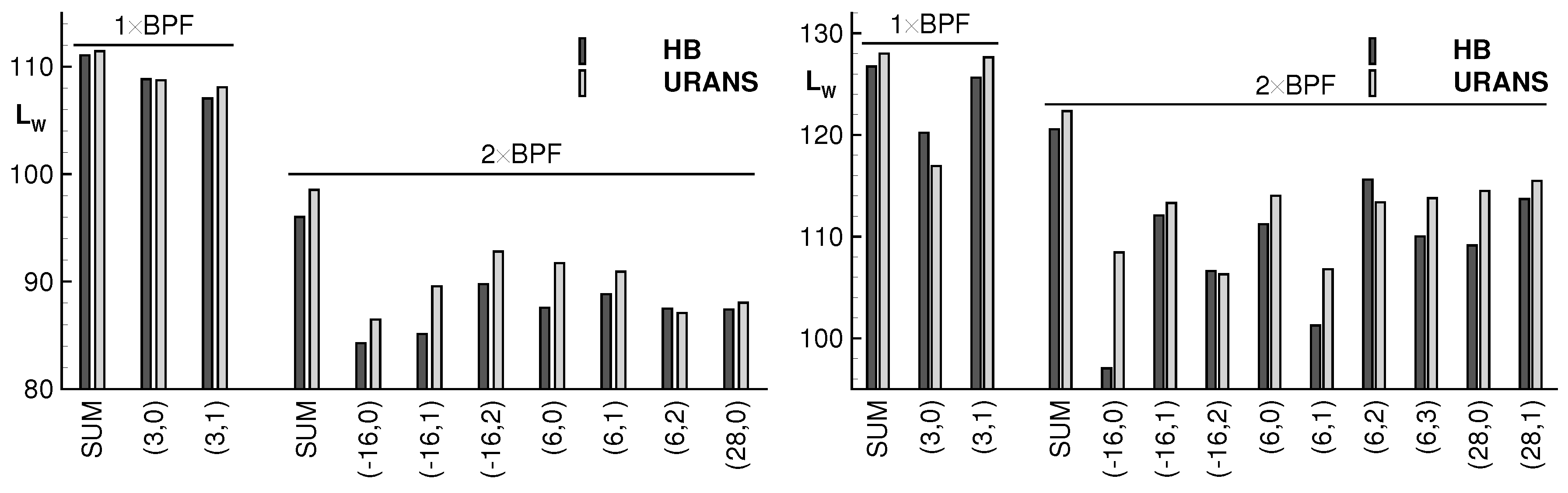
The acoustic results are summarised in Figure 5, where the sound power level is represented in total and per mode for each frequency. The azimuthal mode orders excited by the turbine at the k-th harmonic of the blade passing frequency are given by $m=kB+k^{\prime }V$ [38]. The total sound power found in each frequency tends to be smaller in the HB calculation than in the URANS calculation. Upstream of the turbine, it is smaller by about 0.4 dB and 2.5 dB and downstream by about 1.3 dB and 1.8 dB, respectively, for the fundamental BPF and its first harmonic. For individual modes, the discrepancy can be significantly larger, reaching up to 10 dB.

Those discrepancies are partly related to the different numerical methods. For instance, the number of harmonics being accounted for in the HB method is usually restricted. In this paper, only four harmonics are considered in the HB calculations. Another explanation is the convergence of the phase-lag method. This method works much better in combination with the HB method, because it is formulated in the frequency domain. A convergence study based on the modal sound power spectra obtained with the XTPP method has shown that for the HB calculation the variation for every individual mode is below $0.1$ dB after 5000 and 10,000 iterations. The convergence for the URANS calculation is less good. After 20,000 and 25,000 time steps, the sound power summed up per frequency still varies by about 0.1 dB for 1 × BPF and by about 0.6 dB for 2 × BPF. For the individual modes, the differences are significantly larger: below $1.2$ dB at 1 × BPF and up to 10 dB at 2 × BPF. A third reason for the differences between the two calculations might be due to the non-reflecting boundary conditions. They also perform better in the HB calculation.

Table 2. Difference between the sound power emitted by the turbine and reflected at the domain boundaries (dB).

	HB		URANS
	Inflow Boundary	Outflow Boundary	Inflow Boundary	Outflow Boundary
BPF	−15.8	−15.3	−11.0	−7.9
2 × BPF	−12.9	−16.8	−10.8	−4.5

shows the difference between waves propagating toward the boundaries and those backward reflected. The reflections are much stronger in the URANS calculation, especially downstream of the turbine.

4. Impact of Steady Hot Streaks

In this section, results are presented for time-periodic unsteady flow simulations in the turbine with steady hot streaks prescribed at the inflow boundary. The simulations aim at mimicking 11 equidistant and identical streaks from a hypothetical combustor ring. The same mesh as described in the first part of this paper is used, but the stator block group is duplicated in the circumferential direction. Thus, the computational domain now involves two stator passages with one imposed streak and still one rotor passage in the second block group. In total, this mesh counts about $11\times {10}^6$ cells.

4.1. Inflow Boundary Condition with Streaks

In the configuration with hot streaks, the inflow is no more uniform at the entry. At regular intervals in the azimuthal direction, 11 steady hot spots are prescribed. Those develop as hot streaks inside the domain.

The streaks disturb the static temperature T, while the static pressure p and the velocity $\mathit{v}=(v_x,0,0)$ remain unchanged. In other words, entropy is coupled into the domain but no vorticity is applied. The streaks are prescribed in terms of total pressure and total temperature. It can be shown that the temperature jump is the same for the static and the total values. The spatial distribution of the disturbance is circular and weighted with the square of a cosine function. The static temperature for the streaks is constructed with

$$T\left(d\right)\equiv T_0+\mathsf{\Delta }T{cos}^2\left(\pi d/D\right)ifd<D,$$

(1)

with $T_0$ being the background temperature, $\mathsf{\Delta }T$ the temperature disturbance amplitude, D the streak diameter, and $d={[{(y-r_{S}cos{\theta }_S)}^2+{(z-r_{S}cos{\theta }_S)}^2]}^{1/2}$ the distance to the streak centre $(r_S,{\theta }_S)$. The background flow quantities are taken from the flow solution of the configuration without streaks ($T_0\approx 328.7$ K, $v_x\approx 50.9$ m/s, and $p\approx 217,009$ Pa).

4.2. Impact of Hot Streaks on the Results

In a first simulation, the streak is set with a temperature amplitude of $\mathsf{\Delta }T=100$ K and a diameter $D=0.03$ m, which corresponds to 60% of the duct height. The radial position of the streak centres $r_S=0.175$ m is at midspan, and the circumferential position ${\theta }_S$ has been chosen so that the streak is convected approximately in the middle of two stator blades in the free passage. 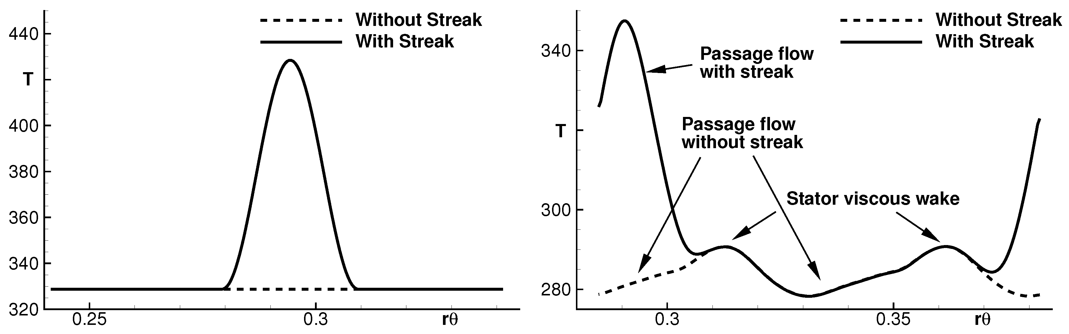Figure 6 shows the distribution of static temperature in the steady flow solution at the inflow and outflow of the stator, approximately at the streak centre radial position. The initial temperature difference of $\mathsf{\Delta }T=100$ K clearly reduces as the flow passes through the stator down to about 67 K at the stator–rotor interface. Furthermore, a bending of the hot streaks from an initial position at 50% of the span towards the hub at about 41% downstream of the stator is also observed. Those two effects were found by Papadogiannis [39] in a large-eddy simulation of a hot streak in an industrial high-pressure turbine stage. 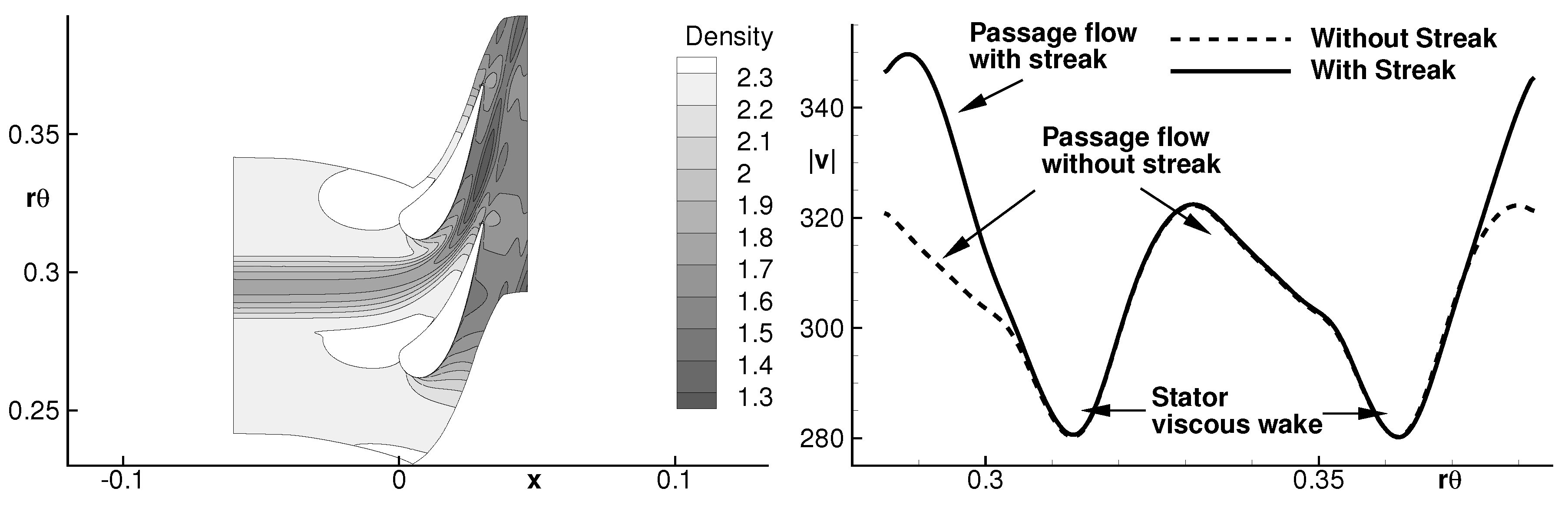Figure 7 (left) shows the density in the steady flow solution in the stator block group. The low density area upstream of the stator represents the streak. The streak contours remain almost constant during the convection toward the stator leading edge. In the stator passage, the flow is accelerated. Figure 7 (right) represents the velocity amplitude downstream of the stator with and without streaks. While the streak is imposed without velocity difference at the entry, its velocity field is significantly modified at the stator exit by the presence of the streaks. Therefore, the rotor now interacts not only with a non-uniform temperature field, but also with a modified velocity field.

The circumferential period of the incoming flow is now 11 rather than 22 without streak. This change in the periodicity of the stator wake leads to the generation of additional interaction modes whose azimuthal orders at the k-th harmonic of the blade passing frequency are given by:

$$m=kB+k^{\prime }V+k^{″}S.$$

(2)

The excitation of additional modes due to streak–rotor interaction is also reported by Mu et al. [9]. Note that the configuration without streak was simulated using the same mesh with two stator passages and the same 2D inflow boundary condition but with $\mathsf{\Delta }T=0$ K. This allows the evaluation of a signal-to-noise ratio for the additional acoustic modes due to the presence of the streaks. The operating point for the simulation with streaks has slightly changed because of the inflow boundary condition. Compared to the simulation without streak, the mass flow rate has dropped by about 0.5% whilst the total pressure ratio remains constant at 2.098.

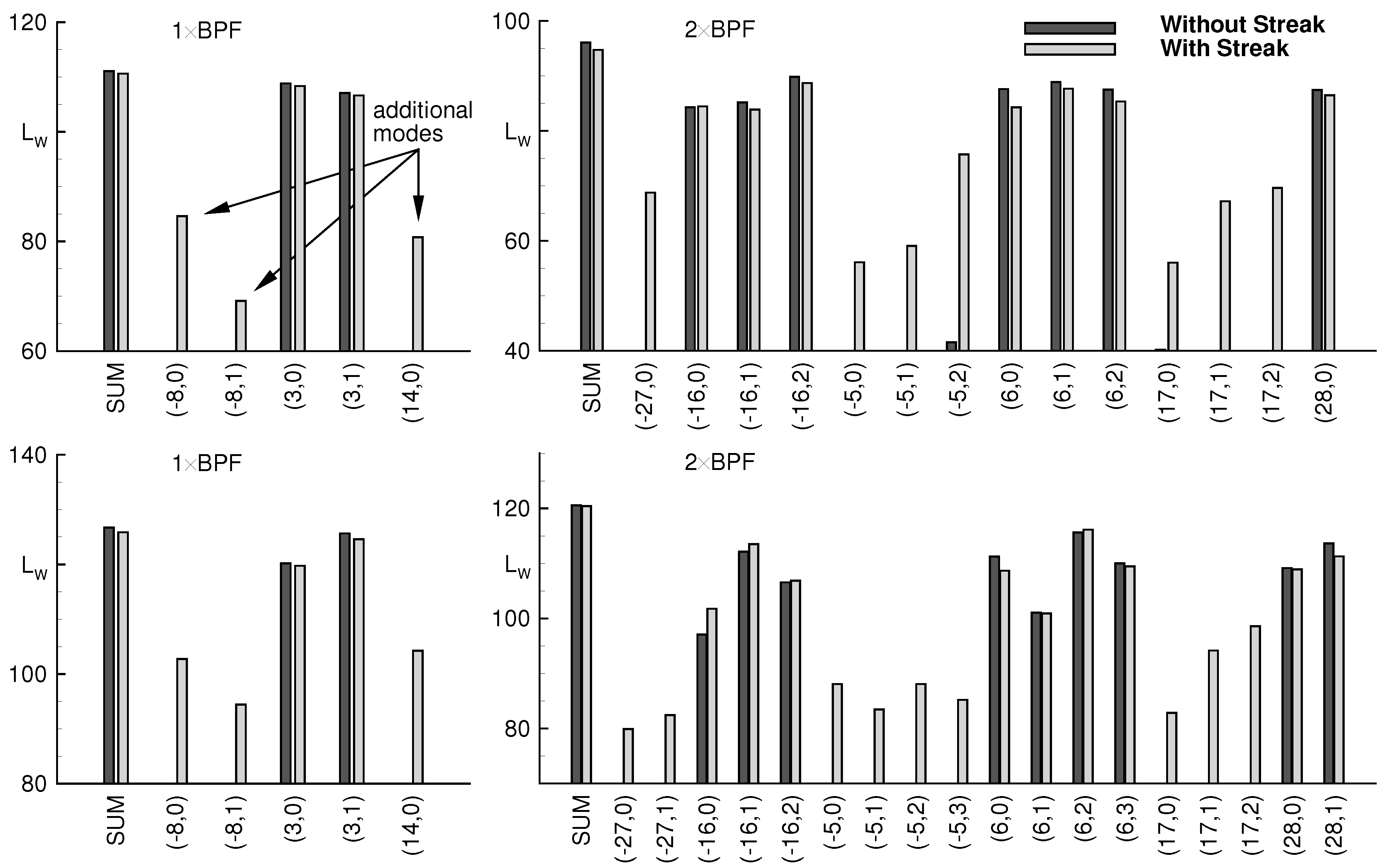
Figure 8 shows the modal sound power spectra for 1 × BPF and 2 × BPF and the total sound power level per frequency for the modes propagating away from the turbine. Clearly there are additional mode orders present in the acoustic field as a consequence of the streaks. The mode orders satisfy Equation (2): at 1 × BPF the new modes are at $m=-8$ and 14, and at 2 × BPF $m=-27$, $-5$, and 17. Those additional acoustic modes transport significantly less power (≈−20 dB) than the modes whose azimuthal orders correspond to the original stator–rotor interaction.

Table 3. Acoustic sound power level (dB) propagating away from the turbine with and without streaks.

	Upstream		Downstream
	Without Streak	With Streak	Without Streak	With Streak
1 × BPF additional modes	(55.8 ${}^a$)	86.2	(76.1 ${}^a$)	106.8
1 × BPF original modes	111.1	110.6	126.7	125.8
2 × BPF additional modes	(46.3 ${}^a$)	77.8	(68.8 ${}^a$)	100.8
2 × BPF original modes	96.0	94.6	120.6	120.4

${}^a$ These values denote numerical noise.

gives the sound power of the additional and original modes. For the simulation without streaks, the acoustic sound power found in the additional modes is due to numerical noise in the simulation. The signal-to-noise ratio given by the simulation without streaks is about 50 dB, which provides confidence that the relatively small sound power found in the additional modes in the simulation with streak is physical. The comparison between both simulations also shows a minimal decrease of the sound power due to the streaks for the modes corresponding to the original stator–rotor interaction, which is also apparent in the integrated sound power level. This reduction is about 0.5 dB and 1.3 dB upstream of the turbine and about 0.8 dB and 0.2 dB downstream. It might be worth mentioning that this reduction is noticeable for most but not all individual modes. For instance, downstream of the turbine the amplitude of the mode $m=-16$ increases with the streaks (see Figure 8 bottom right).

4.3. Variation of the Streak Temperature Amplitude and the Streak Diameter

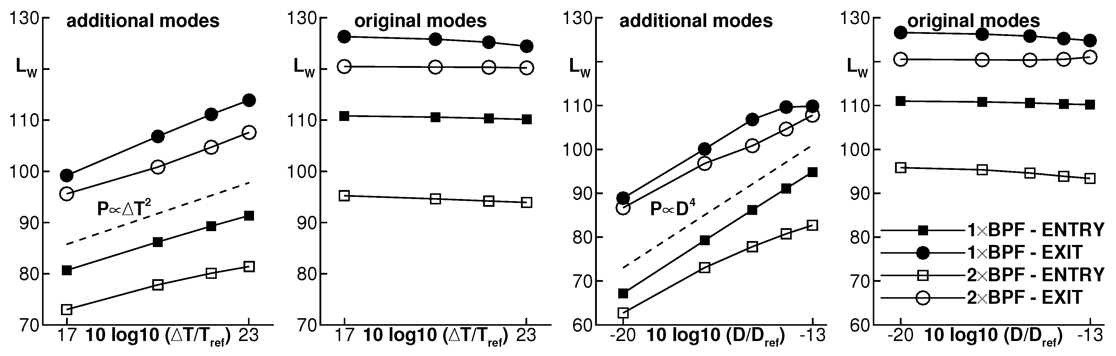
In the following, two parameter variations are presented. In the first study, the streak temperature is varied from $\mathsf{\Delta }T=0$ to 200 K in 50 K steps while the streak diameter remains unchanged ($D=0.03$ m). In the second study, the streak diameter is varied from $D=0$ to 0.05 m (100% duct height) in 0.01 m steps with a constant temperature amplitude $\mathsf{\Delta }T=100$ K. Figure 9 shows among others the sound power level of the additional modes coming from the streaks. The amplitude evolution seems to follow a simple scaling law of the type:

$$P\propto {\mathsf{\Delta }T}^{\alpha }{D}^{\beta }.$$

(3)

The exponents $\alpha$ and $\beta$ determined by linear regression and the corresponding coefficients of determination $R^2$ are given in

Table 4. Exponents $\alpha$ and $\beta$ and coefficients of determination $R^2$ for modelling the integrated sound power of the additional modes due to the streaks.

	Upstream		Downstream		Upstream		Downstream
	$\mathit{\alpha }$	${\mathit{R}}^{\mathbf{2}}$	$\mathit{\alpha }$	${\mathit{R}}^{\mathbf{2}}$	$\mathit{\beta }$	${\mathit{R}}^{\mathbf{2}}$	$\mathit{\beta }$	${\mathit{R}}^{\mathbf{2}}$
1 × BPF	1.78	1.000	2.45	0.999	3.96	1.000	3.16	0.968
2 × BPF	1.41	0.993	1.98	0.995	2.88	0.990	2.96	0.996

. The exponent indicating the temperature dependency varies within the range $1.4\le \alpha \le 2.5$, and that for the diameter verifies $2.9\le \beta \le 4.0$.

The original modes remain dominant in all simulations. Their sound power levels change very little. With the maximal temperature amplitude or the maximal streak diameter, the integrated sound power from the original modes reduces by about 1 dB for each frequency on the upstream side of the turbine. On the downstream side, it reduces by 1.5 to 2 dB at 1 × BPF and increases by 0 to 1 dB at 2 × BPF.

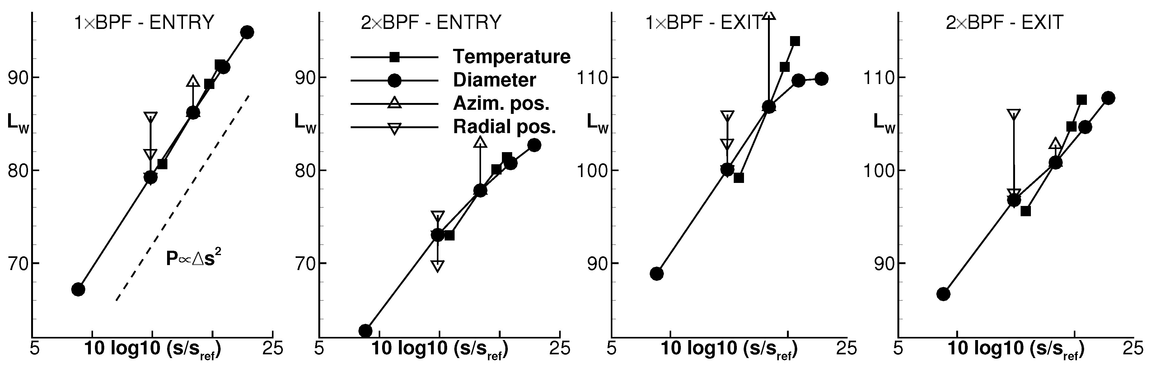
The same values of sound power are shown again in Figure 10 as a function of the entropy flow due to the streak. For each simulation, the entropy flow through the entire inflow boundary is determined using the following formula:

$$s=\int \rho v_x{c}_{v}log\frac{p/p_0}{{(\rho /{\rho }_0)}^{\mathsf{\gamma }}}dA.$$

(4)

With the reference values $p_0$ and ${\rho }_0$ consistently chosen for all simulations, the increase of the entropy flow due to the streak $\mathsf{\Delta }s$ can be determined by the difference of the entropy flow for the simulations with and without streaks. The sound power can be modelled with

$$P\propto {\mathsf{\Delta }s}^{ϵ}.$$

(5)

Detailed values of $ϵ$ are given in

Table 5. Exponent $ϵ$ and coefficients of determination $R^2$ for modelling the summed up sound power of the additional modes due to streaks.

	Variation of the Temperature				Variation of the Diameter
	Upstream		Downstream		Upstream		Downstream
	$\mathit{ϵ}$	${\mathit{R}}^{\mathbf{2}}$	$\mathit{ϵ}$	${\mathit{R}}^{\mathbf{2}}$	$\mathit{ϵ}$	${\mathit{R}}^{\mathbf{2}}$	$\mathit{ϵ}$	${\mathit{R}}^{\mathbf{2}}$
1 × BPF	2.24	1.000	3.08	1.000	1.97	1.000	1.57	0.967
2 × BPF	1.78	0.998	2.48	0.988	1.43	0.989	1.47	0.996

together with the coefficients of determination. With $ϵ$ being in the range from 1.4 to 3.1, these results are similar to what is proposed by Marble and Candel [3]. In that one-dimensional theory on sound waves generated by the convection of entropy spots through a sub-sonic nozzle, the sound pressure amplitude is directly proportional to the entropy fluctuation, and thus the sound power is proportional to the entropy fluctuation squared. This similarity between theory and the numerical results regarding the relationship between entropy disturbance and sound power might indicate that the additional acoustic modes could be due to entropy noise. However, there is no certainty for this source mechanism being dominant concerning the additional modes in the presented simulations, because the streaks during their convection through the stator also modify the velocity field as shown before in Figure 7. The force-induced sound sources on the rotor surface resulting from the interaction of the velocity field with the rotor could be important and dominant, too.

In addition to the variation of the streak temperature amplitude and the streak diameter, Figure 10 also shows results for a variation of the streak radial and azimuthal position. The radial position was also investigated at 20% and 80% of the duct height (using a streak diameter of $D=0.02$ m) and the azimuthal position was changed to ${\theta }_S\approx 1.85$ rad (with $D=0.03$ m). There the streak hits a stator leading edge, is divided in two and convected on both sides of the stator vane. These two parameters also appear to have a significant effect on noise. The sound power of the additional modes can increase by 5 to 10 dB due to those changes. The variation obtained by changing the streak radial position might be related to the variation of the mean flow Mach number in the rotor. Furthermore, the streaks might be moved to more or less acoustic effective positions when their radial position is changed. The streak azimuthal position defines whether the stator passage flow is affected or the flow in the vicinity of the vane. In contrast to Figure 7, the velocity field in the passage flow downstream of the stator appears unchanged, but the velocity deficit in the stator wake is significantly reduced (by about 27% of its depth) when the streak hits the stator.

5. Conclusions

In the first part of this paper dedicated to the configuration without streaks, it was shown that the newly implemented HB method provides similar results to the URANS method which has already been validated against experimental data. In this example, the HB calculation ran 20 times faster than the URANS calculation. Furthermore, the phase-lag method and the non-reflecting inflow and outflow boundary conditions perform better in combination with the HB method, which enables a better convergence of the results. Those advantages made it possible to carry out a parameter study on the impact of steady hot streaks with a variation of the temperature amplitude, the diameter, and the radial and azimuthal positions.

Acoustic waves due to the streaks–rotor interaction are clearly evidenced upstream and downstream of the turbine. However, the sound power of the corresponding acoustic modes is significantly smaller than that radiated by the stage alone (without streaks). This was confirmed in the test campaign posterior to the numerical study.

The relationship between the sound power of the additional acoustic waves and the streak entropy difference verifies approximately $P\propto \mathsf{\Delta }{s}^2$. This result is similar to that proposed by Marble and Candel [3], which describes the noise generation due to the convection of entropy-spots through a sub-sonic nozzle.

The streaks were imposed in the form of a temperature disturbance with the static pressure and the velocity kept constant. As the streaks pass the stator, they are cooled down but also more strongly accelerated than the rest of the flow. As a consequence, the speed is slightly higher in the wake of the streaks as they reach the rotor fan face. Therefore, the rotor interacts with both a modified entropy field and a modified velocity field.

It is not known at this point whether the observed acoustic waves with additional azimuthal mode orders are due to the streak entropy being convected through the rotor, due to unsteady pressure forces on the rotor surface caused by the modified velocity field at the rotor face, or both effects.