Improved Turbulence Prediction in Turbomachinery Flows and the Effect on Three-Dimensional Boundary Layer Transition ^†

Abstract

For the numerical prediction of turbomachinery flows, a two-equation turbulence model in combination with a proper transition model to account for laminar boundary layers and their transition to turbulence is state of the art. This paper presents the ability of such a method (k-ω + γ-Re_Θ) for turbulence prediction and the effect on three-dimensional boundary layer behavior. For this purpose, both applied models (turbulence and transition) are improved to better account for turbulence length scale effects and three-dimensional transition prediction (Bode et al., 2014 and 2016), since these are the main deficiencies in predicting such kinds of flows. The improved numerical method is validated and tested on existing turbine cascades with detailed experimental data for the viscous regions and additionally on a low-speed axial compressor rig where wake-induced transition takes place.

1. Introduction

Nowadays, the industrial design of turbomachines and their components is conducted with three-dimensional (3D) Navier–Stokes solvers (computational fluid dynamics, CFD). These mostly unsteady Reynolds averaged Navier–Stokes (U)RANS solvers are able to simulate multistage 3D blade passages with unsteady flow effects. Hence these types of solvers will be the key design tool for today and tomorrow [1]. An up-to-date numerical method for turbomachinery flows and their applications is the combination of the two equation k-$\omega$ turbulence model after Wilcox (1988) [2] and the $\gamma$-Re_Θ transition model after Menter and Langtry [3] which is used to incorporate laminar boundary layers and their transition to turbulence. These effects are significant in e.g., low-pressure turbine flows and also to a smaller degree in compressors. From a present-day perspective, this numerical method is able to predict the midspan boundary layer behavior on the airfoils in an adequate way. Nevertheless, even in a simple cascade there are still uncertainties in the prediction of the two-dimensional (2D) midspan and especially of three-dimensional boundary layer behavior on the airfoils and additionally on the sidewalls (hub and tip) and their interaction with the secondary flow phenomena. In 2D flows, the turbulence quantities and their prescription at the free stream inlet will influence the boundary layer state. While considering laminar boundary layers in CFD, resulting in highly improved total pressure loss prediction compared to a fully turbulent CFD, the correct prescription of the turbulence quantities, like free stream turbulence intensity as one of the main impact factors, will in turn influence the laminar-turbulent boundary layer prediction as shown by Bode et al. [4]. Moreover, the occurrence and numerical prediction of laminar boundary layer regions on the sidewall and their effect on the downstream flow of a blade row is not completely understood, cf. [5,6]. An attempt to improve prediction accuracy in this region was made by Bode et al. [7], where the $\gamma$-Re_Θ transition model was recently extended to three-dimensional boundary layer transition after Menter and Smirnov [8] in combination with the shear stress transport (SST) model [9] and validated against general test-cases and also successfully applied to three-dimensional turbomachinery flows. This method showed good agreement with experimental data. In a 3D multistage component environment, the prediction accuracy of the downstream blade rows is highly dependent on the correct flow prediction of the upstream blade rows and their turbulent quantities. Thus, an improved numerical method is necessary for the design of new multistage turbomachines and their components. For example, an increased prediction accuracy of the turbulent kinetic energy (turbulence intensity) and its dissipation will lead to an improved boundary layer transition prediction. This, in turn, leads to a better prediction of the wake of the airfoils and hence, more accurate flow condition for the downstream blade row.

In the present paper, the k-$\omega$ turbulence model after Wilcox (1988) [2] with a modification after Bode et al. [10] to improve the turbulence prediction in combination with the transition model after Menter and Langtry [3] and its extension to three-dimensional boundary layer transition after Menter and Smirnov [8] will be used to further improve the turbulence prediction and hence, the transitional behavior and its impact on the loss prediction. Therefore, the improved numerical method will be validated against test-cases with increasing complexity and will present the ability of the used numerical method to accurately predict the turbulence and transitional behavior of three-dimensional single and multistage turbomachinery test-cases.

2. Numerical Method

The parallel CFD-solver TRACE of DLR (Cologne, Germany), as an up-to-date numerical method, has been applied, cf. Marciniak et al. [11]. The turbulence is modeled by the two-equation k-$\omega$ model of Wilcox (1988) [2], together with the Kato-Launder [12] fix for the stagnation point anomaly. The boundary layer transition has been modeled by the two-equation $\gamma$-Re_Θ model of Menter and Langtry (2009) [3]. The model evaluates the local flow features to facilitate natural, bypass, and separation-induced transition as well as relaminarization and wake-induced transition. Furthermore, the model is extended by Bode et al. [7] to incorporate cross-flow induced transition in three-dimensional boundary layers according to the model after Menter and Smirnov [8]. Herein an indicator function is proposed which gives an approximation of the cross-flow integral used by Arnal [13] in his experimentally-based cross-flow stability criterion (C1 criterion). This criterion reads as follows:

$$\frac{R{e}_{\delta ,2t}^{*}}{f\left(H_S\right)}>150,$$

(1)

where $f\left(H_S\right)$ is a function of the streamwise shape factor of the boundary layer.

$$f\left(H_S\right)=\left\{\begin{array}{cc}\frac{300}{\pi }\arctan \left(\frac{0.106}{{\left(H_S-2.3\right)}^{2.05}}\right),\hfill & 2.3<H_S<2.7\hfill \\ 150,\hfill & H_S<2.3\hfill \end{array}\right.$$

(2)

In this formulation 150 is a calibration constant corresponding to the critical Reynolds number where cross-flow transition takes place. The new cross-flow induced transition onset trigger within the $\gamma$-Re_Θ model formulation $F_{onset,CF}$ is given as follows:

$$F_{onset,CF}=\min \left(\max \left(100·\left(T_{C1,local}-1.0\right),0.0\right),1.0\right)$$

(3)

with 100 as a speed up factor for the cross-flow induced transition process [14]. The cross-flow transition trigger will now be evaluated against the two-dimensional transition trigger $F_{onset,\gamma }$ of the baseline $\gamma$-Re_Θ model

$$F_{onset,\gamma }=\max \left(F_{onset2}-F_{onset3},0\right)$$

(4)

as an additional survey like

$$F_{onset}=\max \left(F_{onset,\gamma },F_{onset,CF}\right).$$

(5)

Turbulence length scale effects on turbulence and transition prediction have been incorporated into the respective models, cf. Bode et al. [10]. The validation of today’s CFD-solvers especially against experimental cascade data with medium or high inflow turbulence intensity from 3 ≤ Tu ≤ 10% and in combination with moderate turbulence length scales (l_T∼0.01 m), (l_T/l∼0.1 with l∼0.1 m chord of a typical turbine cascade) ends up in an unphysical, too high eddy viscosity, leading to a false prediction of the turbulence and, hence, boundary layer flow due to the violation of the realizability constraint. To avoid this behavior, the CFD user often changes the turbulence length scale to fit the transitional data. In addition, the application of modified turbulence models (e.g., Durbin’s realizability constrain [15]) sometimes leads to an unphysical behavior around the leading edge and along more than 60% of the passage suction side where the eddy viscosity is damped too harshly. Therefore, the k-$\omega$ turbulence model after Wilcox (1988) is modified, so that the improved behavior regarding overall characteristics and boundary layer development is given and the unphysical behavior of the eddy viscosity is reduced. For this reason, a criterion for the determination of viscous regions (boundary layers and wakes) has been developed as an additional element of the implemented approach (cf. [10]). This criterion is based on the large values of turbulent dissipation rate $\omega$ in the vicinity of viscous walls. It takes the relationship between the turbulent dissipation rate estimated from the k-$\omega$ turbulence model and the turbulent dissipation rate in the free stream ${\omega }_{FS}$ of the flow estimated by the new approach. The effect of their very high ratio in the boundary layer and wakes is used to separate them from the free stream

$$b_v=\min \left(\max \left(\left(\frac{\omega }{{\omega }_{FS}}\right),0.1\right),1.0\right).$$

(6)

The time-scale bound is only applied in these viscous regions, effectively preventing the eddy viscosity destruction in non-viscous areas by multiplying the time-scale bound by a factor $b_v$, which is 1.0 in the boundary layer and the wake region and 0.1 in the free stream (cf. [10])

$${\mu }_T=\frac{\rho k}{\max \left(\omega ,b_{v}S\right)}.$$

(7)

In the post-processing, integral boundary layer parameters are determined by integration of the velocity field perpendicularly to the blade surface up to a point where the total pressure has increased by 99% of the whole velocity defect, cf. [16]. Throughout this paper, the boundary layers of all no-slip boundaries are highly resolved with a dimensionless wall distance of the wall adjacent cells down to $y^{+}\approx 1$ as a result of performed grid sensitivity studies for all used test-cases. Depending on the test-case, the convergence of the simulations was achieved after 2000–10,000 iterations, and was characterized by a density residual drop of at least three orders of magnitude and a relative difference of in- and outlet massflow ≤10⁻³.

3. Cascade Test-Cases

One of the main focuses of this paper lies with the incorporation of laminar-turbulent boundary layer transition in three-dimensional turbomachinery flows, especially turbine flows. In the literature there exists many investigations (numerically and experimentally) with regard to this topic. The main conclusion is that the general fully turbulent inlet boundary layer in a cascade flow (measurements by Vera et al. [17] indicate an at least transitional boundary layer at the hub of their low-pressure turbine rig) separates in front of the leading edge due to the pressure gradient in combination with the horseshoe vortex. Downstream of the separation a new boundary layer forms which is laminar based on measurements by Moore and Gregory-Smith [18] and Holley et al. [19] or large eddy simulations by Cui et al. [20]. This new laminar boundary layer is highly three-dimensional and hence, after Schlichting [21], sensitive against instabilities because of the inflection point within the boundary layer profile. Thus, it will undergo a laminar-turbulent transition process in the cross-flow direction [17]. For this purpose, the recently extended $\gamma$-Re_Θ transition model after Menter and Langtry [3] in combination with the improved turbulence prediction [10] shows its capability to better predict these kinds of flows and will now be shown as a follow up to Bode et al. [7] in more detail on the Durham and Langston cascades. Later on, the ability of the improved numerical method on multistage test-cases will be shown, too.

3.1. Durham Cascade

The Durham turbine cascade is a widely known and used CFD validation test-case. The cascade has been described in detail earlier, see for instance Walsh [22], Moore [23] and Moore and Gregory-Smith [18]. The cascade consists of six blades which have a profile typical of a high pressure turbine rotor. For a design inlet angle ${\beta }_1$ = 42.75° a turning above 110° is achieved. With an axial blade chord l_ax = 181 mm and an outlet Mach number Ma₂ = 0.1 a a Reynolds number, based on axial chord and exit velocity, Re= 4.0 × 10⁵ is obtained. The turbulence intensity and turbulence length scale are measured after Moore et al. [18] as Tu₁ = 5.6% and l_T = 9.4 mm (l_T/l∼0.04) and prescribed at the inlet of the computational domain. Contrary to the design an inlet angle ${\beta }_{\mathrm{IN}}$ = 43.5° was measured in the experiments and also prescribed as boundary condition. For more details about the numerical setup and first results on the use of the extended $\gamma$-Re_Θ transition model, see Bode et al. [7].

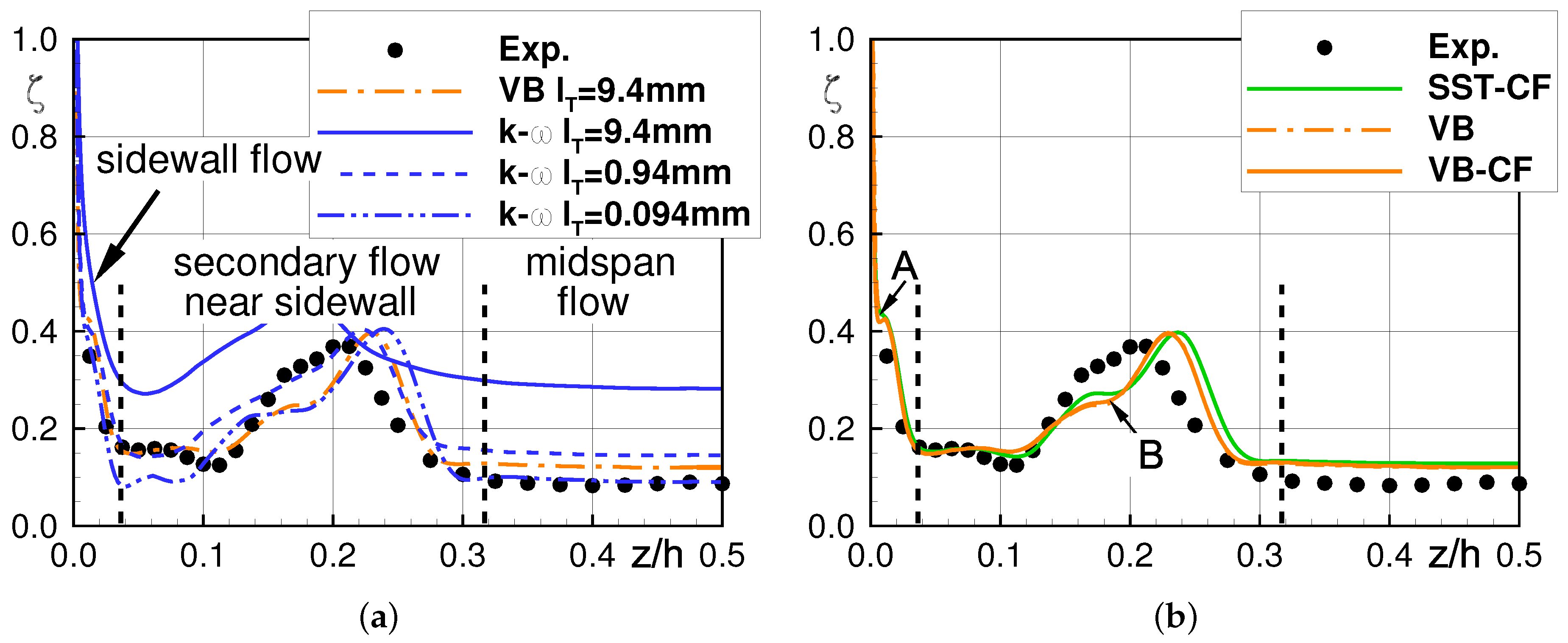
3.1.1. Spanwise Distribution

For evaluation purposes, numerical results of the pitchwise averaged spanwise distribution ($z/h$) of the total pressure loss coefficient are shown and compared against experimental results [23] in Figure 1.

Besides the numerical results of the present investigated k-$\omega$ Wilcox (1988) turbulence model with the extension after Bode et al. [10] to incorporate turbulence length scale effects in combination the $\gamma$-Re_Θ transition model after Menter and Langtry (hereafter named VB), additional results of the k-$\omega$ turbulence model after Wilcox (1988) without the extension after [10] in combination with the $\gamma$-Re_Θ transition model are shown (k-$\omega$, l_T = 9.4 mm) and different integral length scales as inlet boundary conditions are applied to emphasize the improved turbulence prediction and the effect not only on the two-dimensional midspan but also on the three-dimensional flow near the sidewalls, cf. Figure 1a.

The outlet of the cascade is here divided in three parts: (i) the midspan flow region ($0.32\le z/h\le 0.50$) where 2D flow is to be assumed, (ii) the secondary flow region near the sidewall ($0.04\le z/h\le 0.32$) where the the secondary flow phenomena like horseshoe and passage vortex are interacting with the suction side boundary layer and (iii) the sidewall flow region ($0.00\le z/h\le 0.04$) where mostly the newly formed laminar sidewall boundary layer will have an effect on the total pressure loss production.

Starting with the midspan region, the typical behavior of varying prescribed turbulence length scales is seen. A value of l_T which corresponds to the experimental hotwire measurements [18] results in a higher total pressure loss prediction due to a fully turbulent suction side boundary layer because of the unphysical production of turbulent kinetic energy at the leading edge, cf. [10]. With lower prescribed l_T values compared to the experimental ones the prediction comes closer to the experimental data. Only the improved turbulence model (VB) is able to correctly predict the total pressure loss at midspan with an l_T from the experiments.

The region where the secondary flow dominates a comparable behavior is seen. The numerical result for k-$\omega$ l_T = 9.4 mm gives a false prediction of the trend and the level of the total pressure loss due to the overproduction of turbulent kinetic energy, cf. [10]. A somewhat smaller value gives an adequate result where the smallest l_T value again results in a too small prediction of $\zeta$. The numerical results for VB are again in best agreement with the experimental data.

The sidewall flow seems to be insensitive to the turbulence length scale except for the highest l_T. The effect of the extension to three-dimensional boundary layer transition with the extended $\gamma$-Re_Θ transition model (VB-CF) is shown in Figure 1b. Here, additional results for the extended transition model with the SST model after Menter [9] are given (SST-CF). The first conclusion is that both turbulence models with the extended transition model will give almost the same good result. The VB and VB-CF predict the midspan flow and the secondary flow region slightly better than SST-CF. Moreover, the effect of the cross-flow extension here is negligible. The areas A and B show an effect of the locally occurring three-dimensional predictions due to the extended transition model compared to the original formulation. This can be seen in the following.

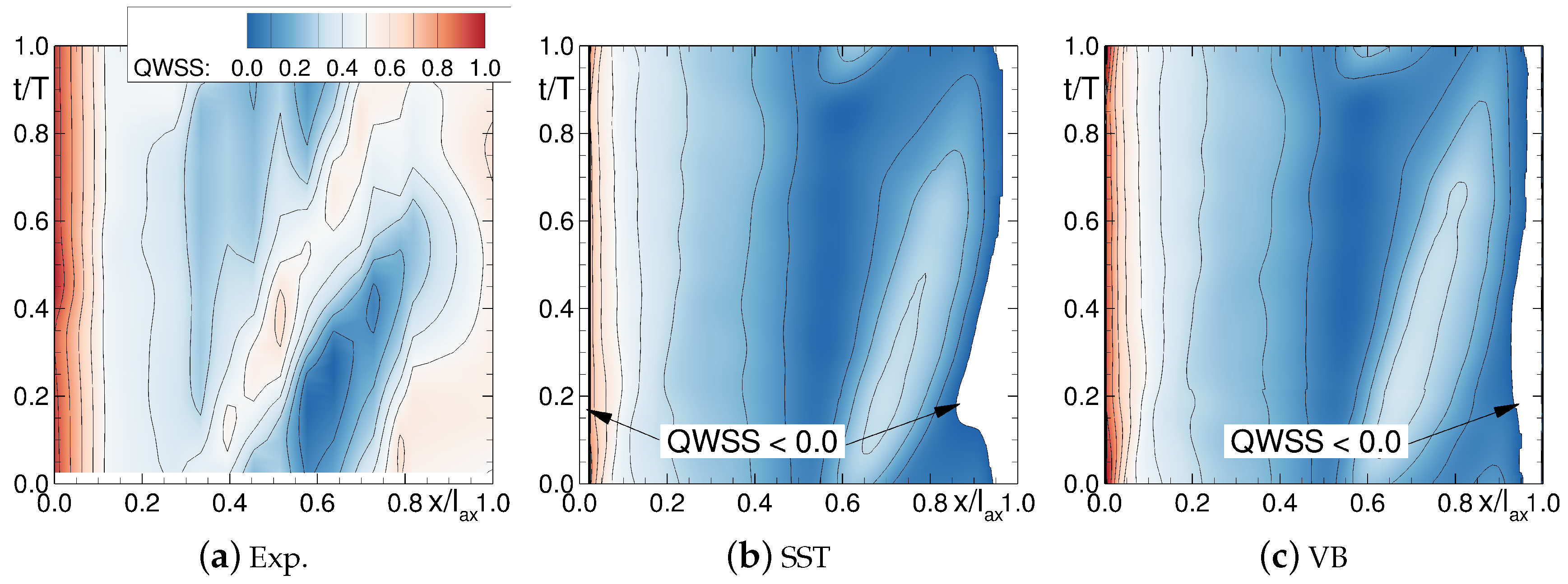
3.1.2. Boundary Layer Behavior

In Figure 2a,b differences between numerical results for predicted ${\gamma }_{eff}$ with VB-CF and VB are plotted to show the effect of the cross-flow extension to the transition model on the boundary layer behavior on the sidewall and suction surface. The extended transition model leads to a stronger prediction of the suction-side ② and pressure-side ① leg of the horseshoe vortex and hence, in combination to a stronger impingement on the suction side at ③. In addition to that, the separation line of the formed passage vortex on the sidewall ④ is also more strongly predicted. The impingement on the suction side ③ is also seen on the suction side plot in Figure 2b where the numerically predicted intermittency is also more pronounced. This is also true for the separation or lift-off line of the horseshoe vortex of the suction surface ⑤. Some minor differences on the suction surface may be identified near the laminar turbulent transition zone ⑥.

Finally, the cross-flow extension of the $\gamma$-Re_Θ transition model only shows local improvements to the prediction of the secondary flow phenomena but does not change the overall results, like shown for the total pressure loss, in this case. Since the original formulation of the transition model captures the basic behavior of the secondary flow, there is no benefit in switching on the turbulence model in these regions. In summary, the cross-flow extension leads to a locally more pronounced identification of three-dimensional secondary and boundary layer behavior but does not affect the overall flow in either a positive or a negative way.

When continuing with the improved turbulence prediction, Figure 1b indicates a closer agreement between VB and the experimental data as compared to the SST method. This is due to the better prediction of the turbulent secondary flow in the case of VB where the pressure-side leg of the horseshoe vortex and later on the passage vortex, whose are the main dominators of the secondary flow, are better predicted. This will be shown by means of the next test-case.

3.2. Langston Cascade

Besides the Durham cascade, the Langston cascade is a famous cascade test-case in the open literature and is also used by researchers such as Langston et al. [24], cf. Graziani et al. [25] and Holley et al. [19]. Like the Durham cascade, the Langston cascade is also used to determine the state of the newly formed boundary layer on the sidewall of the cascade. Likewise to the Durham cascade, the Langston cascade provides detailed experimental data on the suction and sidewall surfaces to determine the boundary layer state which indicates the trajectory of the formation of the secondary flow features. Surface static pressure and skin friction coefficients on suction side and sidewall in combination with limiting streamlines provide a solid validation basis for the applied numerical method. As already mentioned, for a correct prediction of the total pressure outlet, the accurate prediction of the secondary flow and its interaction (trajectory) with the viscous regions like suction side boundary layer are necessary. Figure 3 shows experimental and numerical results for the static pressure coefficient distribution for varying spanwise slices on the Langston cascade.

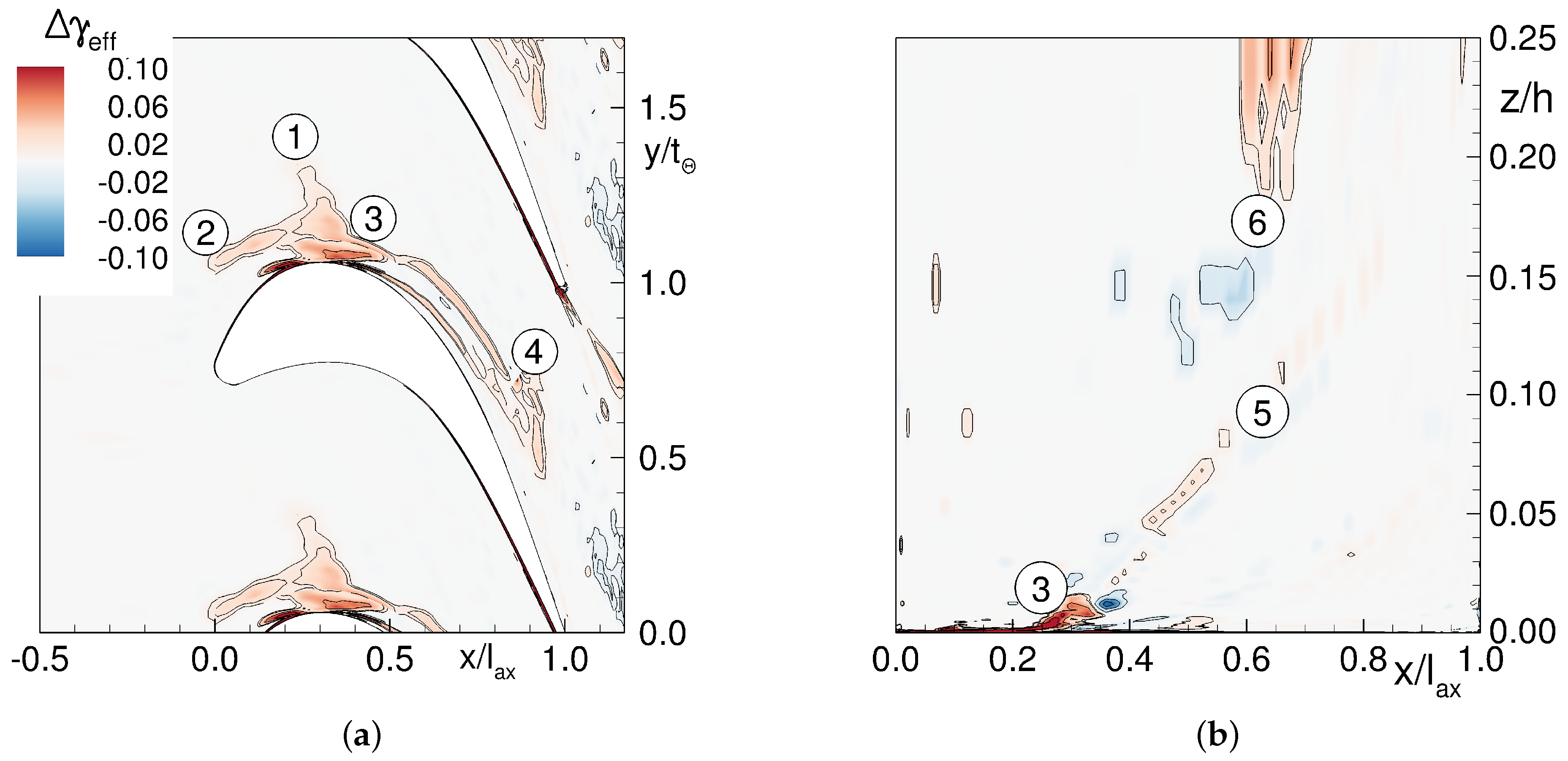
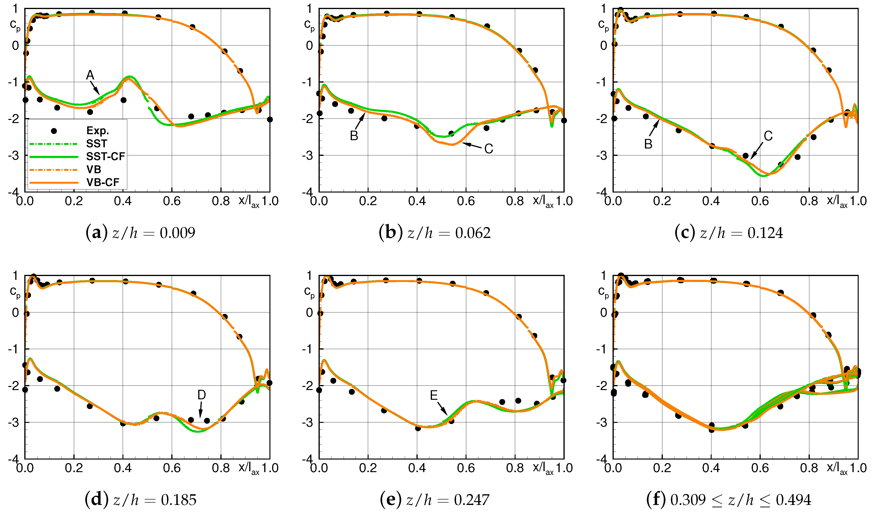
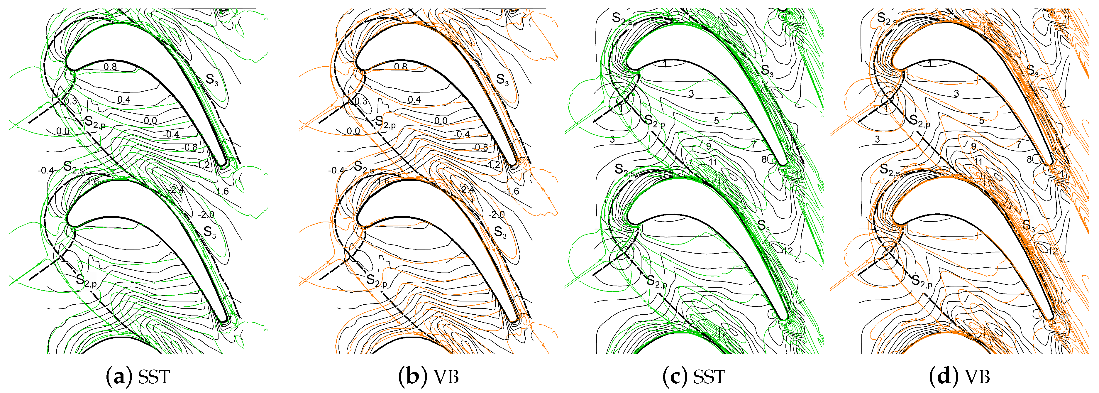
3.2.1. Suction Side Flow

Additionally to the former investigations, both model combinations (VB and SST together with the original $\gamma$-Re_Θ) are also extended with the cross-flow extension (VB-CF and SST-CF) indicating just small (below 1%) local differences (Figure 3a region A). Starting at midspan in Figure 3f, all combinations show a good prediction compared to experimental data. This holds for the next spanwise position in Figure 3e where the VB model gives perhaps a paper-thin better result than the SST (Figure 3e region E). This is more pronounced in regions D and C (in Figure 3c,d, respectively) coming closer to the sidewall where the interaction between the secondary flow and the suction side is stronger in Figure 3c,d. Closest to the wall at $z/h=0.062$ and 0.009 the favorable prediction with the VB is still present except for region C in Figure 3b.

3.2.2. Sidewall Flow

This better prediction of the static pressure coefficient distribution on the blade of the Langston cascade can be traced back to the origin of the secondary flow on the sidewall of the cascade. In Figure 4 experimental and numerical results for static pressure Figure 4a,b as well as skin friction coefficient distribution in Figure 4c,d on the sidewall of the Langston cascade are shown. Since the cross-flow extension to the transition model has in this study only local effects on the numerical prediction as seen above, just numerical results with the original $\gamma$-Re_Θ transition model in combination with VB and SST turbulence model are given. In the experimental results (black lines) in Figure 4 it can be seen that the inlet boundary layer on the sidewall separates at the horseshoe vortex lift-off lines (S_2s and S_2p), wraps around the leading edge of the cascade and forms the secondary flow downstream.

The characteristic points in the c_p and c_f plots are now the stagnation point in front of the leading edge, where the inlet sidewall boundary layer separates and will be divided and the interaction of the pressure-side leg of the horseshoe vortex with the new formed boundary layer on the sidewall right above the separation line marked with the kinks in the isolines of c_p and c_f. Both numerical methods VB (orange lines) and SST (green lines) are able to predict the general behavior on the sidewall as it was seen in Figure 3. In detail, of course, there are also some differences in the numerical prediction. In both cases it seems that the VB approach gives a somewhat better prediction of the overall c_p and c_f distributions with regard to the position of the stagnation point. A more obvious trend is given for the interaction of the horseshoe vortex with the sidewall boundary layer. Here the VB is very close to the experimental data compared to the SST results. The kinks in Figure 4b,c are more accurately predicted than in Figure 4a,c leading in turn to the better prediction of the interaction of the secondary flow with the suction side boundary layer as seen in Figure 3 and hence, the overall performance of the cascade flow (not shown here).

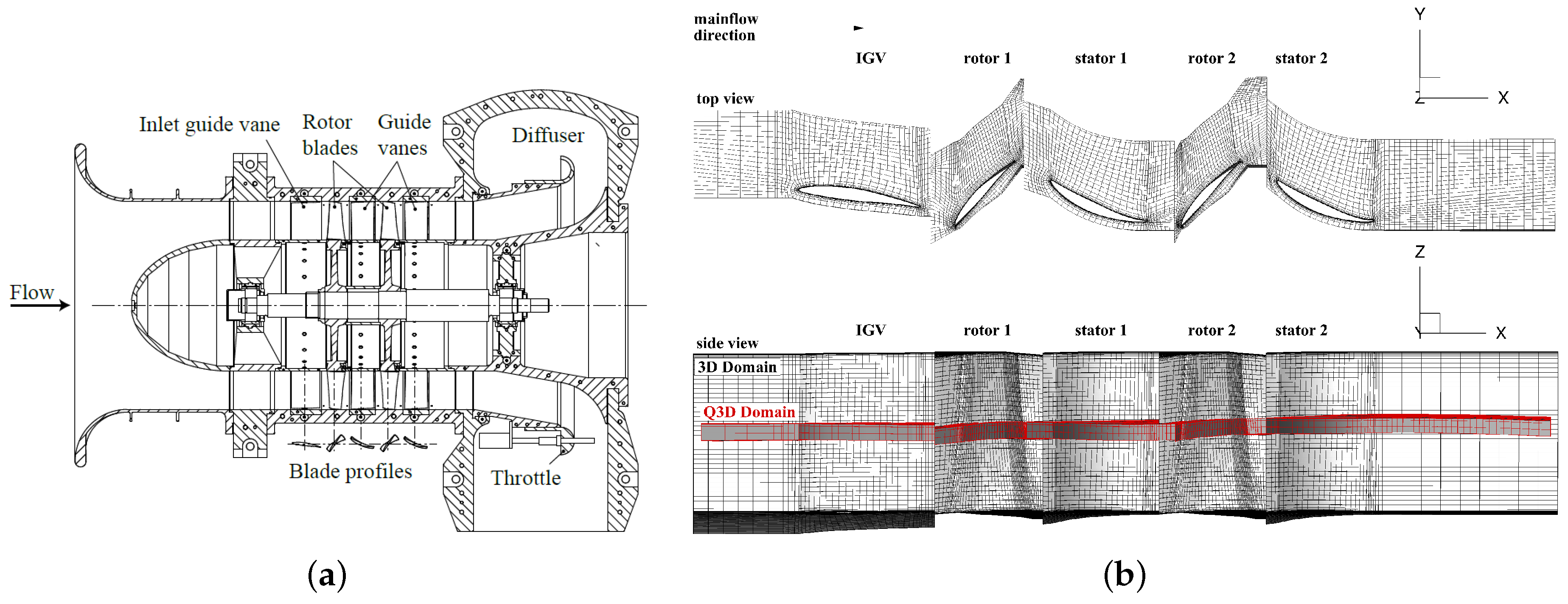
4. Low-Speed Axial Compressor Rig

Since the outlet flow of a cascade or a blade row is the inlet for the downstream blade row in a multistage environment, the accuracy of the upstream outlet flow is of major importance for multistage simulations. For this purpose, the low-speed axial compressor rig of the Institute of Turbomachinery and Fluid Dynamics at LU Hannover is used to undergo the next validation step with a more complex test-case where the focus is on wake-induced boundary layer transition.

Figure 5a gives a schematic overview of the low-speed axial compressor of the Institute of Turbomachinery and Fluid Dynamics. A detailed description of the test rig, the experimental data, and their underlying post-processing is given in Griebel and Seume [26]. Previous investigations showed the numerical prediction quality of the used CFD solver where the numerical method has been validated against experimental data in [27]. Wolff et al. [27] conducted steady and unsteady RANS simulations and showed that the first and last approximately 20% of the blade height are influenced by secondary flow effects. At midspan, a two dimensional flow can be assumed. Therefore, only 15% of the blade height at midspan are considered in quasi three-dimensional (Q3D) numerical simulations, cf. Figure 5b. Both measurements and numerical simulations have been conducted at steady state rotor speed of 3000 rpm for three different operating points. Furthermore, to take e.g., sidewall effects into account, the same axial velocity density ratio (AVDR) has been adjusted for the Q3D and the full 3D setup. In addition, the same mesh size and topology used by Wolff et al. is also used in the current work. Hence, the grid convergence study according to [28], which has been conducted by Wolff et al., remains valid. The results of the grid convergence study show a grid convergence index (GCI) for the used grid of GCI = 0.3% concerning the total pressure ratio and GCI = 3.13% concerning the isentropic efficiency. A detailed description of the conducted study can be found in [27]. Besides numerical simulations with the k-$\omega$-SST turbulence model [9] implemented in the version of 2003 [29] and coupled to the $\gamma$-Re_Θ transition model with the empirical correlations published by Langtry and Menter in 2009 [3] (SST), numerical simulations with the aforementioned VB model are conducted. The transitional behavior and the quality of its numerical prediction by the (U)RANS simulations are specified by means of both the ratio between isentropic thermal power circumferentially averaged at midspan and mechanical power output, calculated using the following equation

$${\eta }_{\mathrm{MTMS},\mathrm{is}}=\frac{\dot{m}{h}_{\mathrm{tot},1,\mathrm{m},\mathrm{MS}}({\Pi }_{\mathrm{tot},\mathrm{m},\mathrm{MS}}^{\frac{\kappa -1}{\kappa }}-1)}{P},$$

(8)

and experimental and numerically-determined space-time diagrams of the so called quasi wall shear-stress (QWSS). Thereby, the QWSS gained from the experimental data can be evaluated in the form:

$$QWSS=C{\tau }_w^{1/3}=\left(\frac{E^2-E_0^2}{E_0^2}\right),$$

(9)

where C is a calibration constant, ${\tau }_w$ is the wall shear-stress, E₀ is the anemometer voltage obtained under zero-flow conditions and E is the instantaneous output voltage from the anemometer.

4.1. Global Design Parameter

In Figure 6 the isentropic-to-mechanical efficiency ${\eta }_{\mathrm{MTMS},\mathrm{is}}$ is plotted as a function of the mass flow $\dot{m}$. The efficiency predicted by SST and VB for peak efficiency agrees the best with the measured efficiency where the VB gives a smaller mass flow compared to SST and the experimental data. Although there is a greater difference between the experimental data and the numerical results of near stall and near choke, they are also inside the measurement uncertainties. Nevertheless, it is apparent that VB predicts almost similar values for the isentropic-to-mechanical efficiency ${\eta }_{\mathrm{MTMS},\mathrm{is}}$ for near stall and peak efficiency, but tends to better predict the efficiency for the operating point near choke compared to SST.

4.2. Boundary Layer Behavior

The reason for the improved prediction of the efficiency of near choke can be seen in Figure 7. From the space-time diagrams of the QWSS gained from the experimental data (Figure 7a), it is clear that the vane experiences a laminar flow, which is alternately disturbed by a wake. The QWSS shows high values in the laminar region shortly downstream of the leading edge, which decrease to smaller values further downstream. The laminar flow is periodically disturbed by a wake, characterized by higher QWSS due to the higher turbulence intensity. At $x/l_{ax}>0.8$ the flow on the suction side is turbulent, because QWSS always shows a high value due to the higher turbulent viscosity relative to the laminar viscosity. A similar behavior can be seen in the space-time diagrams of the SST in Figure 7b and VB simulation in Figure 7c. Nevertheless, the numerical predicted wake seems to impinge on the suction side further downstream at $x/l_{ax}\approx 0.55$ and an open separation is predicted by both the SST and VB simulation. In spite of these differences, the extent of the wake-induced transition region predicted by VB is in better agreement with the experimental data. This leads to an increase in turbulent losses, a reduction of the isentropic-to-mechanical efficiency ${\eta }_{\mathrm{MTMS},\mathrm{is}}$ and, therefore, to a better agreement with the experimental data.

5. Conclusions

In this paper, an improved numerical method composed of the k-$\omega$ turbulence model after Wilcox (1988) [2] extended to incorporate turbulence length scale effects [10] in combination with the $\gamma$-Re_Θ transition model after Menter and Langtry [3] extended to three-dimensional cross-flow transition [7] (named herein VB) is validated in two turbine cascades with detailed experimental data on boundary layer state on suction and sidewall surfaces. The effect of prescribed turbulence length scales on the total pressure loss prediction at the outlet of the Durham cascade was shown. The improved numerical method (VB) was best in predicting total pressure loss compared to experimental data and also against numerical results from the SST turbulence model in combination with the transition model within the uncertainties of the overall Reynolds-Averaged Navier–Stokes approach and Boussinesq assumption. The reason for that is the better prediction of the secondary flow trajectory and hence, the interaction with the viscous regions on suction and sidewall surfaces as shown e.g., for the Langston cascade. Furthermore, the extension to three-dimensional boundary layer transition showed a local effect on the prediction of turbulent or at least transitional regions than on overall performance parameters like total pressure loss at the outlet of the Durham cascade. The effect of turbulence length scale on turbulence prediction and the influence on boundary layer and their transition to turbulence was emphasized in the multistage low-speed axial compressor rig. Here, the VB was again superior in prediction laminar-turbulent boundary layer transition and hence on the prediction efficiency. Finally, it can be concluded that the numerical method (VB and VB-CF) improves the prediction of turbulence and hence, boundary layer transition in two-dimensional and also three-dimensional steady and unsteady flows. The extension to cross-flow transition supports the local prediction of secondary flow phenomena and their interaction with the viscous regions but shows no effect (positive and negative) on overall performance parameters for the test-cases investigated here. The deficiencies regarding the quantitative prediction are a motivation for further modeling efforts to improve the prediction quality.

References

1. Denton, J.D. Some limitations of turbomachinery. In Proceedings of the ASME Turbo Expo 2010: Power for Land, Sea, and Air, Glasgow, UK, 14–18 June 2010. Paper No. GT2010-22540. [Google Scholar]
2. Wilcox, D.C. Reassesment of the scale-determining equation for advanced turbulence models. AIAA J. 1988, 26, 1299–1310. [Google Scholar] [CrossRef]
3. Langtry, R.B.; Menter, F.R. Correlation-Based Transition Modeling for Unstructured Parallelized Computational Fluid Dynamics Codes. AIAA J. 2009, 47, 2894–2906. [Google Scholar] [CrossRef]
4. Bode, C.; Aufderheide, T.; Friedrichs, J.; Kožulović, D. Improved Turbulence and Transition Prediction for Turbomachinery Flows. In Proceedings of the ASME 2014 International Mechanical Engineering Congress and Exposition, Montreal, QC, Canada, 14–20 November 2014. Paper No. IMECE2014-36866. [Google Scholar]
5. Holley, B.M.; Becz, S.; Langston, L.S. Measurement and calculation of turbine cascade endwall pressure and shear stress. In Proceedings of the ASME Turbo Expo, Reno-Tahoe, NV, USA, 6–9 June 2005. Paper No. GT2005-68256. [Google Scholar]
6. Denton, J.D.; Pullan, G. A Numerical Investigation into the Sources of Endwall Loss in Axial Flow Turbines. In Proceedings of the ASME Turbo Expo 2012: Turbine Technical Conference and Exposition, Copenhagen, Denmark, 11–15 June 2012. Paper No. GT2012-69173. [Google Scholar]
7. Bode, C.; Friedrichs, J.; Kožulović, D. Abschlussbericht zum LuFo IV/4 GTF-Turb; Technical Report; Institut für Flugantriebe und Strömungsmaschinen, Technische Universität Braunschweig: Braunschweig, Germany, 2016. [Google Scholar]
8. Menter, F.R.; Smirnov, P.E. Development of a RANS-based Model for Predicting Crossflow Transition. In Proceedings of the Contributions to the 19th STAB/DGLR Symposium, München, Germany, 4–5 November 2014. [Google Scholar]
9. Menter, F.R. Two-Equation Eddy-Viscosity Turbulence Models for Engineering Applications. AIAA J. 1994, 32, 1598–1605. [Google Scholar] [CrossRef]
10. Bode, C.; Aufderheide, T.; Kožulović, D.; Friedrichs, J. The Effects of Turbulence Length Scale on Turbulence and Transition Prediction in Turbomachinery Flows. In Proceedings of the ASME 2014 Turbine Technical Conference and Exposition, Düsseldorf, Germany, 16–20 June 2014. Paper No. GT2014-27026. [Google Scholar]
11. Marciniak, V.; Kügeler, E.; Franke, M. Predicting Transition on Low-Pressure Turbine Profiles. In Proceedings of the V European Conference on Computational Fluid Dynamics ECCOMAS CFD 2010, Lisbon, Portugal, 14–17 June 2010. [Google Scholar]
12. Kato, M.; Launder, B.E. The Modelling of Turbulent Flow Around Stationary and Vibrating Square Cylinders. In Proceedings of the Ninth Symposium on Turbulent Shear Flows, Kyoto, Japan, 16–18 August 1993. [Google Scholar]
13. Arnal, D.; Habiballah, C.; Coustols, C. Laminar instability theory and transition criteria in two- and three-dimensional flows. La Recherche Aerospatiale 1984, 2, 45–63. [Google Scholar]
14. Menter, F.R.; (ANSYS, Otterfing, Germany). Private communication, 2015.
15. Durbin, P.A. On the k-epsilon Stagnation Point Anomaly. Int. J. Heat Fluid Flow 1996, 17, 89–90. [Google Scholar] [CrossRef]
16. Kožulović, D. Modellierung des Grenzschichtumschlags bei Turbomaschinenströmungen unter Berücksichtigung mehrerer Umschlagsarten. Ph.D. Thesis, Ruhr-Universität Bochum, Bochum, Germany, 2007. [Google Scholar]
17. Vera, M.; de la Rosa Blanco, E.; Hodson, H.; Vazquez, R. Endwall boundary Layer development in an engine representative four-stage low pressure turbine rig. J. Turbomach. 2008, 131, 011017. [Google Scholar] [CrossRef]
18. Moore, H.; Gregory-Smith, D.G. Transition effects on secondary flows in a turbine cascade. In Proceedings of the ASME 1996 International Gas Turbine and Aeroengine Congress and Exhibition, Birmingham, UK, 10–13 June 1996. Paper No. 96-GT-100. [Google Scholar]
19. Holley, B.M.; Langston, L.S. Surface Shear Stress and Pressure Measurements in a Turbine Cascade. J. Turbomach. 2009, 131, 031014. [Google Scholar] [CrossRef]
20. Cui, J.; Rao, V.N.; Tucker, P. Numerical Investigation of Contrasting Flow Physics in Different Zones of a High-Lift Low-Pressure Turbine Blade. J. Turbomach. 2016, 138, 011003. [Google Scholar] [CrossRef]
21. Schlichting, H.; Gersten, K. Grenzschicht-Theorie; Springer: Berlin/Heidelberg, Germany, 2006. [Google Scholar]
22. Walsh, J.G.C. Secondary Flows and Inlet Skew in Axial Flow Turbine Cascade. Ph.D. Thesis, School of Engineering and Computer Sciences, The University of Durham, Durham, UK, 1987. [Google Scholar]
23. Moore, H. Experiments in a Turbine Cascade for the Validation of Turbulence and Transition Models. Ph.D. Thesis, School of Engineering and Computer Sciences, University of Durham, Durham, UK, 1995. [Google Scholar]
24. Langston, L.S.; Nice, M.L.; Hooper, R.M. Three-Dimensional Flow Within a Turbine Cascade Passage. J. Eng. Power 1977, 99, 21–28. [Google Scholar] [CrossRef]
25. Graziani, R.A.; Blair, M.F.; Taylor, J.R.; Mayle, R.E. An Experimental Study of Endwall and Airfoil Surface Heat Transfer in a Large Scale Turbine Blade Cascade. ASME J. Eng. Power 1980, 102, 257–267. [Google Scholar] [CrossRef]
26. Griebel, A.; Seume, J.R. The Influence of Variable Rotor-Stator Interaction on Boundary-Layer Development in an Axial Compressor. In Proceedings of the ASME Turbo Expo 2005: Power for Land, Sea, and Air, Reno, NV, USA, 6–9 June 2005. Paper No. GT2005-68902. [Google Scholar]
27. Wolff, T.; Herbst, F.; Freund, O.; Liu, L.; Seume, J.R. Validating the Numerical Prediction of the Aerodynamics of an Axial Compressor. In Proceedings of the ASME Turbo Expo 2014: Turbine Technical Conference and Exposition, Düsseldorf, Germany, 16–20 June 2014. Paper No. GT2014-25530. [Google Scholar]
28. ASME Performance Test Codes Comitee Standard for Verification and Validation in Computational Fluid Dynamics and Heat Transfer; Technical Report ASME V&V 20-2009; The American Society of Mechanical Engineers: New York, NY, USA, 2009.
29. Menter, F.R.; Kuntz, M.; Langtry, R.B. Ten Years of Industrial Experience with the SST Turbulence Model. In Turbulence, Heat and Mass Transfer 4; Hanjalic, K., Nagano, Y., Tummers, M., Eds.; Springer Verlag: Berlin, Germany, 2003. [Google Scholar]
30. Bode, C.; Friedrichs, J.; Müller, C.; Herbst, F. Application of Crossflow Transition Criteria to Local Correlation-Based Transition Model. In Proceedings of the Propulsion and Energy Forum, 52nd AIAA/SAE/ASEE Joint Propulsion Conference, Salt Lake City, UT, USA, 25–27 July 2016. [Google Scholar]
Figure 1. Pitchwise averaged spanwise distributions at slot 10 compared to Figure 5 in [7]. (a) Effect of turbulence length scale lT; (b) Effect of crossflow extension (CF), lT = 9.4 mm.
Ijtpp 03 00018 g001
Figure 2. Comparison of numerical predicted intermittency γ e f f , d i f f ( γ e f f according to the original γ -ReΘ transition model [3]) with (VB-CF) and without (VB) cross-flow extension. (a) Sidewall; (b) Suction side.
Ijtpp 03 00018 g002
Figure 3. Comparison between experimental [19] and numerical results for surface pressure coefficient c p of the Langston Cascade.
Ijtpp 03 00018 g003
Figure 4. Comparison between experimental [19] and numerical results for surface pressure coefficient c p as well as skin friction coefficient cf c f × 10 3 isolines on the sidewall of the Langston Cascade.
Ijtpp 03 00018 g004
Figure 5. Schematic overview and computational domain of the Low-Speed Axial Compressor. (a) Schematic overview; (b) Computational domain. IGV: Inlet Guide Vane.
Ijtpp 03 00018 g005
Figure 6. Isentropic-to-mechanical efficiency η MTMS , is over mass flow m ˙ for all three operating points, circumferential-averaged at midspan.
Ijtpp 03 00018 g006
Figure 7. Space-Time Diagrams of quasi wall shear-stress (QWSS) on the Suction Side for the “near choke” condition.
Ijtpp 03 00018 g007