Optimization of the LS89 Axial Turbine Profile Using a CAD and Adjoint Based Approach ^†

Abstract

The LS89 high pressure axial turbine vane was originally designed and optimized for a downstream isentropic Mach number of 0.9. This profile has been widely used for computational fluid dynamics (CFD) validation in the open literature but very few attempts have been made to improve the already optimized design. This paper presents a sound methodology to design and optimize the LS89 using computer-aided design (CAD) at design conditions. The novelty of the study resides in the parametrization of design space, which is done at the CAD level, and the detailed analysis of the aerodynamic performance of the optimized design. Higher level constraints are imposed on the shape, such as the trailing edge thickness, the axial chord length, and G2 geometric continuity between the suction side and pressure side at the leading edge. The gradients used for the optimization are obtained by applying algorithmic differentiation to the CAD kernel and grid generator and the discrete adjoint method to the CFD solver. A reduction of almost 12% entropy generation is achieved, which is equivalent to a 16% total pressure loss reduction. The entropy generation is reduced while keeping the exit flow angle as a flow constraint, which is enforced via the penalty formulation. The resulting unconstrained optimization problem is solved by the L-BFGS-B algorithm. The flow is governed by the Reynolds-averaged Navier-Stokes equations and the one-equation transport Spalart-Allmaras turbulence model. The optimal profile is compared and benchmarked against the baseline case.

1. Introduction

Designing and optimizing a turbine vane is a complex iterative design process that can take significant time and effort. The use of relatively low-cost numerical shape optimization methods has become more popular and have been widely used in turbomachinery applications. In particular, the adjoint method enables the efficient computation of the sensitivities required by gradient-based optimizers, at a cost independent of the number of design variables [1].

Typically, the grid point coordinates have been used as design variables [2]. This approach offers a very rich design space but has some drawbacks that need to be considered. First, the connection to the computer-aided design (CAD) geometry is lost. This means that an additional step is required to transform the optimal shape defined by grid points back to smooth CAD shape. Secondly, although there are several successful methods that can be used to convert a cloud of grid points to CAD [3,4], the fitting error can impair the optimality of the shape. Furthermore, this additional step can take significant time and it is not guaranteed that the final approximated CAD shape will meet the design requirements and constraints [5,6]. Also, the use of a smoother is inevitable to avoid irregular shapes. To avoid these problems, in this study it is proposed to keep the CAD geometry in the optimization loop.

The advantage of including the CAD model in the design system is that higher level constraints can be imposed on the shape, allowing the optimized model or component to be manufactured. Additionally, the adjoint sensitivities are automatically filtered and only smooth shapes can be produced. One of the limitations of using the CAD in a gradient-based optimization framework is the computation of the grid sensitivities i.e., the partial derivative of the grid points with respect to the design parameters. These sensitivities can be approximated by finite differences using the design velocity approach [7], which is robust against the possible changes in boundary topology of the model. However, this approach is based on computing shape differences between two surface meshes and can introduce issues of surface to surface projection when computing the distances between the two surface meshes. Moreover, finite differences inaccuracies are introduced in the design velocity approach because of the limited arithmetic precision if the step size is too small and the truncation error if the step size is too big. The use of inaccurate sensitivities can slow the convergence of the optimizer. This work aims to circumvent these issues by making use of algorithmic differentiation (AD) [8] for the CAD kernel and the grid generation [9]. Algorithmic differentiation allows to compute the derivatives of an output of a program with respect to the inputs by applying the chain rule in an automatic fashion throughout the evaluation of the code. This means that the grid sensitivities will be accurate to machine accuracy.

In this study, it is proposed to use a CAD-based adjoint-based optimization method for the LS89 [10,11] high pressure axial turbine nozzle guide vane profile. The LS89 was originally designed and optimized at the Von Karman Institute for Fluid Dynamics for a subsonic isentropic outlet Mach number of 0.9 by the inverse method [11], which is an iterative design method based on both potential and Euler type solvers that uses the difference between the calculated velocity distribution and the required one to modify the profile geometry. Montanelli et al. [12] performed both single-point and multi-point optimizations on the LS89 to reduce the total pressure losses by constraining the outlet mass flow, while keeping the leading edge (LE) and trailing edge (TE) geometries and the profile thicknesses fixed and using the L-BFGS-B algorithm to explore different geometries with a wing parametrization model. This group also solved the Reynolds-Averaged Navier-Stokes (RANS) equations and the one-equation transport Spalart-Allmaras turbulence model and computed the gradients assuming that the eddy viscosity and thermal conductivity are constant. They achieved a total pressure loss reduction below 1% for the nominal case (outlet $M_{ise}$ = 0.927). The question arises whether the LS89 is indeed optimal, and if it could be optimized further. This paper addresses this and presents an adjoint optimization of the turbine profile, by using a novel CAD-based approach in which:

• The optimal shape remains defined within the CAD tool. The optimization problem herein is expressed by CAD parameters that are directly used in defining the CAD geometry by means of Bézier and B-spline curves.
• The in-house CAD and grid generation tools are automatically differentiated in forward mode to obtain the exact derivatives of the grid coordinates with respect to the CAD-based design parameters. This allows for an accurate prediction of the sensitivities and circumvention of the errors introduced by finite differences.
• The trailing edge thickness and axial chord length are kept fixed as manufacturing constraints and the exit flow angle is considered as an aerodynamic constraint.

A computer aided design and optimization tool for turbomachinery applications (CADO) [13] is used throughout this study.

2. Computer-Aided Design-Based Parametrization

The construction of the turbine profile shown in Figure 1 is based on the parametrization described by [14]. The profile is defined by a set of CAD-based or engineering-based design parameters that are relevant to the aerodynamic performance (e.g., solidity, stagger angle, etc.) and the manufacturing requirements (e.g., axial chord length, trailing edge radius). First, a camber line is constructed. The points $P_{LE}$, $P_{mid}$, $P_{TE}$ define the control points of the 2nd order Bézier curve describing the camber line. The camber line is used to define the position of the control points of the suction side (SS) and pressure side (PS) B-spline curves relative to it. The profile is constructed by two B-spline curves for the SS and PS and a circular arc at the trailing edge (TE) to close the profile. The normal distance of the first control point relative to the camber line is calculated in such a way that G2 geometric continuity (i.e., equal curvature) is maintained between the SS and PS B-splines at the leading edge.

3. Optimization

The purpose of the optimization algorithm (Figure 2) is to reduce the entropy generation $J_1$ (Equation (1)) while maintaining the exit flow angle $J_2$ (Equation (2)) above or equal to the baseline value of $J_{2,ref}=74.83$ deg, by modifying the design vector $\overrightarrow{\alpha }$. The flow state $\overrightarrow{U}$ and the design vector $\overrightarrow{\alpha }$ are coupled via the primal flow governing equations. The constrained optimization problem is handled with the penalty method. The penalty term becomes active only when the exit flow angle is below the target value. The $J_{2,flag}$ parameter is either set to 1.0 or 0.0 in order to activate or deactivate the penalty term respectively. The weighed cost function of the single point $J_{SP}$ optimization problem is given by Equation (3). The L-BFGS-B algorithm [15] available in the Python SciPy package [16] is used to find the new design vector.

$$J_1(\overrightarrow{\alpha },\overrightarrow{U})=\frac{{\int }_{out}p{\rho }^{1-\gamma }{V}_{x}dy}{{\dot{m}}_{out}}$$

(1)

$$J_2(\overrightarrow{\alpha },\overrightarrow{U})=atan\left(\frac{\overline{V_y}}{\overline{V_x}}\right)$$

(2)

$$J_{SP}(\overrightarrow{\alpha },\overrightarrow{U})=\frac{J_1}{J_{1,ref}}+J_{2,flag}{J}_{2,coef}{\left(\frac{J_2}{J_{2,ref}}-1\right)}^2$$

(3)

3.1. Grid Generation

A multi-block structured grid is generated for every optimization iteration. A mesh-independence study was carried out in order to select an appropriate mesh for the optimization. One O-grid block is placed around the profile and there are six additional H-grid blocks, four of them distributed around the profile and the remaining two being used as the inlet and outlet blocks. Torreguitart et al. [9] describe in more detail how the grid was generated.

3.2. Flow and Adjoint Solvers

The flow solver employs a cell-centered finite volume discretization on multiblock structured grids. The three dimensional compressible RANS equations are solved with an implicit time integration scheme accelerated by local time-stepping and multigrid. The fluid is considered as a calorically perfect gas and the eddy-viscosity hypothesis is used to account for the effect of turbulence. Convective fluxes are computed using Roe’s approximate Riemann solver [17] with a monotonic upstream-centered scheme for conservation laws (MUSCL)-type reconstruction [18] of primitive variables to attain second order accuracy. Oscillations near shocks are suppressed by a van-Albada type limiter [19]. The numerical dissipation of the scheme is controlled by the entropy correction by Harten and Hyman [20] for both linear and non-linear eigenvalues. Viscous fluxes are calculated with a central discretization scheme, while the negative Spalart-Allmaras turbulence model [21] is used for the turbulence closure problem assuming fully turbulent flow from the inlet ($R{e}_{inlet}\approx 2\times {10}^5$). Boundary conditions are imposed weakly by utilizing the dummy cell concept [22]. The hand derived discrete adjoint solver uses constant eddy viscosity assumption which is a valid approach for engineering design applications. The flow solver and its discrete adjoint counterpart use the stabilization scheme described by [23].

3.3. Gradient Computation

Torreguitart et al. [9] showed the first results of differentiating the CAD kernel and grid generation tools using the AD tool Automatic Differentiation by OverLoading in C++ (ADOL-C) [24]. In the work herein, the optimization algorithm computes the grid sensitivities $d\overrightarrow{X}/d\overrightarrow{\alpha }$ for every optimization step, using the forward vector mode as opposed to the forward scalar or reverse modes as it allows to compute $d\overrightarrow{X}/d\overrightarrow{\alpha }$ in one single evaluation of the primal at a relatively low cost.

The performance sensitivities $dJ/d\overrightarrow{\alpha }$ for each cost function $J_1$ or $J_3$ are computed by doing a scalar product of the adjoint calculated sensitivities $dJ/d\overrightarrow{X}$ (i.e., the derivative of the cost function with respect to the grid coordinates $\overrightarrow{X}$) with the grid sensitivities $d\overrightarrow{X}/d\overrightarrow{\alpha }$. A suitable step-size for each design variable was selected to compute the gradients with finite differences and compare them against the gradients obtained by the discrete adjoint. Figure 3 shows a good agreement with finite differences for both the entropy generation and exit flow angle. The largest sensitivities shown in Figure 3 correspond to the design variables ${\alpha }_j$ = 1 ($c_{ax}$) and 4 ($R_{TE}$), which do not change during the optimization because they are considered manufacturing constraints.

4. Results

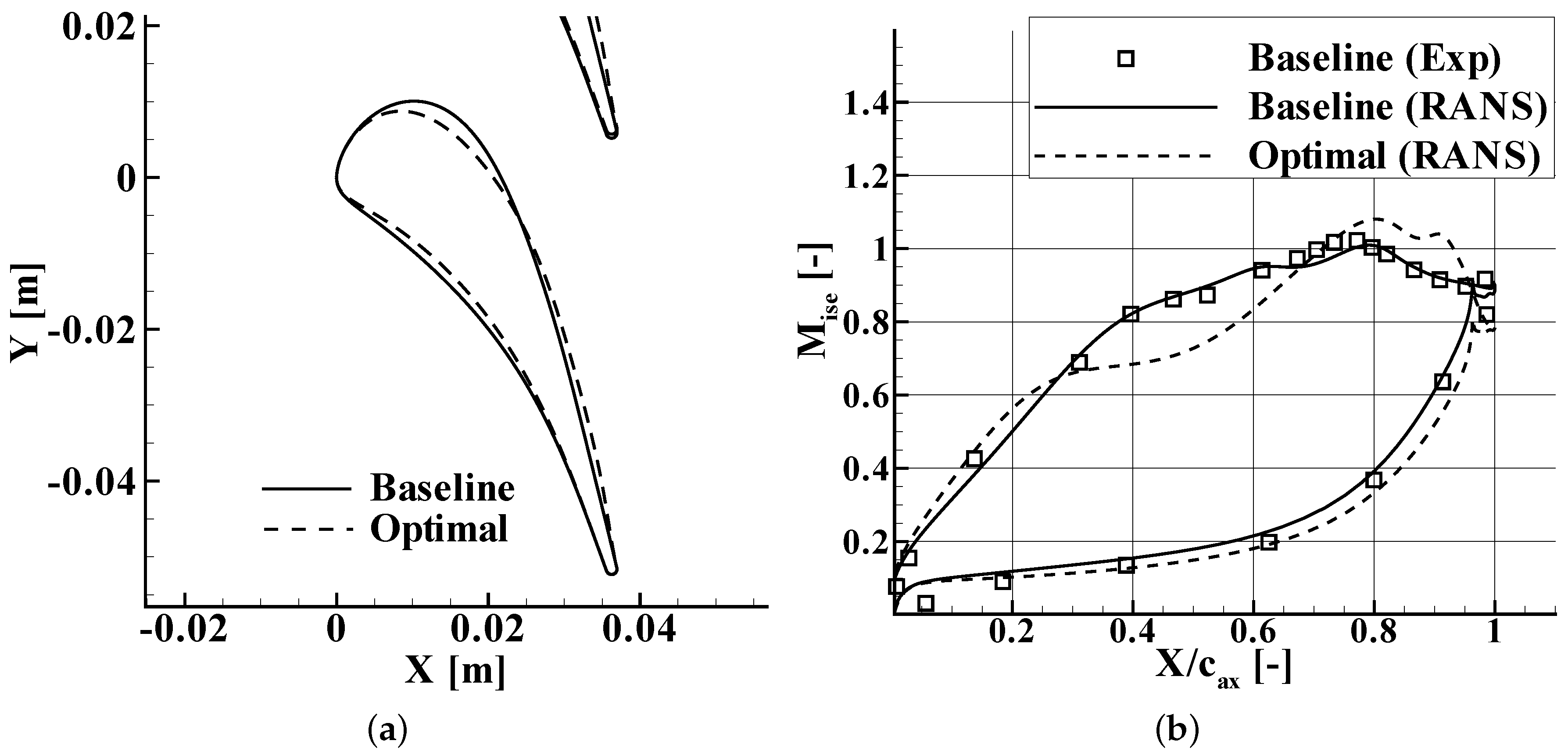
Figure 4a shows significant shape differences between the baseline and the optimal shape, the latter being a more aft-loaded profile than the baseline design. The isentropic Mach number distributions are shown in Figure 4b, which shows a fairly good agreement between the $M_{ise}$ predicted by CFD and the experimental data (MUR45 test condition, with downstream $M_{ise}=0.875$, see [10]) for the baseline geometry.

The L-BFGS-B algorithm converges within 20 optimization iterations. More cycles were performed but no further decrease in the objective function was obtained. Despite the fact that the mass flow for the optimal geometry has increased slightly by 1.2%, the entropy generation is reduced by 11.6%, while maintaining the exit flow angle within ±0.1% of the baseline value. As the aft-loaded profile has significant rear suction side curvature, the flow is rapidly accelerated towards a higher peak Mach number than the baseline design. This is followed by a deceleration from $X/c_{ax}$ = 0.8 to 0.88 and a small acceleration from $X/c_{ax}$ = 0.88 to 0.91. At $X/c_{ax}$ = 0.91 the flow is rapidly decelerated again and leaves the trailing edge at a significantly lower exit isentropic Mach number. The strong deceleration towards the end of the suction side suggests that the boundary layer will be thicker and one would expect higher profile losses.

The total pressure loss reduction between the inlet and the fully mixed-out flow at the outlet plane, expressed via $P_{01}-P_{02}$ or by the ${\zeta }_2$ coefficient (see Equation (4)), is of the order of 16.3%.

The downstream total pressure loss profile, at the plane $X/c_{ax}=1.433$, is shown in Figure 5. In the vertical axis the total pressure loss $P_{01}-P_{0X}$ between the inlet and a downstream plane at $x/c_{ax}=1.433$ is expressed as a a percentage of the downstream dynamic head $q_X$ at the $X/c_{ax}=1.433$ plane. This figure shows that the total pressure loss generated in the wake is reduced significantly.

To understand why the optimal shape is more efficient than the baseline, the following subsections will look into the loading, boundary layer parameters, base pressure and profile losses for each profile.

$$\begin{array}{c}\hfill {\zeta }_2=1-{\displaystyle \frac{1-{({\displaystyle \frac{p_2}{P_{02}}})}^{{\displaystyle \frac{\gamma -1}{\gamma }}}}{1-{({\displaystyle \frac{p_2}{P_{01}}})}^{{\displaystyle \frac{\gamma -1}{\gamma }}}}}\end{array}$$

(4)

4.1. Zweifel Loading Coefficient

The total loading, which can be expressed as the integral of the $p_{PS}-p_{SS}$ over the axial chord length, has increased by 1% for the optimal shape as a result of the 1% increase in the pitch and having the same exit flow angle. The Zweifel loading coefficient $Z_w$ [25] is a measure of how efficiently the profile is loaded. An efficient loaded profile would be one in which the pressure is stagnated over the pressure side and the velocity on the suction side is constant and equal to the downstream velocity. The Zweifel’s design rule says that loss is minimized for $0.8<Z_w<1$. Equation (5) was used to calculate the Zweifel loading coefficient, which increased from 0.636 for the baseline to 0.646 for the optimal.

$$\begin{array}{c}\hfill Z_w=\frac{{\int }_0^1(p_{PS}-p_{SS})\frac{dx}{c_{ax}}}{(P_{01}-p_2)c_{ax}}\end{array}$$

(5)

4.2. Boundary Layer Parameters

The state of the boundary layer close to the trailing edge is deemed to have an impact on the profile losses (see Equation (6)).

Table 1. Boundary layer parameters.

	Units	Baseline at ${\mathit{M}}_{\mathit{ise},\mathit{max}}$	Optimal at ${\mathit{M}}_{\mathit{ise},\mathit{max}}$	Baseline at ${\mathit{X}}_{\mathit{SS},\mathit{TE}}$	Optimal at ${\mathit{X}}_{\mathit{SS},\mathit{TE}}$
$\delta /D_{TE}$	[-]	0.501	0.390	0.939	1.11
${\delta }^{*}/D_{TE}$	[-]	0.104	0.079	0.206	0.346
$\theta /D_{TE}$	[-]	0.0557	0.0405	0.1186	0.1780
H	[-]	1.86	1.96	1.74	1.95

compares the boundary layer parameters between the baseline and optimal shapes for two locations on the suction side: at the peak $M_{ise}$ location and very close to the TE (approximately at $x=0.03$ m and $x=0.037$ m respectively, see Figure 4b). The latter location is defined herein as the point of the suction side slightly upstream of the TE circle. The boundary layer velocity profiles are shown in Figure 6 for both locations, showing that there is no boundary layer separation.

At the peak $M_{ise}$ location, the boundary layer thickness $\delta$ for the optimal design is smaller than for the baseline, as expected due to the higher acceleration. When the flow decelerates from the peak $M_{ise}$ location to the point just upstream of the trailing edge circle, the boundary layer thickness almost doubles for the baseline and triples for the optimal profile. The resulting $\delta$ of the optimal shape is 18% thicker than the baseline. The shape factor H is higher for the optimal than for the baseline design in both locations, which means that the optimal profile has stronger adverse pressure gradient. The shape factor for both designs are between the typical laminar Blasius boundary layer value ($H=2.59$) and the turbulent values (H = 1.3–1.5).

From a boundary layer perspective, the optimal design would have higher profile losses due to the higher thickness displacement and momentum thickness. However, there is at least one more factor to be considered when determining the profile losses: the base pressure.

4.3. Base Pressure

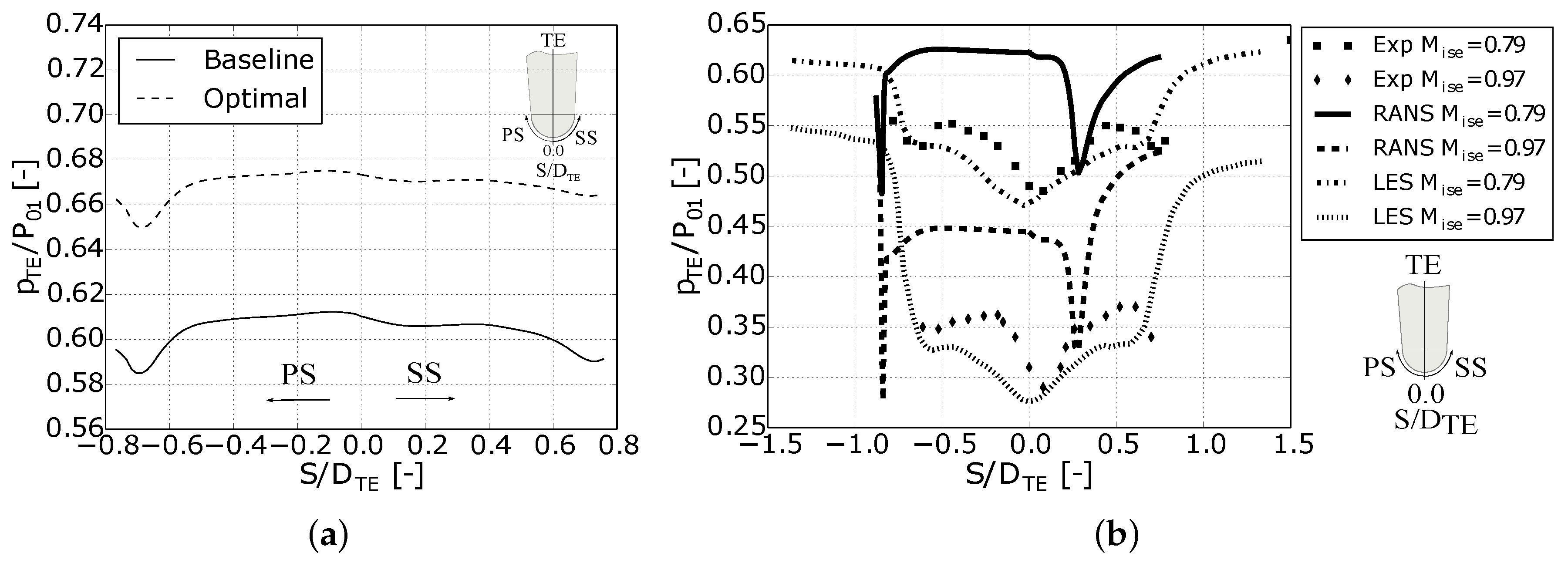
The base pressure, which is the static pressure at the mid point of the trailing edge, is known to play an important role in the profile losses. Higher base pressures contribute to the reduction of the profile losses. The trailing edge pressure distribution shown in Figure 7a shows that the optimal shape has a 10% higher base pressure. It is generally thought that higher values of boundary layer thickness result in higher values of base pressure [26]. Higher base pressures are expected of an aft-loaded profile with significant rear suction side curvature and higher values of unguided or uncovered turning [27]. The angle between tangents to blade suction side in the throat and at the TE increased by 6.76 degrees when going from the baseline to the aft-loaded optimal profile. According to the base pressure correlation given by Sieverding et al. [27], the optimal profile is expected to have 3% higher base pressure than the baseline. The percentage increase predicted by the correlation is mainly due to the higher suction side rear curvature because the trailing edge wedge angle difference between the baseline and optimal profiles is negligible. However, Sieverding et al. [27] also showed that, for 80% of the tested blades, there was a discrepancy between the predicted base pressures (using the correlation) and the measured ones of the order of ±5% of the downstream pressure. Although there are no measurements available for the optimal profile yet, by taking this error into account the minimum and maximum values for the base pressure of the optimal profile can be estimated to be 5% lower and 16.7% higher than the baseline respectively. The RANS prediction for the base pressure falls inside this range, since the base pressure of the optimal design is predicted to be 10% higher than the baseline. However, only unsteady analysis and experimental tests will be able to provide enough evidence to support these results.

Predicting the absolute values of the base pressure correctly can be very difficult due to the highly complex nature of the flow in the trailing edge. Vagnoli et al. [29] showed that steady state simulations usually predict the wrong shape or distribution of pressure around the trailing edge, whereas large eddy simulation (LES) or Unsteady Reynolds-Averaged Navier-Stokes (URANS) capture much better the shape and the pressure values when compared to experimental data. The pressure distribution shown in Figure 7a is a nearly-uniform pressure around the trailing edge, which is suspected to be different to the real pressure distribution profile. However, it is believed that the base pressure delta difference between two steady state simulations, one for the optimal and the other for the baseline profiles, is a fairly good estimate of the real difference. The validity of this assumption has been investigated by performing two RANS simulations for the turbine profile that was tested by [28] at $M_{ise}=0.79$ and $0.97$ and comparing the base pressure delta between these two operating conditions against the experimental data and the LES results performed by [29] (Figure 7b). The base pressure delta, which is taken at $S/D_{TE}=0$ from Figure 7b, is 0.18 for both the experiments and RANS and 0.20 for LES. This confirms that, despite the limitations of CFD in predicting the base pressure absolute values, RANS is able to capture very well the relative differences in base pressure between two operating conditions.

4.4. Profile Losses

Denton et al. [30] showed that the profile losses for incompressible flow can be related to the base pressure coefficient and the boundary layer parameters, as shown in Equation (6). The relative effect of the base pressure coefficient is increased in compressible flow [31]. For blades operating in the transonic range from 0.8 to 1.2 the major source of loss is the trailing edge loss at these speeds and the base pressure plays a dominant role in determining the loss [26]. The profile loss split is shown in

Table 2. Profile loss contribution for the baseline and optimal.

	Units	Baseline	Optimal	Variation
$\frac{-C_b{D}_{TE}}{t}$	[-]	−0.0016	−0.0065	302.2%
$2\frac{{\theta }_{SS}+{\theta }_{PS}}{t}$	[-]	0.0066	0.0095	43.5%
${\left(\frac{{\delta }_{SS}^{*}+{\delta }_{PS}^{*}+D_{TE}}{t}\right)}^2$	[-]	0.0010	0.0012	21%
${\zeta }_p$	[-]	0.0060	0.0042	−30%

. The higher ${\delta }^{*}$ and $\theta$ values of the optimal shape contribute to increasing the profile loss. However, the reduction in profile losses due to the 302.2% increase in the trailing edge loss term dominates and explains the overall 30% reduction in profile losses. Still, if the base pressure increase was equal or below 6.54%, the optimal shape would have similar or higher profile losses than the baseline, respectively. The question arises whether using RANS for the optimization of an axial turbine operating at transonic speeds is a valid approach, since the base pressure plays such a dominant effect on the profile losses for such speeds and the flow field around the TE of a transonic turbine blade is too complex to be captured by RANS. Future LES simulations and or experimental tests are going to be necessary to support or reject the aerodynamic improvements reported herein for the optimal shape.

$$\begin{array}{c}\hfill {\zeta }_p=\frac{-C_b{D}_{TE}}{t}+2\frac{{\theta }_{SS}+{\theta }_{PS}}{t}+{\left(\frac{{\delta }_{SS}^{*}+{\delta }_{PS}^{*}+D_{TE}}{t}\right)}^2\end{array}$$

(6)

4.5. Off-Design Performance

The 16% reduction in total pressure loss shown in

Table 3. Comparison between the baseline and optimal.

	Acronyms	Units	Baseline	Optimal	Variation
Entropy generation	$J_1$	[Pa/(kg/m3)]	826.7	731.0	−11.6%
Exit flow angle	$J_3$	[deg]	74.89	74.89	−0.01%
Mass flow	$\dot{m}$	[kg/s]	0.008	0.009	+1.2%
Total pressure losses	$P_{01}-P_{02}$	[kPa]	2.47	2.07	−16.3%
Downstream loss coeff	${\zeta }_2$	[-]	0.02986	0.02500	−16.3%
Profile losses	${\zeta }_p$	[-]	0.0060	0.0042	−30%
Zweifel coefficient	$Z_w$	[-]	0.67	0.81	+21.2%
Solidity	$\sigma$	[-]	1.118	1.108	−0.9%
Pitch	g	[m]	0.0575	0.0580	+0.9%

was achieved for an outlet isentropic Mach number of 0.9 while keeping the axial chord length and trailing edge radius fixed and exit flow angle above 74.83 deg. However, the performance of the optimal profile is deemed to deteriorate significantly at off-design conditions. Figure 8 shows the total pressure loss coefficient for different outlet isentropic Mach numbers for the baseline and optimal profiles, which is defined as the total pressure difference between the inlet and outlet divided by the dynamic head at the outlet plane. At off-design conditions, the aerodynamic improvements of the optimal are reduced as the downstream isentropic Mach number is increased. Beyond $M_{ise,2}=0.94$, the baseline would have lower total pressure losses than the optimal profile. A detailed aerodynamic performance study of the baseline and optimal geometries at off-design conditions is outside the scope of this work but can be found in the multi-point optimization study carried out by Torreguitart et al. [32], where the performance of the LS89 is significantly improved at off-design conditions.

5. Conclusions

This paper presents an single point optimization of the LS89 axial turbine cascade vane profile for the design downstream isentropic Mach number of 0.9. The parameterization is done at the CAD level, which allows the imposition of higher level constraints on the shape, such as the axial chord length, the trailing edge radius and G2 geometric continuity between the suction side and pressure side at the leading edge. Additionally, the adjoint sensitivities are filtered out and only smooth shapes are produced. The use of algorithmic differentiation for the CAD kernel and grid generator allows computing the grid sensitivities to machine accuracy and avoid the limited arithmetic precision and the truncation error of finite differences. The optimization results show that the total pressure losses and entropy generation can be reduced by 16% and nearly 12% respectively by going from a front to a rear loaded profile and by keeping the exit flow angle fixed. Despite the increase in mass flow, loading, boundary layer thickness displacement and momentum thickness, the base pressure coefficient plays a dominant role herein and reduces the profile losses by 30%. The substantial aerodynamic improvements reported have not been observed previously, probably due to the fact that the current CAD-based parametrization allowed the exploration of a richer design space. The relative delta in base pressure predicted by the steady simulation between the optimal and baseline profiles is deemed to be representative of the real value, as RANS tends to capture well the relative differences between two designs. However, future unsteady studies or experimental investigations would be beneficial in order to confirm these findings.