One-Dimensional Annular Diffuser Model for Preliminary Turbomachinery Design

Abstract

Annular diffusers are frequently used in turbomachinery applications to recover the discharge kinetic energy and increase the total-to-static isentropic efficiency. Despite its strong influence on turbomachinery performance, the diffuser is often neglected during the preliminary design. In this context, a one-dimensional flow model for annular diffusers that accounts for the impact of this component on turbomachinery performance was developed. The model allows use of arbitrary equations of state and to account for the effects of area change, heat transfer, and friction. The mathematical problem is formulated as an implicit system of ordinary differential equations that can be solved when the Mach number in the meridional direction is different than one. The model was verified against a reference case to assess that: (1) the stagnation enthalpy is conserved and (2) the entropy computation is consistent and it was found that the error of the numerical solution was always smaller than the prescribed integration tolerance. In addition, the model was validated against experimental data from the literature, finding that deviation between the predicted and measured pressure recovery coefficients was less than 2% when the best-fit skin friction coefficient is used. Finally, a sensitivity analysis was performed to investigate the influence of several input parameters on diffuser performance, concluding that: (1) the area ratio is not a suitable optimization variable because the pressure recovery coefficient increases asymptotically when this variable tends to infinity, (2) the diffuser should be designed with a positive mean wall cant angle to recover the tangential fraction of kinetic energy, (3) the mean wall cant angle is a critical design variable when the maximum axial length of the diffuser is constrained, and (4) the performance of the diffuser declines when the outlet hub-to-tip ratio of axial turbomachines is increased because the channel height is reduced.

1. Introduction

A diffuser is a device used to decelerate a flow and increase the static pressure of the fluid. Annular diffusers are frequently used in turbomachinery applications to recover the kinetic energy at the discharge of compressors and turbines to increase their total-to-static isentropic efficiency [1]. The design of an effective diffuser is a challenging task due to the presence of adverse pressure gradients. If the adverse pressure gradient is strong enough, the boundary layer close to the wall will separate and lead to flow reversal, reducing the pressure recovery [1]. The performance of a diffuser is often measured using the pressure recovery coefficient given by Equation (1), which reduces to Equation (2) for the limiting case of incompressible flow [2] (pp. 404–408).

$$\begin{array}{c}{C}_p=\frac{p_{\mathrm{out}}-p_{\mathrm{in}}}{p_{0,\mathrm{in}}-p_{\mathrm{in}}}\end{array}$$

(1)

$$\begin{array}{c}{C}_p=\frac{p_{\mathrm{out}}-p_{\mathrm{in}}}{\frac{1}{2}\rho v_{\mathrm{in}}^2}\end{array}$$

(2)

The performance of the diffuser has a strong influence on the efficiency and design of turbomachinery. Specifically, Macchi and Perdichizzi [3] showed that the optimal design (maximum efficiency) of axial turbines depends on the amount of kinetic energy that can be recovered from the last stage. In addition, the work of Bahamonde et al. [4] indicates that the discharge kinetic energy can be one of the main mechanisms of efficiency loss when the influence of the diffuser is not accounted during the preliminary design. Despite this, the impact of the diffuser on the overall performance of turbomachines is often neglected or modeled in a very simple way during the preliminary design (mean-line models).

Table 1. Treatment of the diffuser in the literature about turbine preliminary design.

Reference	Turbine Type	Diffuser Modeling
Macchi and Perdichizzi [3]	Axial flow	Fixed recovery ${}^a$
Lozza et al. [5]	Axial flow	Fixed recovery ${}^a$
Da Lio et al. [6]	Axial flow	Fixed recovery ${}^b$
Astolfi and Macchi [7]	Axial flow	Fixed recovery ${}^b$
Da Lio et al. [8]	Axial flow	Fixed recovery ${}^b$
Al Jubori et al. [9]	Axial flow	Not considered
Talluri and Lombardi [10]	Axial flow	Not considered
Tournier and El-Genk [11]	Axial flow	Not considered
Meroni et al. [12]	Axial flow	Not considered
Meroni et al. [13]	Axial flow	Not considered
Meroni et al. [14]	Axial flow	Fixed recovery ${}^b$
Perdichizzi and Lozza [15]	Radial inflow	Fixed recovery ${}^a$
Uusitalo et al. [16]	Radial inflow	Not considered
Rahbar et al. [17]	Radial inflow	Not considered
Da Lio et al. [18]	Radial inflow	Not considered
Pini et al. [19]	Radial outflow	Fixed recovery ${}^a$
Casati et al. [20]	Radial outflow	Fixed recovery ${}^a$
Bahamonde et al. [4]	Axial flow Radial inflow Radial outflow	Not considered

^a Fixed recovery of the total kinetic energy. ^b Fixed recovery of the meridional kinetic energy.

summarizes the treatment of the diffuser in several publications about the preliminary design of turbines. Many works ignore the influence of the diffuser while others account for the impact of the diffuser in a simplistic way by assuming that an arbitrary fraction of the outlet kinetic energy is recovered. In addition, some of the works assumed that only the meridional fraction of the kinetic energy can be recovered when, in fact, most annular diffusers also recover the swirling kinetic energy (the tangential component of velocity decreases as the radius of the diffuser increases [1]). However, none of the works contained in Table 1 considered the influence of the diffuser design on the kinetic energy recovery and, to the knowledge of the authors, there are no studies that propose a methodology that accounts for the design of the diffuser during the preliminary turbine design.

The diffuser performance can be predicted and optimized using detailed flow modes based on CFD simulations and shape optimization, but this approach is unpractical during the preliminary turbomachinery design. Instead, simplified one-dimensional flow models that account for the main features of the flow such as the effects of geometry (area change), heat transfer, and friction are better suited for the level of detail required during the preliminary design. There are several one-dimensional models for the flow within annular diffusers including the ones proposed by Stanitz [21], Johnston and Dean [22], Elgammal and Elkersh [23], and Dubitsky and Japikse [24], see

Table 2. One-dimensional diffuser models in the open literature.

Reference	Friction	Heat Transfer	Fluid Properties
Stanitz [21]	Yes	Yes	Perfect gas
Johnston and Dean [22]	Yes	No	Incompressible
Elgammal and Elkersh [23]	Yes	No	Incompressible
Dubitsky and Japikse [24]	Yes	No	General
Present work	Yes	Yes	General

. These models were developed for the vaneless diffuser of compressors and pumps, but they can also be used for turbine diffusers because the flow is governed by the same equations.

Ideally, the diffuser model should accept any equation of state and account for the effects of area change, heat transfer, and friction. None of the models available in the literature meets all these requirements. The model proposed by Stanitz [21] accounts for the effects of area change, heat transfer, and friction, but it assumes that the fluid behaves as a perfect gas. Similarly, the models proposed by Johnston and Dean [22] and Elgammal and Elkersh [23], also account for the effects of area change and friction, but they assume that the flow is adiabatic and incompressible. Finally, the model proposed by Dubitsky and Japikse [24] is the most advanced. It is formulated as a two–zone model that accounts for real gas effects, area change, and friction (although it neglects heat transfer). One limitation of the model proposed by Dubitsky and Japikse [24] is that it is necessary to specify several ad-hoc parameters that might not be known in the early design phase such as the turbulent mixing loss coefficient or the secondary flow area fraction.

The purpose of this paper is to propose a one-dimensional flow model and solution algorithm for annular diffusers that can be coupled with the preliminary design of turbomachinery (pumps, compressors, and turbines). The flow equations are similar to those presented in previous works, refer to Table 2, but are formulated in a general way to account for heat transfer, friction, and arbitrary geometry and equations of state. The solution algorithm and discussion of the mathematical properties in terms of the meridional Mach number of the flow are original and they are presented in Section 2. In addition, the detailed derivation of the equations (omitted in other works) and the physical interpretation of the different terms are presented in the Appendix A. The model was verified against a reference case in Section 3 to assess that: (1) the stagnation enthalpy is conserved, (2) the computation of entropy is consistent. In addition, the model was validated against experimental data from the literature. Finally, a sensitivity analysis with respect to (1) the skin friction coefficient, (2) inlet hub-to-tip ratio, (3) mean wall cant angle, (4) inlet swirl angle, and (5) inlet Mach number was performed and presented in Section 4 to gain insight into the impact of these variables on diffuser performance and design. The authors would like to mention that the source code of the diffuser model proposed in this work is openly available in an online repository [25], see Supplementary Materials.

2. Diffuser Model

This section describes the diffuser model proposed in this work. First, the geometry of annular diffusers and the conventions for the velocity vector are described. After that, the treatment for the equations of state is presented. Finally, the mathematical model for the flow within the diffuser and the solution algorithm are explained.

2.1. Diffuser Geometry

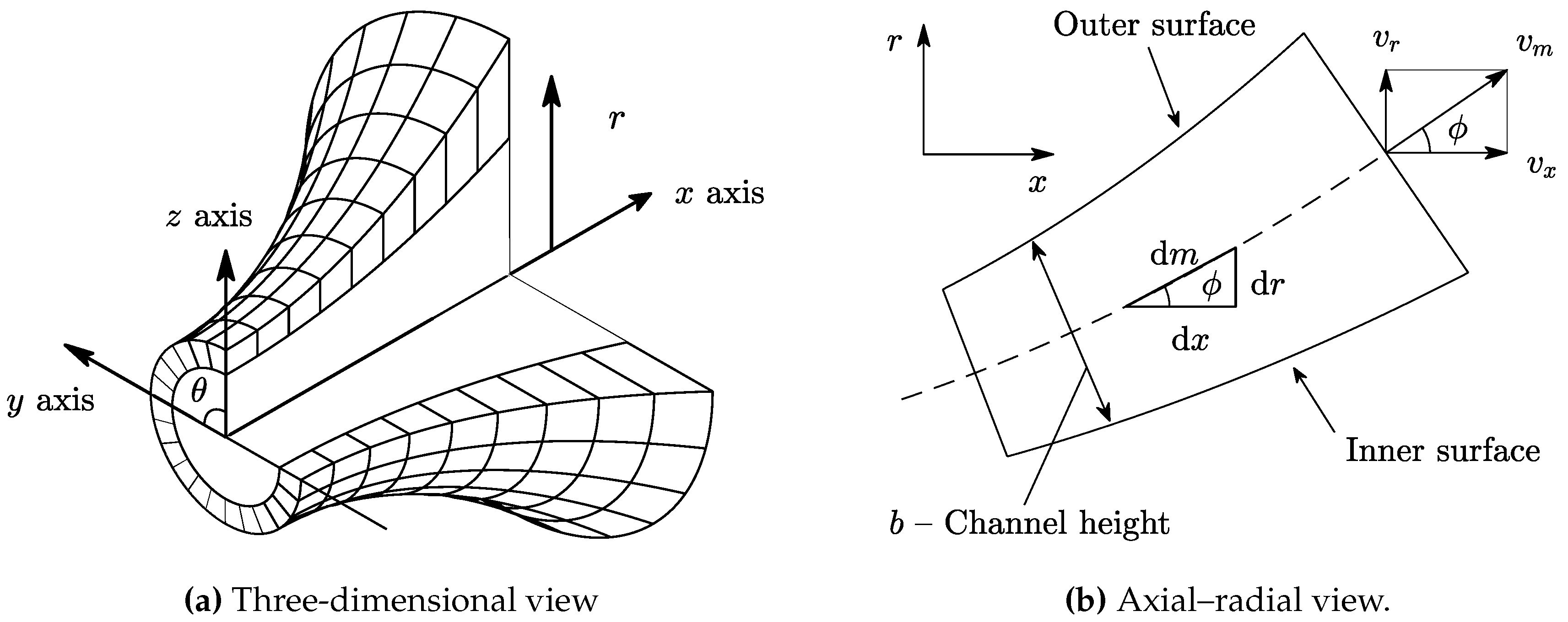
A sectioned view of a general annular diffuser geometry is shown in Figure 1a. The kinetic energy decreases and the static pressure increases as the fluid flows within the annular duct defined by the inner and outer surfaces. For the case of subsonic diffusers, the meridional component of velocity decreases when the flow area increases and the tangential component of velocity decreases when the mean radius of the channel increases [1].

In general, the meridional direction m will not be exactly aligned with the axial x or the radial r directions. This is illustrated in Figure 1b, where an axial–radial view of the diffuser is presented. The mean line of the diffuser can be parametrized as $r=r\left(m\right)$ and $x=x\left(m\right)$ such that the meridional, radial, and axial directions are related by the angle $\varphi$ given by Equation (3).

$$tan\varphi =\frac{\mathrm{d}r}{\mathrm{d}x}=\left(\frac{\mathrm{d}r}{\mathrm{d}m}\right)·{\left(\frac{\mathrm{d}x}{\mathrm{d}m}\right)}^{-1}$$

(3)

With this geometry the flow area is given by Equation (4), where r is the mean radius of the annular channel and b is height of the channel, measured normal to the meridional direction. The channel height can be prescribed as an arbitrary function of the meridional direction $b=b\left(m\right)$. The area ratio is defined as the ratio of outlet to inlet areas and is given by Equation (5).

$$\begin{array}{c}A=2\pi rb\end{array}$$

(4)

$$\begin{array}{c}AR=\frac{A_{\mathrm{out}}}{A_{\mathrm{in}}}\end{array}$$

(5)

This section described the geometry of a general annular diffuser. The particular geometry of straight wall annular diffusers is described under the heading geometry model.

2.2. Velocity Vector

In this work, the velocity is denoted by the symbol v, and the components are denoted by the subscripts $\theta$—tangential, m—meridional, x—axial, and r—radial. The velocity vector is illustrated in Figure 2 and the different components are given by Equations (6)–(9). The angle $\alpha$ is measured from the meridional towards the tangential direction.

$$\begin{array}{c}{v}_m=vcos\left(\alpha \right)\end{array}$$

(6)

$$\begin{array}{c}{v}_{\theta }=vsin\left(\alpha \right)\end{array}$$

(7)

$$\begin{array}{c}{v}_x=v_{m}cos\left(\varphi \right)=vcos\left(\varphi \right)cos\left(\alpha \right)\end{array}$$

(8)

$$\begin{array}{c}{v}_r=v_{m}sin\left(\varphi \right)=vsin\left(\varphi \right)cos\left(\alpha \right)\end{array}$$

(9)

2.3. Equations of State

The diffuser model was formulated in a general way and the thermodynamic properties of the working fluid can be computed with any set of equations of state that support pressure–density function calls. In this work, the REFPROP fluid library [26] was used for the computation of thermodynamic properties. The partial derivatives of fluid properties were computed using finite differences.

2.4. Mathematical Model

The diffuser model presented in this work is based on the transport equations for mass, meridional and tangential momentum, and energy in an annular channel. It assumes that the flow is one-dimensional (in the meridional direction), steady (no time variation), and axisymmetric (no circumferential variation). The model can use arbitrary equations of state and it accounts for effects of area change, heat transfer, and friction. Under these conditions the governing equations of the flow are given by Equations (10)–(13). These equations can be derived considering the mass, momentum, and energy balances for the infinitesimal control volume shown in Figure 3. The detailed derivation of these equations and a discussion of the physical meaning of the different terms is presented in the Appendix A.

$$\begin{array}{c}{v}_m\frac{\mathrm{d}\rho }{\mathrm{d}m}+\rho \frac{\mathrm{d}{v}_m}{\mathrm{d}m}=-\frac{\rho v_m}{br}\frac{\mathrm{d}}{\mathrm{d}m}\left(br\right)\end{array}$$

(10)

$$\begin{array}{c}\rho v_m\frac{\mathrm{d}{v}_m}{\mathrm{d}m}+\frac{\mathrm{d}p}{\mathrm{d}m}=\frac{\rho v_{\theta }^2}{r}sin\left(\varphi \right)-\frac{2{\tau }_{\mathrm{w}}}{b}cos\left(\alpha \right)\end{array}$$

(11)

$$\begin{array}{c}\rho v_m\frac{\mathrm{d}{v}_{\theta }}{\mathrm{d}m}=-\frac{\rho v_{\theta }{v}_m}{r}sin\left(\varphi \right)-\frac{2{\tau }_{\mathrm{w}}}{b}sin\left(\alpha \right)\end{array}$$

(12)

$$\begin{array}{c}\rho v_m\frac{\mathrm{d}p}{\mathrm{d}m}-\rho v_m{a}^2\frac{\mathrm{d}\rho }{\mathrm{d}m}=\frac{2({\tau }_{\mathrm{w}}v+{\dot{q}}_{\mathrm{w}})}{b{\left(\frac{\partial e}{\partial p}\right)}_{\rho }}\end{array}$$

(13)

Equations (10)–(13) pose a system of ordinary differential equations (ODE) that can be expressed more compactly in matrix form as given by Equation (14). The solution vector U, coefficient matrix A, and source term vector S are given by Equation (15).

$$\begin{array}{c}A\frac{\mathrm{d}U}{\mathrm{d}m}=S\end{array}$$

(14)

$$\begin{array}{c}A=\left[\begin{array}{cccc}\rho & 0& v_m& 0\\ \rho v_m& 0& 0& 1\\ 0& \rho v_m& 0& 0\\ 0& 0& -\rho v_m{a}^2& \rho v_m\end{array}\right]U=\left[\begin{array}{c}{v}_m\\ v_{\theta }\\ \rho \\ p\end{array}\right]S=\left[\begin{array}{c}-\frac{\rho v_m}{br}\frac{\mathrm{d}}{\mathrm{d}m}\left(br\right)\\ \frac{\rho v_{\theta }^2}{r}sin\left(\varphi \right)-\frac{2{\tau }_{\mathrm{w}}}{b}cos\left(\alpha \right)\\ -\frac{\rho v_{\theta }{v}_m}{r}sin\left(\varphi \right)-\frac{2{\tau }_{\mathrm{w}}}{b}sin\left(\alpha \right)\\ \frac{2({\tau }_{\mathrm{w}}v+{\dot{q}}_{\mathrm{w}})}{b{\left(\frac{\partial e}{\partial p}\right)}_{\rho }}\end{array}\right]\end{array}$$

(15)

It can be readily shown that the determinant of matrix A is given by Equation (16). This means that if the Mach number in the meridional direction is different than one, the matrix A can be inverted to compute the vector of derivatives $\frac{\mathrm{d}U}{\mathrm{d}m}$ according to Equation (17). In practice, matrix A is not inverted, instead the linear system of equations given by Equation (14) is solved using Gaussian elimination. It can be shown that the condition ${\mathrm{Ma}}_m=1$ corresponds to a choked diffuser. This means that the diffuser can only be choked due to the meridional component of velocity and that the tangential component of velocity can be decelerated from supersonic to subsonic velocities without shock waves [21].

$$\begin{array}{c}\det \left(A\right)={\rho }^3{v}_m^2{a}^2\left(\frac{v_m^2}{a^2}-1\right)={\rho }^3{v}_m^2{a}^2\left({\mathrm{Ma}}_m^2-1\right)\end{array}$$

(16)

$$\begin{array}{c}\frac{\mathrm{d}U}{\mathrm{d}m}=A^{-1}S\end{array}$$

(17)

The vector $\frac{\mathrm{d}U}{\mathrm{d}m}$ can be computed in this way for any integration step and then used as input for an explicit numerical method to solve ordinary differential equations. The integration starts from the initial values (see Section 2.5) and stops when the prescribed value of the outlet to inlet area ratio $AR$ is reached. In this work, the MATLAB function ode45 [27] was used to perform the numerical integration. This function uses an automatic-stepsize-control solver that combines fourth and fifth order Runge–Kutta methods.

To compute the source term vector, it is necessary to prescribe the geometry of the diffuser, i.e., the variation of the channel height $b\left(m\right)$ and radius $r\left(m\right)$ in the meridional direction, and to provide models for the shear stress ${\tau }_{\mathrm{w}}$ and the heat flux ${\dot{q}}_{\mathrm{w}}$ at the walls.

2.4.1. Geometry Sub-Model

The diffuser model was formulated in a general way such that the geometry can be described by any set of arbitrary functions $r=r\left(m\right)$, $x=x\left(m\right)$, and $b=b\left(m\right)$. Although the one-dimensional model presented in this work can accept any geometry as input, it is not able to predict flow features such as boundary layer separation. For this reason, this type of simplified model is not well suited for a detailed geometry design of the diffuser.

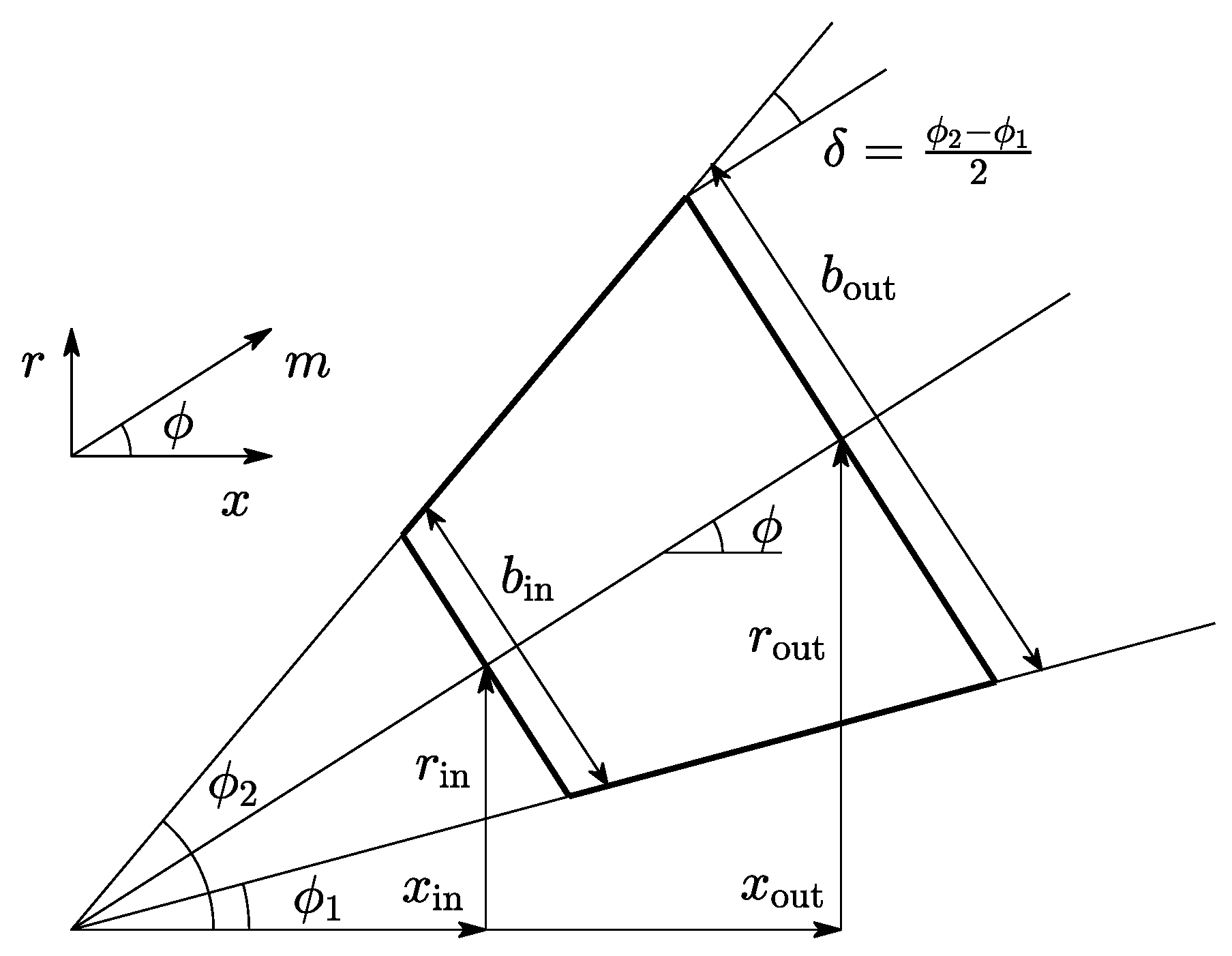
Despite this, one-dimensional models can give a good indication of the expected performance of a well-designed diffuser (in terms of the pressure recovery coefficient). For this reason, the main purpose of the diffuser model presented in this paper is to serve as a realistic boundary condition at the outlet of turbomachinery that reacts to changes in the design variables during the preliminary design and optimization. In addition, the diffuser geometry obtained from this type of analysis can be used as the starting point for a more detailed diffuser design such as a CFD-based shape optimization. Within this context, the geometry of the diffuser was modeled in a simple way assuming that the inner and outer surfaces are straight. These types of diffusers are known as conical wall annular diffusers (also as straight wall annular diffusers) and their geometry is shown in Figure 4.

For this particular geometry, the angle $\varphi$ is constant and it is given as the arithmetic mean of the inner and outer wall cant angles, $\varphi =({\varphi }_1+{\varphi }_2)/2$. The relations $r=r\left(m\right)$, $x=x\left(m\right)$, and $b=b\left(m\right)$ can be deduced from Figure 4 and they are given by Equations (18)–(20), where $\delta =({\varphi }_2-{\varphi }_1)/2$ is the divergence semi-angle.

$$\begin{array}{c}r\left(m\right)=r_{\mathrm{in}}+msin\left(\varphi \right)\end{array}$$

(18)

$$\begin{array}{c}x\left(m\right)=x_{\mathrm{in}}+mcos\left(\varphi \right)\end{array}$$

(19)

$$\begin{array}{c}b\left(m\right)=b_{\mathrm{in}}+2mtan\left(\delta \right)\end{array}$$

(20)

2.4.2. Friction Sub-Model

The friction is modeled as a body force that does not do work (this models the no-slip condition at the walls). This is the approach often used in one-dimensional flow models because they cannot take into account the velocity gradient in the direction normal to the wall [21,24].

The viscous stress at the wall ${\tau }_{\mathrm{w}}$ is computed in terms of the skin friction coefficient $C_{\mathrm{f}}$ as given by Equation (21). The viscous force is assumed to have the opposite direction as the velocity vector such that the friction components in the meridional and tangential direction are given by $-{\tau }_{\mathrm{w}}cos\left(\alpha \right)$ and $-{\tau }_{\mathrm{w}}sin\left(\alpha \right)$, respectively, see Figure 3.

$${\tau }_{\mathrm{w}}=C_{\mathrm{f}}\frac{\rho v^2}{2}$$

(21)

To the knowledge of the authors there are no available correlations to predict the skin friction coefficient in annular channels with swirling flow. Using ordinary skin friction correlations for internal flows is discouraged because they do not consider the influence of swirl on the shear stress at the wall.

However, it is possible to estimate a reasonable value for the skin friction coefficient based on experimental data from existing vaneless diffusers. Brown [28] measured the local skin friction coefficient for different vaneless diffusers and obtained values in the range 0.003–0.010. In the absence of better estimates, Johnston–Dean [22] recommend values within the range 0.005–0.010 for the global skin friction coefficient. In a similar way, Dubitsky–Japikse [24] suggest 0.010 as a reasonable estimate for the global skin friction coefficient, but noted that values from 0.005 to 0.020 were required to fit experimental data, depending on the application. The values that were reported in this paragraph are meaningful for well-designed diffusers without flow separation.

2.4.3. Heat Transfer Sub-Model

The universal approach in the design and analysis of diffusers for turbomachinery applications is to neglect heat transfer and assume that the flow is adiabatic ${\dot{q}}_{\mathrm{w}}=0$. To the knowledge of the authors, Stanitz [21] is the only reference that accounts for the effect of heat transfer in the energy transport equation. Although heat transfer is usually neglected, the heat transfer modeling is discussed in this section for the sake of completeness.

Stanitz [21] suggests that the heat flux is proportional to the temperature difference between the fluid and the wall as given by Equation (22), where the wall temperature is prescribed as a function of the meridional direction $T_{\mathrm{w}}\left(m\right)$. This equation uses the stagnation temperature of the fluid instead of the static temperature because the fluid is at rest at the wall (a recovery factor of unity is assumed).

$${\dot{q}}_{\mathrm{w}}=U(T_{\mathrm{w}}-T_0)$$

(22)

In addition, Stanitz [21] suggests to use the Reynolds analogy given by Equations (23) and (24), to obtain an approximate value for the heat transfer coefficient in terms of the skin friction coefficient, where the usual definitions for the Nusselt number $\mathrm{Nu}=\frac{U{D}_{\mathrm{h}}}{k}$, Reynolds number $\mathrm{Re}=\frac{\rho v{D}_{\mathrm{h}}}{k}$, and Prandtl number $\mathrm{Pr}=\frac{c_p\mu }{k}$ are used. The hydraulic diameter of an annular duct is given by the channel height ($D_{\mathrm{h}}=b$), but it is immaterial for the computation of the heat transfer coefficient.

$$\begin{array}{c}\mathrm{Nu}=\frac{1}{2}{C}_{\mathrm{f}}\mathrm{Re}\mathrm{Pr}\end{array}$$

(23)

$$\begin{array}{c}U=\frac{\rho v{c}_p}{2}{C}_{\mathrm{f}}\end{array}$$

(24)

It is also possible to use the Chilton–Colburn analogy [29] (pp. 358–360) given by Equations (25) and (26) to estimate the heat transfer coefficient. This analogy extends the Reynolds analogy to fluids with a Prandtl number different from one.

$$\begin{array}{c}\mathrm{Nu}=\frac{1}{2}{C}_{\mathrm{f}}\mathrm{Re}{\mathrm{Pr}}^{1/3}\end{array}$$

(25)

$$\begin{array}{c}U=\frac{\rho v{c}_p}{2}{C}_{\mathrm{f}}{\mathrm{Pr}}^{-2/3}\end{array}$$

(26)

Both these analogies can be used to get a rough estimate of the heat transfer coefficient from a known value of the skin friction coefficient. Using ordinary heat transfer correlations for internal flows is discouraged, because they do not take into account the impact of the swirl into the heat transfer process.

2.5. Connection with a Turbomachinery Model

This section describes the link between the diffuser model presented in this work and a generic turbomachinery model. The initial conditions for the integration of the diffuser model are given by Equation (27), where it is assumed that the thermodynamic state and velocity vector do not change from the turbomachine outlet to the diffuser inlet.

$$U^0={\left[\begin{array}{c}{v}_m\\ v_{\theta }\\ \rho \\ p\end{array}\right]}^0={\left[\begin{array}{c}{v}_m\\ v_{\theta }\\ \rho \\ p\end{array}\right]}^{\mathrm{out}}$$

(27)

To describe the geometry of the diffuser, the mean radius $r_{\mathrm{in}}$ and the channel height $b_{\mathrm{in}}$ at the inlet are obtained from the turbomachine outlet radius $R_{\mathrm{out}}$ and blade height $H_{\mathrm{out}}$ as given by Equations (28) and (29), see Figure 5.

$$\begin{array}{c}{r}_{\mathrm{in}}=R_{\mathrm{out}}\end{array}$$

(28)

$$\begin{array}{c}{b}_{\mathrm{in}}=H_{\mathrm{out}}/cos\left(\varphi \right)\end{array}$$

(29)

In addition, it is necessary to prescribe the area ratio $AR$ as the termination criterion for the integration of the ODE system and the inner ${\varphi }_1$ and outer ${\varphi }_2$ wall angles. Equivalently, it is possible to prescribe the mean cant angle $\varphi =({\varphi }_1+{\varphi }_2)/2$ and the divergence semi-angle $\delta =({\varphi }_2-{\varphi }_1)/2$. These geometric parameters can be specified as fixed parameters or independent variables during the preliminary design and optimization of a turbomachine.

3. Verification and Validation of the Model

The aim of this section is the verification (solving the equations right) and validation (solving the right equations) of the diffuser model and solution algorithm proposed in this work. To verify the model, the reference case summarized in

Table 3. Definition of the reference case.

Variable	Symbol	Value
Working fluid	-	Air
Inlet static pressure	$p_{\mathrm{in}}$	101.3 kPa
Inlet static temperature	$T_{\mathrm{in}}$	20.0 ${}^{\circ }$C
Inlet meridional Mach	${\mathrm{Ma}}_{\mathrm{m},\mathrm{in}}$	0.30
Inlet swirl angle	${\alpha }_{\mathrm{in}}$	30.0${}^{\circ }$
Turbomachine outlet radius	$R_{\mathrm{out}}$	1.0 m
Outlet hub-to-tip ratio	${(r_{\mathrm{h}}/r_{\mathrm{t}})}_{\mathrm{out}}$	0.7
Mean wall cant angle	$\varphi$	30.0${}^{\circ }$
Divergence semi-angle	$\delta$	5.0${}^{\circ }$
Diffuser area ratio	$AR$	1.0–5.0
Skin friction coefficient	$C_{\mathrm{f}}$	0.010
Heat transfer coefficient	U	0 W/m${}^2·$K

was analyzed and the error of the numerical solution in terms of stagnation enthalpy and entropy was assessed. The case study proposed considers a subsonic flow of air within the annular diffuser at the outlet of an axial turbine or compressor. The skin friction coefficient was assumed to be $C_{\mathrm{f}}=0.010$ based on the suggestions from [22,24,28] and the heat transfer was neglected.

In the absence of heat transfer, the stagnation enthalpy of the flow remains constant, see the Appendix A, and any change in stagnation enthalpy is due to numerical error. The relative stagnation enthalpy error was evaluated using Equations (30) and (31) and it is shown as a function of the diffuser area ratio in Figure 6. It can be seen that the stagnation enthalpy is properly conserved and the relative error is of the order of 10${}^{-9}$, which is smaller than the prescribed relative tolerance of 10${}^{-6}$ for the integration of the ODE system.

$$\begin{array}{c}{h}_{0,\mathrm{error}}=\frac{|h_0-h_{0,\mathrm{in}}|}{h_{0,\mathrm{in}}}\end{array}$$

(30)

$$\begin{array}{c}{h}_0=h(p,\rho )+\frac{v_m^2}{2}+\frac{v_{\theta }^2}{2}\end{array}$$

(31)

In a similar way, the entropy error was analyzed. The entropy of the flow was computed using pressure–density function calls to the equation of state (EoS) at each integration step, Equation (32), and also evaluated integrating the transport equation for entropy given by Equation (33), where $\dot{\sigma }$ is the rate of entropy generation per unit volume due to friction. See the Appendix A for the details about the derivation of the transport equation for entropy. The entropy error was evaluated using Equation (34) and it is shown as a function of the diffuser area ratio in Figure 6. It can be observed that the relative entropy error is of the order of 10${}^{-7}$, which is smaller than the prescribed integration tolerance of 10${}^{-6}$. As both the stagnation enthalpy and entropy errors are smaller than the prescribed tolerance, we can conclude that the solution algorithm solves the flow equations satisfactorily.

$$\begin{array}{c}{s}_{\mathrm{EoS}}=s(p,\rho )\end{array}$$

(32)

$$\begin{array}{c}\rho v_m\left(\frac{\mathrm{d}{s}_{\mathrm{gen}}}{\mathrm{d}m}\right)=\dot{\sigma }=2\frac{{\tau }_{\mathrm{w}}v}{bT}\end{array}$$

(33)

$$\begin{array}{c}{s}_{\mathrm{error}}=\frac{|s_{\mathrm{EoS}}-s_{\mathrm{gen}}|}{s_{\mathrm{EoS}}}\end{array}$$

(34)

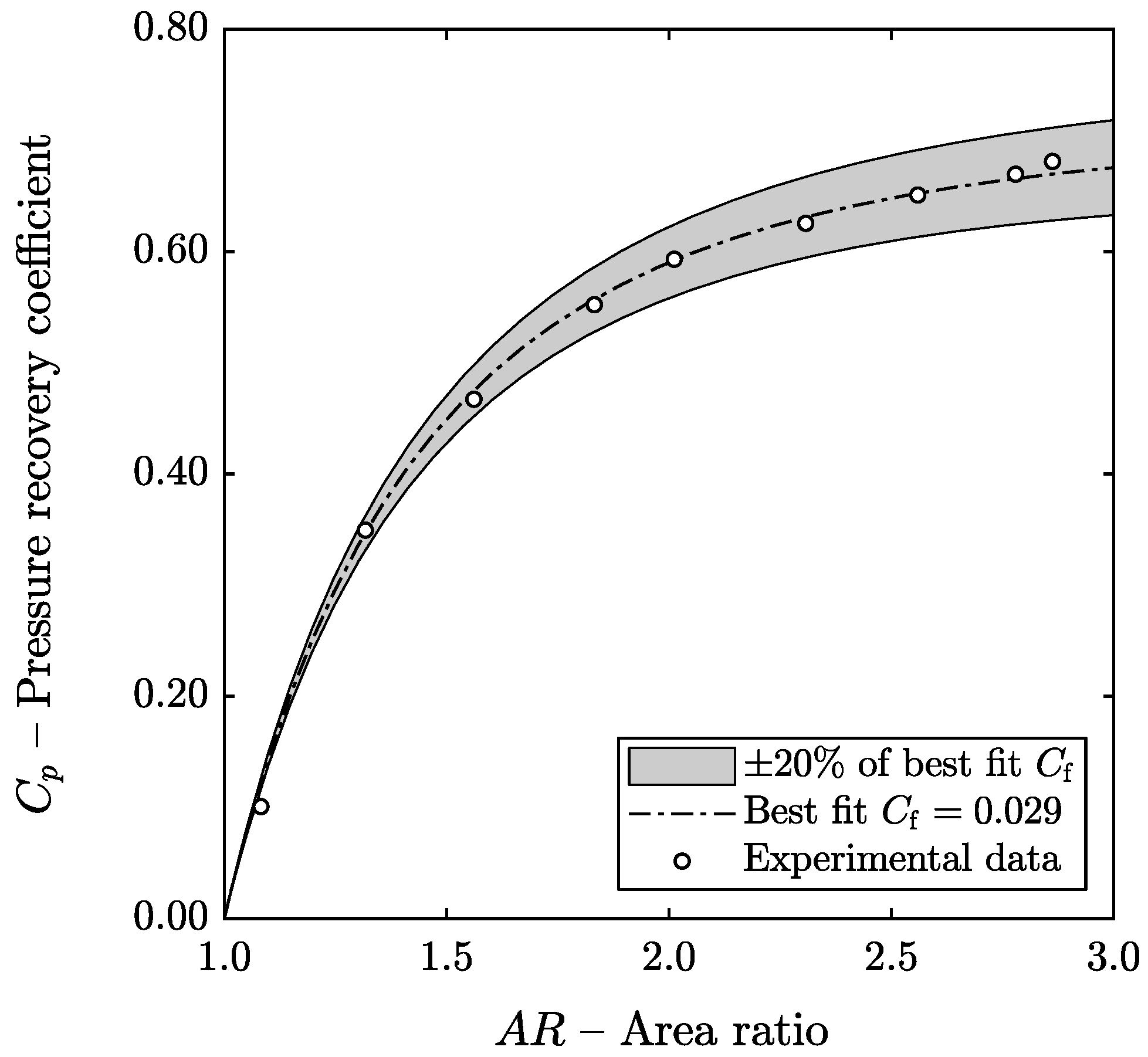
In addition, the diffuser model was validated against the annular diffuser experimental data from Kumar and Kumar [30]. The conditions that define this case are summarized in

Table 4. Definition of the validation case from Kumar and Kumar [30].

Variable	Symbol	Value
Working fluid	-	Air
Inlet static pressure	$p_{\mathrm{in}}$	101.3 kPa
Inlet static temperature	$T_{\mathrm{in}}$	20.0 ${}^{\circ }$C
Inlet meridional Mach	${\mathrm{Ma}}_{\mathrm{m},\mathrm{in}}$	0.07
Inlet swirl angle	${\alpha }_{\mathrm{in}}$	0.0${}^{\circ }$
Inlet mean radius	$r_{\mathrm{in}}$	57.8 mm
Inlet channel height	$b_{\mathrm{in}}$	39.5 mm
Mean wall cant angle	$\varphi$	${15.0}^{\circ }$
Divergence semi-angle	$\delta$	0.0${}^{\circ }$
Diffuser area ratio	$AR$	1.0–3.0
Skin friction coefficient	$C_{\mathrm{f}}$	Fitted to data
Heat transfer coefficient	U	0 W/m${}^2·$K

and the experimental and computed pressure recovery coefficients are compared in

Table 5. Comparison of the model output with the experimental data from Kumar and Kumar [30].

$\mathbf{AR}$	${\mathit{C}}_{\mathit{p}}^{\mathbf{exp}}$	${\mathit{C}}_{\mathit{p}}^{\mathbf{model}}$	Relative Error
1.082	0.101	0.122	21.27%
1.317	0.349	0.347	−0.64%
1.561	0.467	0.475	1.73%
1.832	0.552	0.557	0.89%
2.012	0.593	0.592	−0.14%
2.308	0.626	0.631	0.89%
2.560	0.651	0.653	0.23%
2.779	0.670	0.666	−0.58%
2.863	0.681	0.670	−1.67%

and in Figure 7. The heat transfer was neglected for the validation ($U=0$) because the experimental data from Kumar and Kumar [30] corresponds to a low-speed annular diffuser where the difference between fluid temperature and wall temperature is expected to be very small. The skin friction coefficient was fitted to minimize the two-norm of the error between the experimental data and the model output. In addition, the range of variation of the pressure recovery coefficient for skin friction coefficients ranging between $\pm 20\%$ of the best-fit value is shown as a shaded area to illustrate the impact of this parameter on the diffuser performance.

Ignoring the point corresponding to $AR=1.082$, it can be observed that the relative deviation of the pressure recovery coefficient is always less than 2% when the best-fit skin friction coefficient ($C_{\mathrm{f}}=0.029$) is used. It is plausible that the deviation between experiment and model when $AR=1.082$ is due to the development of the flow at the inlet of the diffuser. This analysis shows that the model can be used to make accurate predictions when skin friction coefficient can be fitted to experimental data or approximate predictions in cases where there is no experimental data available.

4. Sensitivity Analysis

This section contains a sensitivity analysis of the reference case from Table 3 to gain insight about the impact of several input parameters on diffuser performance. The next sections investigate the influence of: (1) skin friction coefficient, (2) inlet hub-to-tip ratio, (3) mean wall cant angle, (4) inlet swirl angle, and (5) inlet meridional Mach number on the pressure recovery coefficient as a function of diffuser area ratio. The divergence semi-angle was not included in the analysis because increasing this parameter may lead to boundary layer separation close to the walls and the model used in this work cannot predict this phenomenon (Kline et al. [31] provide stability maps that can be used to predict flow separation for straight-walled and conical diffusers as a function of divergence semi-angle and area ratio. However, the authors are not aware of similar maps for annular diffusers in the open literature). Each of the analyses studies the influence of one variable while the other parameters are the same as in the reference case (one-at-a-time sensitivity analysis) and the ranges of the variables were selected to cover the flow conditions typical of most turbomachinery applications.

In addition, the influence of heat transfer on diffuser performance was analyzed for different wall temperatures using the Chilton–Colburn analogy to estimate the heat transfer coefficient. As expected, heat addition accelerates the flow and penalizes the pressure recovery coefficient. The details of the heat transfer investigations are not reported because the influence of heat addition was secondary compared to that of the other input parameters.

4.1. Influence of the Skin Friction Coefficient

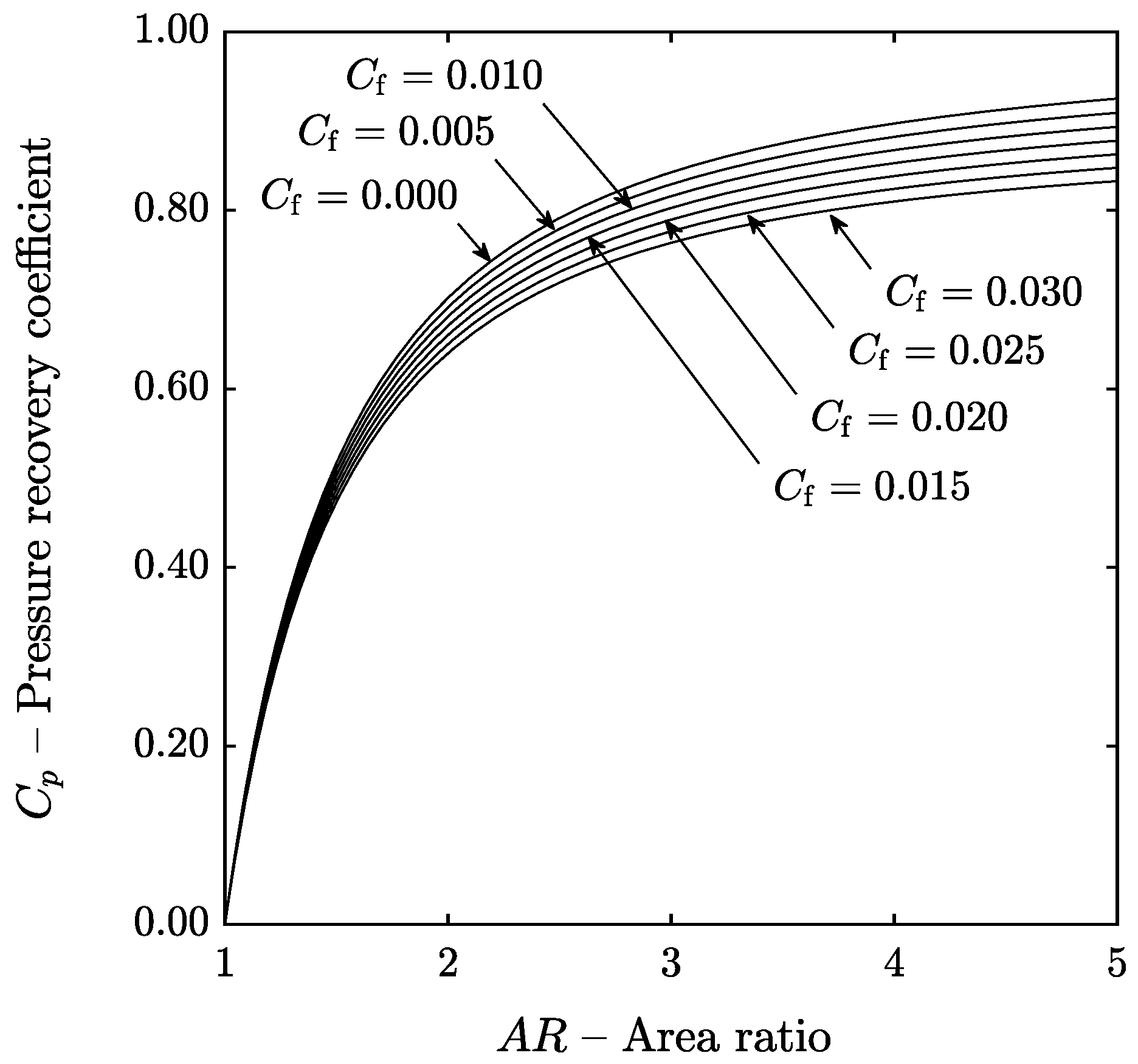
As discussed in Section 2, to the knowledge of the authors, there are no correlations available to predict the skin friction coefficient in annular channels with swirling flow, but it is possible to estimate a realistic value based on the existing literature. The friction factor was varied from 0.000 (frictionless) to 0.030 (high friction) and the impact on the pressure recovery coefficient as a function of the area ratio is shown in Figure 8.

It can be observed that increasing the friction factor decreases the pressure recovery in a linear way (the different curves are equispaced) and that the effect is more notable when the area ratio increases (since the length of the channel increases). For the reference case considered, the pressure recovery increases with the area ratio in a monotonous manner and has an asymptotic behavior, irrespective of the numerical value of the friction coefficient. This suggest that an optimum value of the area ratio that maximizes the pressure recovery does not exist and that the pressure recovery always increases with the area ratio up to a limiting value.

This, perhaps counter-intuitive, result may be explained as the consequence of two conflicting effects. On the one hand, when the area ratio increases the diffuser length and wetted surface increase. However, as the area ratio increases the velocity and shear stress at the wall are reduced (the shear stress is proportional to the dynamic pressure). If this second effect dominates, friction becomes negligible and the pressure recovery increases asymptotically as the area ratio tends to infinity.

4.2. Influence of the Inlet Hub-to-Tip Ratio

To accommodate the density change, the hub-to-tip ratio is usually high at the outlet of axial compressors and low at the outlet of axial turbines. In this section, the hub-to-tip ratio at the inlet of the diffuser was varied between 0.50 and 0.95 and the results were plotted in Figure 9. It can be observed that the diffuser performance is penalized as the hub-to-tip ratio increases and that the effect is not linear: the pressure recovery coefficient is reduced more rapidly at high hub-to-tip ratios.

The reason for this behavior is that when the hub-to-tip ratio increases, the channel height of the diffuser is reduced according to Equation (35) and, since the channel height appears in the denominator of the friction terms of the momentum equations, Equations (11) and (12), the diffuser performance declines. Another interpretation based on physical intuition is that the channel height is the hydraulic diameter of the annular diffuser and that reducing this parameter will increase the friction losses.

$$b_{\mathrm{in}}=H_{\mathrm{out}}/cos\left(\varphi \right)=2R_{\mathrm{out}}{\left(\frac{1-(r_{\mathrm{h}}/r_{\mathrm{t}})}{1+(r_{\mathrm{h}}/r_{\mathrm{t}})}\right)}_{\mathrm{out}}/cos\left(\varphi \right)$$

(35)

4.3. Influence of the Mean Wall Cant Angle

Figure 10a shows the pressure recovery coefficient as a function of the area ratio when the mean cant angle is varied from 0${}^{\circ }$ to 40${}^{\circ }$. It can be seen that the pressure recovery coefficient is very low when $\varphi =0^{\circ }$ because the radius of the diffuser remains constant and the tangential component of velocity is not recovered and that it increases very quickly as the mean cant angle increases (for instance from 0${}^{\circ }$ to 10${}^{\circ }$). Further increasing the mean wall cant angle will only improve the pressure recovery marginally (the change from 30${}^{\circ }$ to 40${}^{\circ }$ is almost inappreciable).

The same results are plotted as a function of the normalized axial length (instead of the area ratio) in Figure 10b. The end of the lines corresponds to the point where $AR=5$. It can be observed that for a fixed diffuser axial length, the pressure recovery coefficient increases as the mean wall cant angle increases because both the area and the mean radius of the channel increase.

These results illustrate that the mean cant angle is not a critical parameter when there are no space limitations, but that adopting a high mean wall cant angle is advantageous when the maximum axial length of the diffuser is constrained.

4.4. Influence of the Inlet Swirl Angle

In this section, the influence of the inlet swirl angle for a fixed meridional velocity was investigated. The results from Figure 11 show that increasing the inlet swirl angle decreases the pressure recovery coefficient of the diffuser and that this effect is more marked at higher swirl angles. The reason for this is that the presence of swirl increases the available dynamic pressure at the inlet and, for this reason, the area ratio required to reach the same pressure recovery coefficient as for the case $\alpha =0^{\circ }$ is higher. Moreover, the presence of swirl leads to wall shear stress in the circumferential direction that increases the friction losses.

4.5. Influence of the Inlet Mach Number

The influence of the inlet Mach number (compressibility effects) on the diffuser performance, including the limiting case of incompressible flow, is shown in Figure 12. The analysis presented on this section was performed assuming frictionless flow instead of $C_{\mathrm{f}}=0.010$ in order to compare the results at different inlet Mach numbers with the analytical results for inviscid, incompressible flow given by Equation (36). This equation is a well-known result [1,22] that can be proved integrating the mass and momentum equations, Equations (10)–(12), for constant density and zero wall shear stress.

It can be observed that the model predicts a modest increase on the pressure recovery coefficient as the inlet Mach number increases. In addition, the results obtained when the inlet meridional Mach number is 0.30 or lower (low-speed flow) are consistent with the analytical results for incompressible flow. This result can be regarded as part of the model verification.

$$C_{p,\mathrm{incompressible}}=1-\frac{tan{\left({\alpha }_{\mathrm{in}}\right)}^2+{\left(\frac{b_{\mathrm{in}}}{b}\right)}^2}{1+tan{\left({\alpha }_{\mathrm{in}}\right)}^2}·{\left(\frac{r_{\mathrm{in}}}{r}\right)}^2$$

(36)

5. Conclusions

A one-dimensional flow model for annular diffusers was proposed and the connection of this model with the preliminary design and optimization of turbomachinery was discussed. The model formulation is more general than that of previous literature as it is possible to use arbitrary equations of state and include the effects of area change, heat transfer, and friction. The mathematical model poses a system of ordinary differential equations and it was shown that: (1) the solution is undetermined when the Mach number in the meridional direction is one (the flow is choked) and (2) the Mach number in the circumferential direction does not compromise the solution. In addition, the detailed derivation of the equations (omitted in other works) was presented in the Appendix A to provide physical insight about the flow in annular channels.

The model was verified against a reference case assessing that: (1) the stagnation enthalpy is conserved, (2) the entropy generation computed using the equation of state and using the second law of thermodynamics is consistent and it was found that the error of the numerical solution was always smaller than the prescribed integration tolerance. In addition, the model was validated against the experimental data from Kumar and Kumar [30], finding that the relative deviation between the predicted and measured pressure recovery coefficients was always less than 2% when the best-fit skin friction coefficient is used.

A sensitivity analysis was performed to investigate the influence of the: (1) skin friction coefficient, (2) inlet hub-to-tip ratio, (3) mean wall cant angle, (4) inlet swirl angle, and (5) inlet meridional Mach number on the diffuser performance. The ranges of these variables were selected to cover the flow conditions typical of most turbomachinery applications. The following conclusions were gathered:

• The pressure recovery coefficient increases asymptotically as the area ratio tends to infinity, regardless of the value of the skin friction coefficient. This suggest that the area ratio is not a suitable optimization variable during the diffuser design when the size of the diffuser is not constrained.
• The inlet hub-to-tip ratio has a strong impact on the pressure recovery because it is closely related to the channel height of the diffuser. The pressure recovery is penalized when the hub-to-tip ratio increases, and the trend is nonlinear: the pressure recovery coefficient is reduced more rapidly at high hub-to-tip ratios. This implies that in general, the design of efficient diffusers for axial compressors (high hub-to-tip ratios and short blades at the last stage) is more challenging than that of axial turbines (low hub-to-tip ratios and long blades at the last stage).
• The pressure recovery is very low when the mean wall cant angle is zero because the radius of the diffuser remains constant and the tangential component of velocity is not recovered. This shows that the diffuser should be designed with an increasing mean radius to recover the kinetic energy of swirling flows effectively.
• Assuming that there is no flow separation, increasing the mean wall cant angle always improves the pressure recovery. However, for a given area ratio the mean wall cant angle has only a small impact on the pressure recovery, while for a given axial length increasing the mean wall cant angle improves the pressure recovery significantly. This implies that the mean wall cant angle is not a critical parameter when there are no space limitations, but that adopting a high mean wall cant angle is advantageous when the maximum axial length of the diffuser is constrained.
• Increasing the swirl angle at the inlet of the diffuser reduces the pressure recovery coefficient because the wall shear stress in the circumferential direction is increased. This implies that the diffuser performance will be improved if the velocity triangle of the last turbomachinery stage is designed so that the absolute velocity has a small tangential component.
• The pressure recovery coefficient increases as the inlet meridional Mach number increases. The effect on the inlet Mach number has only a modest impact on the pressure recovery, compared with the other variables. In addition, it was found that when the inlet meridional Mach number is lower than 0.30 the results from the compressible and incompressible analyses are almost identical.

References

- Lohmann, R.; Markowski, S.; Brookman, E. Swirling Flow Through Annular Diffusers with Conical Walls. J. Fluids Eng. 1979, 101, 224–229. [Google Scholar] [CrossRef]
- White, F.M. Fluid Mechanics, 7th ed.; McGraw-Hill: New York, NY, USA, 2011. [Google Scholar]
- Macchi, E.; Perdichizzi, A. Efficiency Prediction for Axial-Flow Turbines Operating with Nonconventional Fluids. J. Eng. Power 1981, 103, 718–724. [Google Scholar] [CrossRef]
- Bahamonde, S.; Pini, M.; De Servi, C.; Rubino, A.; Colonna, P. Method for the Preliminary Fluid Dynamic Design of High-Temperature Mini-Organic Rankine Cycle Turbines. J. Eng. Gas Turbines Power 2017, 139, 1–14. [Google Scholar] [CrossRef]
- Lozza, G.; Macchi, E.; Perdichizzi, A. On the Influence of the Number of Stages on the Efficiency of Axial-Flow Turbines. In Proceedings of the International Gas Turbine Conference and Exhibition, London, UK, 18–22 April 1982; pp. 1–10. [Google Scholar]
- Da Lio, L.; Manente, G.; Lazzaretto, A. New Efficiency Charts for the Optimum Design of Axial Flow Turbines for Organic Rankine Cycles. Energy 2014, 77, 447–459. [Google Scholar] [CrossRef]
- Astolfi, M.; Macchi, E. Efficiency Correlations for Axial Flow Turbines Working with Non-Conventional Fluids. In Proceedings of the 3rd International Seminar on ORC Power System, ASME-ORC2015, Brussels, Belgium, 12–14 October 2015; pp. 1–12. [Google Scholar]
- Da Lio, L.; Manente, G.; Lazzaretto, A. Predicting the Optimum Design of Single Stage Axial Expanders in ORC Systems: Is There a Single Efficiency Map for Different Working Fluids? Appl. Energy 2016, 167, 44–58. [Google Scholar] [CrossRef]
- Al Jubori, A.; Dadah, R.K.A.; Mahmoud, S.; Khalil, K.M.; Ennil, A.S.B. Development of Efficient Small Scale Axial Turbine for Solar Driven Organic Rankine Cycle. In Proceedings of the ASME Turbo Expo 2016, Seoul, Korea, 13–17 June 2016; pp. 1–11. [Google Scholar]
- Talluri, L.; Lombardi, G. Simulation and Design Tool for ORC Axial Turbine Stage. Energy Procedia 2017, 129, 277–284. [Google Scholar] [CrossRef]
- Tournier, J.M.; El-Genk, M.S. Axial Flow, Multi-Stage Turbine and Compressor Models. Energy Convers. Manag. 2010, 51, 16–29. [Google Scholar] [CrossRef]
- Meroni, A.; La Seta, A.; Andreasen, J.; Pierobon, L.; Persico, G.; Haglind, F. Combined Turbine and Cycle Optimization for Organic Rankine Cycle Power Systems–Part A: Turbine Model. Energies 2016, 9, 313. [Google Scholar] [CrossRef]
- Meroni, A.; La Seta, A.; Andreasen, J.; Pierobon, L.; Persico, G.; Haglind, F. Combined Turbine and Cycle Optimization for Organic Rankine Cycle Power Systems–Part B: Case Study. Energies 2016, 9, 393. [Google Scholar] [CrossRef]
- Meroni, A.; Graa, J.; Persico, G.; Haglind, F. Optimization of Organic Rankine Cycle Power Systems Considering Multistage Axial Turbine Design. Appl. Energy 2018, 209, 339–354. [Google Scholar] [CrossRef]
- Perdichizzi, A.; Lozza, G. Design Criteria and Efficiency Prediction for Radial Inflow Turbines. In Proceedings of the International Gas Turbine Conference and Exhibition, Anaheim, CA, USA, 31 May–4 June 1987; pp. 1–9. [Google Scholar]
- Uusitalo, A.; Turunen-saaresti, T.; Honkatukia, J.; Backman, J. Combined Thermodynamic and Turbine Design Analysis. In Proceedings of the 3rd International Seminar on ORC Power System, ASME-ORC2015, Brussels, Belgium, 12–14 October 2015; pp. 1–10. [Google Scholar]
- Rahbar, K.; Mahmoud, S.; Al-Dadah, R.K.; Moazami, N. Parametric Analysis and Optimization of a Small-Scale Radial Turbine for Organic Rankine Cycle. Energy 2015, 83, 696–711. [Google Scholar] [CrossRef]
- Da Lio, L.; Manente, G.; Lazzaretto, A. A Mean-Line Model to Predict the Design Efficiency of Radial Inflow Turbines in Organic Rankine Cycle (ORC) Systems. Appl. Energy 2017, 205, 187–209. [Google Scholar] [CrossRef]
- Pini, M.; Persico, G.; Casati, E.; Dossena, V. Preliminary Design of a Centrifugal Turbine for Organic Rankine Cycle Applications. J. Eng. Gas Turbines Power 2013, 135, 042312. [Google Scholar] [CrossRef]
- Casati, E.; Vitale, S.; Pini, M.; Persico, G.; Colonna, P. Centrifugal Turbines for Mini-ORC Power Systems. J. Eng. Gas Turbines Power 2014, 136, 11. [Google Scholar] [CrossRef]
- Stanitz, J.D. One-Dimensional Compressible Flow in Vaneless Diffusers of Radial- and Mixed-Flow Centrifugal Compressors, Including Effects of Friction, Heat Transfer and Area Change; National Advisory Committee for Aeronautics: Washington, DC, USA, 1952.
- Johnston, J.P.; Dean, R.C. Losses in Vaneless Diffusers of Centrifugal Compressors and Pumps: Analysis, Experiment, and Design. J. Eng. Power 1966, 88, 49–60. [Google Scholar] [CrossRef]
- Elgammal, A.; Elkersh, A. A Method for Predicting Annular Diffuser Performance with Swirling Inlet Flow. J. Mech. Eng. Sci. 1981, 23, 107–112. [Google Scholar] [CrossRef]
- Dubitsky, O.; Japikse, D. Vaneless Diffuser Advanced Model. J. Turbomach. 2008, 130, 1–10. [Google Scholar] [CrossRef]
- Agromayor, R.; Nord, L.O. AnnularDiffuser1D—A One-Dimensional Model for the Performance Prediction of Annular Diffusers. 2019. Available online: https://doi.org/10.5281/zenodo.2634095 (accessed on 13 September 2019).
- Lemmon, E.W.; Huber, M.L.; McLinden, M.O. NIST Standard Reference Database 23: Reference Fluid Thermodynamic and Transport Properties-REFPROP, Version 9.1; National Institute of Standards and Technology: Gaithersburg, MD, USA, 2013.
- Shampine, L.F.; Reichelt, M.W. The MATLAB ODE Suite. SIAM J. Sci. Comput. 1997, 18, 1–22. [Google Scholar] [CrossRef] [Green Version]
- Brown, W.B. Friction Coefficients in a Vaneless Diffuser; National Advisory Committee for Aeronautics: Washington, DC, USA, 1947.
- Cengel, Y.A. Heat Transfer: A Practical Approach, 2nd ed.; McGraw-Hill: New York, NY, USA, 2002. [Google Scholar]
- Kumar, D.S.; Kumar, K.L. Effect of Swirl on Pressure Recovery in Annular Diffusers. J. Mech. Eng. Sci. 1980, 22, 305–313. [Google Scholar] [CrossRef]
- Kline, S.J.; Abbott, D.E.; Fox, R.W. Optimum Design of Straight-Walled Diffusers. J. Basic Eng. 1959, 81, 321–329. [Google Scholar] [CrossRef]
- Aungier, R.H. Turbine Aerodynamics, 1st ed.; ASME Press: New York, NY, USA, 2006. [Google Scholar]
Figure 1.
Geometry of a general annular diffuser.
Figure 2.
Decomposition of the velocity vector.
Figure 3.
Differential control volume used to derive the diffuser governing equations.
Figure 4.
Axial–radial view of an annular diffuser with straight walls.
Figure 5.
Connection of the diffuser model with a generic turbomachine model.
Figure 6.
Enthalpy and entropy error analyses for the reference case defined in Table 3.
Figure 7.
Comparison of model output with the data from Kumar and Kumar [30].
Figure 8.
Influence of skin friction coefficient.
Figure 9.
Influence of the hub-to-tip ratio.
Figure 10.
Influence of the mean wall cant angle on the pressure recovery coefficient as a function of the area ratio (a) and as a function of the axial length (b).