A Consistent and Implicit Rhie–Chow Interpolation for Drag Forces in Coupled Multiphase Solvers

Abstract

The use of coupled algorithms for single fluid flow simulation has proven its superiority as opposed to segregated algorithms, especially in terms of robustness and performance. In this paper, the coupled approach is extended for the simulation of multi-fluid flows, using a collocated and pressure-based finite volume discretization technique with a Eulerian–Eulerian model. In this context a key ingredient in this method is extending the Rhie–Chow interpolation technique to account for the unique flow coupling that arises from inter-phase drag. The treatment of this inter-fluid coupling and the fashion in which it interacts with the velocity-pressure solution algorithm is presented in detail and its effect on robustness and accuracy is demonstrated using 2D dilute gas–solid flow test case. The results achieved with this technique show substantial improvement in accuracy and performance when compared to a leading commercial code for a transonic nozzle configuration.

1. Introduction

The complexity of phenomena in multiphase flows is reflected by the variety of numerical methods used for their simulation: for free surface flows interface tracking methods, such as VOF [1,2,3], level-set [4,5] or front-tracking methods [6,7] provide an accurate representation of the interface that separates the phases. The Euler–Lagrange approach is used for more complex flows with multiple, complex interfaces and when a detailed analysis of local processes is needed, such as for the analysis of nucleation in wet steam [8,9]. However, the Euler–Lagrangian formulation suffers from many limitations when scaling to large industrial applications with complex geometries [10,11,12]. For such flows the Euler–Euler approach, where a set of averaged conservation equations are solved for all continuous and discrete phases, along with a series of closure models [11,13], is the prefered approach. The main algorithm for these types of simulation has been some variant of the Semi-Implicit Method for Pressure Linked Equations (SIMPLE) algorithm [14] extended to solve multiphase flows through the addition of a supporting algorithm that deals with the inter-fluid terms known as the Inter Phase Slip Algorithm (IPSA) [15,16]. This approach has allowed for the simulation of complex flows; however, it suffers from low robustness and convergence problems [17]. This degradation of performance is easy to understand since in multiphase flows, the inter-fluid coupling and the phasic velocity-pressure coupling have to be resolved for convergence, with an algorithm that uses a semi-implicit approach to resolve the velocity-pressure coupling of one phase at a time. While some remedies have been proposed to address the inter-fluid coupling as in Spalding’s Partial Elimination Algorithm (PEA) algorithm [15,16] or Lo’s SImultaneous solution of Non-linearly Coupled Equations (SINCE) algorithm [18], the solution of multiphase flows is still much more expensive than is warranted by the increase in the number of equations.

In a number of articles [19,20] the authors have presented a fully coupled approach to resolve the velocity-pressure coupling that arises in single fluid flow. In this approach, the momentum and continuity equations are assembled and solved as one block resulting in a substantial increase in performance and robustness. The coupling of velocity and pressure variables in one system of equations presents many opportunities when solving multiphase flows. For example the inter-fluid drag can be discretized in a fully implicit fashion as in [13]. However, by neglecting the phasic velocity pressure coupling, the approach of Kunz falls short in terms of performance [17].

In this paper the authors propose to treat all the main couplings present in multiphase flows, that is the inter-fluid coupling and the phasic velocity-pressure coupling, in an implicit fashion by treating the pressure and the phasic velocity fields as one coupled system of equations. At the core of this method is the treatment of the pressure equation that arises from the phasic mass conservation equations; for this end, a novel, implicitly consistent momentum interpolation technique is used based on a fully coupled formulation of the momentum equations. This formulation not only removes the partially explicit treatment of the drag forces, but it is derived in such a manner that simplifies its implementation in existing numerical frameworks for the simulation of multiphase flows.

2. Governing Equations

The governing conservation equations are summarized here for later reference. Index k refers to the phase index. Since this article focuses on two phase flows, the two phases will later be named $\alpha$ and $\beta$.

$$\begin{array}{cccc}\hfill & \mathbf{Phasic}\mathbf{Continuity}\mathbf{Equation}\hfill & \hfill & {\displaystyle \frac{\partial r^k{\rho }^k}{\partial t}}+{\displaystyle \frac{\partial r^k{\rho }^k{u}_i^k}{\partial x_i}}=S_c^k\hfill \end{array}$$

(1)

$$\begin{array}{cccc}\hfill & \mathbf{Total}\mathbf{Continuity}\mathbf{Equation}\hfill & \hfill & \sum _k^N{\displaystyle \frac{\partial r^k{\rho }^k}{\partial t}}+\sum _k^N{\displaystyle \frac{\partial r^k{\rho }^k{u}_i^k}{\partial x_i}}=0\hfill \end{array}$$

(2)

$$\begin{array}{cccc}\hfill & \mathbf{Phasic}\mathbf{Momentum}\mathbf{Equation}\hfill & \hfill & {\displaystyle \frac{\partial r^k{\rho }^k{u}_i^k}{\partial t}}+r^k{\rho }^k{u}_i^k{\displaystyle \frac{\partial u_i^k}{\partial x_j}}=-r^k{\displaystyle \frac{\partial p}{\partial x_i}}+{\displaystyle \frac{\partial r^k{\tau }_{ij}}{\partial x_j}}+S_m^k\hfill \end{array}$$

(3)

$$\begin{array}{cccc}\hfill & \mathbf{Phasic}\mathbf{Energy}\mathbf{Equation}\hfill & \hfill & {\displaystyle \frac{\partial r^k{\rho }^k{h}_0^k}{\partial t}}-r^k{\displaystyle \frac{\partial p}{\partial t}}+{\displaystyle \frac{\partial }{\partial x_i}}\left[r^k{\rho }^k{u}_i^k{h}_0^k+q_i^k-u_j{\tau }_{i,j}\right]=S_e^k\hfill \end{array}$$

(4)

Each component of the single fluid Navier–Stokes equations is multiplied with a prefactor r, known as volume fraction, which accounts for the volume occupied by each phase. Interphase source terms are summarized in the expressions $S_c^k,S_m^k$ and $S_e^k$ along with any other source terms such as, e.g. buoyancy.

3. Traditional Segregated Multiphase Algorithms

As for single phase flows, the majority of publications in the field of numerical analysis is based on segregated solution techniques. These algorithms solve the governing equations sequentially. This solution strategy has several advantages, e.g., the ease of implementation. However, it is mainly driven by low memory requirement, which was the bottleneck of computational fluid dynamics in its early days. The segregated treatment, however, decouples the velocity from the pressure during inner iterations. A numerical decoupling of this physically strong connection results in poor convergence behavior, an effect which increases for large scale problems. The authors have therefore developed a framework that simultaneously solves the pressure and momentum equation, i.e. combines the three momentum and the pressure equation in a coupled system of linearized equations in a block-matrix structure. Details on the coupled framework for single phase flows can be found in [19,20].

For multiphase flows, the segregated solution strategy is not only problematic due to the pressure velocity decoupling. Similar issues arise through a variety of interfacial source terms which couple the various phases. To introduce the coupling terms, the linearized momentum equation is given in Equation (5) for phase $\alpha$.

$$\begin{array}{c}\hfill a_{p,i}^{\alpha }{u}_{p,i}^{\alpha }+\sum _{nb}{a}_{nb,i}^{\alpha }{u}_{nb,i}^{\alpha }=b_{p,i}^{\alpha }+\underset{A}{\underbrace{\left({\dot{m}}^{\beta \alpha }{V}_p{u}_{p,i}^{\beta }-{\dot{m}}^{\alpha \beta }{V}_p{u}_{p,i}^{\alpha }\right)}}+\underset{B}{\underbrace{c_d^{\alpha \beta }{V}_p\left(u_{p,i}^{\beta }-u_{p,i}^{\alpha }\right)}}\end{array}$$

(5)

Term A accounts for momentum transfer due to mass exchange between phase $\alpha$ and $\beta$ and term B originates from interfacial drag. For segregated algorithms, discretization of these terms is limited to a partially implicit formulation, keeping coupling to the velocities of other phases fully explicit on the right hand side. Rearranging any implicit dependency on the phasic velocity on the left hand side leads to Equation (6) [21]. The superscript * refers to previous iteration values.

$$\begin{array}{c}\hfill (a_{p,i}^{\alpha }+{\dot{m}}^{\alpha \beta }{V}_p+c_d^{\alpha \beta }{V}_p)u_{p,i}^{\alpha }+\sum _{nb}{a}_{nb,i}^{\alpha }{u}_{nb,i}^{\alpha }=b_{p,i}^{\alpha }+{\dot{m}}^{\beta \alpha }{V}_p{u}_{p,i}^{\beta \ast }+c_d^{\alpha \beta }{V}_p{u}_{p,i}^{\beta \ast }\end{array}$$

(6)

From term B in Equation (5), it can be seen that the drag coefficient multiplies the slip velocity. Numerical problems arise, when the slip velocity is small. The drag coefficient is increasing exponentially, towards low slip velocities.

For two-phase flows, this issue was addressed by the Partial Elimination Algorithm (PEA) [16], which is briefly explained here. The momentum equation for the two phases $\alpha$ and $\beta$ are written as given in Equation (5). In a next step, the PEA algorithms forms a new equation through a summation of Equation (5). This result is then used to find expressions for $u_{p,i}^{\alpha }$ and $u_{p,i}^{\beta }$. Inserting these expressions in the two original momentum equations as given in Equation (5) eliminates the interfacial drag term and increases the diagonal dominance of the equation system. Improved stability of the numerical solution procedure is thus achieved. The PEA algorithm is, however, only applicable to two phase flow situations. An alternative formulation is given through the SImultaneous solution of Non-linearly Coupled Equations (SINCE) [18]. This algorithm requires to solve a $N_{p}x{N}_p$ equation system for each cell with $N_p$ being the number of phases. For both algorithms, PEA and SINCE, it needs to be mentioned, however, that the interfacial mass transfer term is still treated semi implicitly. Detailed overview concerning the efficiency of different interface coupling algorithms is given in [22]. An extension of the coupled solution strategy to multiphase flow problems would abandon the need for complicated stabilization problems originating from semi implicit treatment of the interfacial source terms. The development of such a solution strategy is therefore explained in what follows.

4. Novel Coupled Multiphase Framework

As stated above, segregated solution techniques solve the governing equations in a sequential form. This prevents a thorough coupling of the variables in the solution vector of the linearized system of equations. A pressure-based two phase Euler–Euler system needs to solve three momentum equations for each of the two phases and a pressure equation, hence seven equations are solved. Considering the standard segregated solution method, after linearization, each of these equations can be written in scalar form as given in Equation (7).

$$\begin{array}{c}\hfill a_c{x}_c+\sum _{nb}{a}_{nb}{x}_{nb}=b_c\end{array}$$

(7)

This scalar variables of x are the components of the velocity of phase $\alpha$ ($u_x^{\alpha },u_y^{\alpha },u_z^{\alpha }$), velocity of phase $\beta$ ($u_x^{\beta },u_y^{\beta },u_z^{\beta }$) and the pressure (p). Hence, the only implicit contributions are terms depending on the current scalar solution variable, any coupling to other solution variables is explicitly accounted through the source $b_c$. The proposed formulation solves this drawback by extending the scalar assembly to a matrix form as shown in Equation (8).

$$\begin{array}{c}\hfill {\underline{\underline{A}}}_c{\underline{x}}_c+\sum _{nb=1,nb\ne p}^{nb\le M}{\underline{\underline{A}}}_{nb}{\underline{x}}_{nb}={\underline{b}}_c\end{array}$$

(8)

The coefficient matrix $\underline{\underline{A}}$, the solution vector $\underline{x}$ and the right hand side $\underline{b}$ are written as:

(9)

This work can therefore be understood as an extension to what is described in [19,20] to multiphase flows. Compared to the other solution methods for segregated algorithms, this 7 × 7 block matrix structure allows for a fully implicit implementation of interfacial source terms such as the drag. This completely abandons the need for complicated stabilization methods as described above.

5. Coupled Rans-Equation Assembly for Two Phase Flows

This section summarizes the discretization of the Navier–Stokes equations as used in the presented framework. The single phase version is already presented in [19,20,23]. Extension to real gas state equations is given in [24]. The following lines therefore highlight the differences when moving to multiphase flow analysis.

5.1. Momentum Equation, Fully Coupled Drag

The formulation of multiphase momentum equations was given in Equation (3). Extending the inter phase source term $S_m^k$ to account for drag allows to rewrite the equation for the two phase $\alpha$ and $\beta$ as given in Equations (10) and (11), here assuming steady state.

$$\begin{array}{c}\hfill {\displaystyle \frac{\partial r^{\alpha }{\rho }^{\alpha }{u}_j^{\alpha }{u}_i^{\alpha }}{\partial x_i}}-u_j^{\alpha }{\displaystyle \frac{\partial r^{\alpha }{\rho }^{\alpha }{u}_i^{\alpha }}{\partial x_i}}=-r^{\alpha }{\displaystyle \frac{\partial p}{\partial x_i}}+{\displaystyle \frac{\partial r^{\alpha }{\tau }_{ij}}{\partial x_j}}+c_d(u_i^{\beta }-u_i^{\alpha })\end{array}$$

(10)

$$\begin{array}{c}\hfill {\displaystyle \frac{\partial r^{\beta }{\rho }^{\beta }{u}_j^{\beta }{u}_i^{\beta }}{\partial x_i}}-u_j^{\beta }{\displaystyle \frac{\partial r^{\beta }{\rho }^{\beta }{u}_i^{\beta }}{\partial x_i}}=-r^{\beta }{\displaystyle \frac{\partial p}{\partial x_i}}+{\displaystyle \frac{\partial r^{\beta }{\tau }_{ij}}{\partial x_j}}+c_d(u_i^{\alpha }-u_i^{\beta })\end{array}$$

(11)

With the drag coefficient usually taking the form given in Equation (12). The coefficient ${\tilde{c}}_d$ is then modeled using well known drag models such as the one of Schiller-Naumann [25] with the slip velocity $u_{s,i}$ defined as $u_i^{\beta }-u_i^{\alpha }$.

$$\begin{array}{c}\hfill c_d={\tilde{c}}_d\left|\right|u_{s,i}\left|\right|\end{array}$$

(12)

Using the introduced coupled 7 × 7 block matrix structure, the drag can be treated fully implicit as shown in Equation (13). For traditional sequential methods, the coefficients highlighted in blue contribute explicitly to the right hand side. The proposed coupled approach therefore improves the convergence behavior of the iterative procedure.

(13)

5.2. Continuity Equation

The basis of the pressure-based continuity equation starts with the definition for the conservation of global mass. Summation of the phasic equations leads to Equation (14) with its semi-discrete form in Equation (15).

$$\begin{array}{c}\hfill \sum _k^N{\displaystyle \frac{\partial r^k{\rho }^k}{\partial t}}+\sum _k^N{\displaystyle \frac{\partial r^k{\rho }^k{u}_i^k}{\partial x_i}}=0\end{array}$$

(14)

$$\begin{array}{c}\hfill \sum _k^N\frac{V_c{r}_c^{k,n}{\rho }_c^{k,n}-V_c{r}_c^{k,n-1}{\rho }_c^{k,n-1}}{\Delta t}+\sum _k^N\sum _f{r}_f^{k,\ast }{\rho }_f^{k,n}{u}_{i,f}^{k,n}{S}_{i,f}=0\end{array}$$

(15)

A detailed derivation of the pressure equation based on Equation (15) is provided in [24] for real gas flow in single phase analysis. The main steps are repeated here to maintain readability. The density uses a first order linearization, introducing the implicit dependency on pressure (Equation (16)). For the non-linear convective part, a Newton linearization is used (Equation (17)). Finally, the actual time step velocity is expressed using Rhie–Chow interpolation (Equation (18)) with $D_{i,j}^k$ being the inverted coefficient matrix of the momentum equation. A detailed discussion on this special interpolation is given in a later section, including the derivation of a novel fully implicit formulation for multiphase flows.

$$\begin{array}{cc}\hfill & {\rho }^{k,n}={\rho }^{k,n-1}+\underset{\mathsf{\Psi }}{\underbrace{{\displaystyle \frac{\partial \rho }{\partial p}}}}{|}^{k,n-1}\underset{p^{\prime }}{\underbrace{(p^n-p^{n-1})}}\hfill \end{array}$$

(16)

$$\begin{array}{cc}\hfill & {\rho }_f^{k,n}{u}_{i,f}^{k,n}={\lfloor {\rho }_c^{k,n}\rfloor }_f{u}_{i,f}^{k,\ast }+{\lfloor {\rho }_f^{k,\ast }\rfloor }_f{u}_{i,f}^{k,n}-{\lfloor {\rho }_f^{k,\ast }\rfloor }_f{u}_{i,f}^{k,\ast }\hfill \end{array}$$

(17)

$$\begin{array}{cc}\hfill & u_{i,f}^{k,n}={\lfloor u_{i,c}^{k,n}\rfloor }_f+D_{i,j}^k\lfloor V_c\rfloor \left({\lfloor \nabla p_c\rfloor }_f-\nabla p_f\right)\hfill \end{array}$$

(18)

The superscript n stands for the actual time step index, superscript * indexes values from previous inner iterations. The notation ${\lfloor {\Phi }_c\rfloor }_f$ describes an interpolation of the variable $\Phi$ from point c to point f. Using the above given expressions, the multiphase mass conservation equation in a pressure-based form is found as given in Equation (19).

$$\begin{array}{cccc}\hfill & \sum _k\left(\frac{V_c{\sum }_k{r}_c^{k,n}{\rho }_c^{k,n-1}}{\Delta t}+\frac{V_c{\sum }_k{\mathsf{\Psi }}^k{r}_c^{k,n}}{\Delta t}{p}_c^{\prime }-\frac{V_c{\sum }_k{r}_c^{k,n-1}{\rho }_c^{k,n-1}}{\Delta t}\right)\hfill & \hfill & |\mathrm{P}1\hfill \\ \hfill +& \sum _k{\lfloor r_c^{k,\ast }\rfloor }_f{\lfloor {\rho }_c^{k,\ast }\rfloor }_f{\lfloor u_{i,p}^k\rfloor }_f{S}_{i,f}\hfill & \hfill & |\mathrm{P}2\hfill \\ \hfill +& \sum _k{\lfloor r_c^{k,\ast }\rfloor }_f{\lfloor {\rho }_c^{k,\ast }\rfloor }_f{D}_{i,j}^k\lfloor V_c\rfloor {\lfloor \nabla p_c^{\ast }\rfloor }_f{S}_{i,f}\hfill & \hfill & |\mathrm{P}3\hfill \\ \hfill -& \sum _k{\lfloor r_c^{k,\ast }\rfloor }_f{\lfloor {\rho }_c^{k,\ast }\rfloor }_f{D}_{i,j}^k\lfloor V_c\rfloor \nabla p_f{S}_{i,f}\hfill & \hfill & |\mathrm{P}4\hfill \\ \hfill +& \sum _k{\lfloor r_c^{k,\ast }\rfloor }_f{\lfloor {\Psi }_c^k\rfloor }_f{\lfloor p_c^{\prime }\rfloor }_f{\lfloor u_{i,p}^{k,\ast }\rfloor }_f{S}_{i,f}=0\hfill & \hfill & |\mathrm{P}5\hfill \end{array}$$

(19)

Considering the coefficient matrix given in Equation (9), the second part of term P1 and term P4, contributes to coefficient $a^{pp}$. These coefficients are also present for segregated algorithms and therefore again colored red. The improved robustness of the suggested algorithm comes from term P2. This term links the pressure equation to the velocity field, setting this algorithm apart from the segregated approach. The contribution is therefore highlighted in blue in Equation (20). For segregated algorithms these terms would have been assigned explicitly to the right hand side, explaining the superiority of the chosen coupled approach.

(20)

6. Momentum Interpolation Techniques

The Rhie–Chow interpolation [26] is critical to the derivation of the pressure equation when using a collocated variable arrangement. It ensures that checkerboarding, unphysical oscillations are suppressed by defining an interpolation of the momentum equation that retains the strong physical dependency between the face velocity and the pressure field at the cell centers. In effect the Rhie–Chow interpolation, also denoted by Momentum Interpolation, mimics the staggered variable arrangement. After a brief introduction of the main features of the Rhie–Chow interpolation, its acurrent application to multiphase flow simulation is shown to be inconsistent, and a novel, fully consistent momentum interpolation technique is presented that completely suppress checkerboarding, unphysical oscillations from multiphase flow simulations.

6.1. Standard Momentum Interpolation

The Rhie–Chow interpolation is used to interpolate the velocity field to the cell face in a way that imitates a staggered variable arrangement. Starting with the momentum Equation (21) we can define a pseudo momentum equation defined at the face centers (22). Any remaining terms are summarized in $\underline{H}$ as given in Equation (23).

$$\begin{array}{cc}\hfill & {\underline{\underline{A}}}_c{\underline{u}}_c=-V_c\nabla p_c+{\underline{H}}_c\hfill \end{array}$$

(21)

$$\begin{array}{cc}\hfill & {\underline{\underline{A}}}_f{\underline{u}}_f=-V_f\nabla p_f+{\underline{H}}_f\hfill \end{array}$$

(22)

$$\begin{array}{cc}\hfill & \underline{H}=-\sum _{nb}{\underline{\underline{A}}}_{nb}{\underline{u}}_{nb}+\underline{b}\hfill \end{array}$$

(23)

where the value ${\underline{\underline{A}}}_f$, $V_f$ and ${\underline{H}}_f$ are interpolated from the cell values expressed as ${\lfloor {\Phi }_c\rfloor }_f$ Equation (24). This compares with the simply interpolated momentum equation Equation (25).

$$\begin{array}{cc}\hfill {\lfloor {\underline{\underline{A}}}_c\rfloor }_f{\underline{u}}_f& =-{\lfloor V_c\rfloor }_f\nabla p_f+{\lfloor {\underline{H}}_c\rfloor }_f\hfill \end{array}$$

(24)

$$\begin{array}{cc}\hfill {\lfloor {\underline{\underline{A}}}_c{\underline{u}}_c\rfloor }_f& =-{\lfloor V_c\nabla p_c\rfloor }_f+{\lfloor {\underline{H}}_c\rfloor }_f\hfill \end{array}$$

(25)

Subtracting Equation (24) from Equation (25) leads to an expression providing a momentum-consistent representation of the velocity on the face, see Equation (26).

$$\begin{array}{c}\hfill {\underline{u}}_f={\lfloor {\underline{\underline{A}}}_c\rfloor }_f^{-1}{\lfloor {\underline{\underline{A}}}_c{\underline{u}}_c\rfloor }_f+{\lfloor {\underline{\underline{A}}}_c\rfloor }_f^{-1}\left({\lfloor V_c\nabla p_c\rfloor }_f-{\lfloor V_c\rfloor }_f\nabla p_f\right)\end{array}$$

(26)

Considering the interpolation and multiplication to be commutative, the following assumptions are made.

$$\begin{array}{c}\hfill {\lfloor {\underline{\underline{A}}}_c{\underline{u}}_c\rfloor }_f={\lfloor {\underline{\underline{A}}}_c\rfloor }_f{\lfloor {\underline{u}}_c\rfloor }_f\end{array}$$

(27)

$$\begin{array}{c}\hfill {\lfloor V_c\nabla p_c\rfloor }_f={\lfloor V_c\rfloor }_f{\lfloor \nabla p_c\rfloor }_f\end{array}$$

(28)

In the following, the inverted coefficient matrix ${\lfloor {\underline{\underline{A}}}_c\rfloor }_f^{-1}$ will be labeled ${\underline{\underline{D}}}_f$. The final expression for the face velocity therefore reads as:

$$\begin{array}{c}\hfill {\underline{u}}_f={\lfloor {\underline{u}}_c\rfloor }_f+{\underline{\underline{D}}}_f{\lfloor V_c\rfloor }_f\left({\lfloor \nabla p_c\rfloor }_f-\nabla p_f\right)\end{array}$$

(29)

The Rhie–Chow interpolation was extended over the years to additional terms in the momentum equation such as the relaxation factor [3,27], the time step size [28] and body forces [29]. An approach was presented by [30,31] to overcome the problems of relaxation factors and time step dependence.

For multiphase flows, it is the interfacial drag that has to be accounted for, especially since it can become the dominant term [32]. The treatment is best understood by reviewing the definition of the discretized momentum equation in Equations (21) and (22). Any term that is only represented in $\underline{H}$ is removed in the original derivation since it is assumed that ${\underline{H}}_f={\lfloor {\underline{H}}_c\rfloor }_f$. Any dominant force, has to be removed from this term and handled separately. Two methods to achieve this are presented in what follows.

6.2. Standard Decoupled Multiphase Momentum Interpolation

For multiphase flows, the main body force is governed by the drag between the two phases, neglecting for the moment possible mass exchange between the phases. The drag term in the momentum equations usually takes the form given in the last term of Equations (30) and (31).

$$\begin{array}{c}\hfill {\underline{\underline{A}}}_c^{\alpha }{\underline{u}}_c^{\alpha }=-r_c^{\alpha }{V}_c\nabla p+{\underline{H}}_c^{\alpha }+c_d{V}_c\left({\underline{u}}_c^{\beta }-{\underline{u}}_c^{\alpha }\right)\end{array}$$

(30)

$$\begin{array}{c}\hfill {\underline{\underline{A}}}_c^{\beta }{\underline{u}}_c^{\beta }=-r_c^{\beta }{V}_c\nabla p+{\underline{H}}_c^{\beta }+c_d{V}_c\left({\underline{u}}_c^{\alpha }-{\underline{u}}_c^{\beta }\right)\end{array}$$

(31)

The standard methods known from literature start by moving the contribution to the actual phase velocity from the drag to the left hand side [32,33], leading to the semi-implicit formulation given in Equations (32) and (33) using ${\underline{\underline{A}}}_c^D=c_d{V}_c\underline{\underline{I}}$.

$$\begin{array}{c}\hfill \underset{{\underline{\underline{A}}}_c^{\alpha }}{\underbrace{\left({\underline{\underline{A}}}_c^D+{\underline{\underline{A}}}_c^{\alpha }\right)}}{\underline{u}}_c^{\alpha }=-r_c^{\alpha }{V}_c\nabla p+{\underline{H}}_c^{\alpha }+{\underline{\underline{A}}}_c^D{\underline{u}}_c^{\beta }\end{array}$$

(32)

$$\begin{array}{c}\hfill \underset{{\underline{\underline{A}}}_c^{\beta }}{\underbrace{\left({\underline{\underline{A}}}_c^D+{\underline{\underline{A}}}_c^{\beta }\right)}}{\underline{u}}_c^{\beta }=-r_c^{\beta }{V}_c\nabla p+{\underline{H}}_c^{\beta }+{\underline{\underline{A}}}_c^D{\underline{u}}_c^{\alpha }\end{array}$$

(33)

Again, starting with the cell-based and a pseudo faces-based momentum equation, the drag term can be expressed as Equations (34) and (35).

$$\begin{array}{c}\hfill {\underline{u}}_f^{\alpha }=\lfloor {\underline{u}}_c^{\alpha }\rfloor +{\lfloor {\underline{\underline{A}}}_c^{\alpha }\rfloor }^{-1}\lfloor r_c^{\alpha }{V}_c\rfloor \left(\lfloor \nabla p_c\rfloor -\nabla p_f\right)+{\lfloor {\underline{\underline{A}}}_c^{\alpha }\rfloor }^{-1}\lfloor {\underline{\underline{A}}}_c^D\rfloor \left({\underline{u}}_f^{\beta }-\lfloor {\underline{u}}_c^{\beta }\rfloor \right)\end{array}$$

(34)

$$\begin{array}{c}\hfill {\underline{u}}_f^{\beta }=\lfloor {\underline{u}}_c^{\beta }\rfloor +{\lfloor {\underline{\underline{A}}}_c^{\beta }\rfloor }^{-1}\lfloor r_c^{\beta }{V}_c\rfloor \left(\lfloor \nabla p_c\rfloor -\nabla p_f\right)+{\lfloor {\underline{\underline{A}}}_c^{\beta }\rfloor }^{-1}\lfloor {\underline{\underline{A}}}_c^D\rfloor \left({\underline{u}}_f^{\alpha }-\lfloor {\underline{u}}_c^{\alpha }\rfloor \right)\end{array}$$

(35)

This formulation presents a consistent extension of the momentum interpolation technique to multiphase flows. However, the explicit contribution on the right hand side can still present problems when drag is dominant. This issue is addressed in the next fully implicit formulation.

6.3. Proposed Coupled Multiphase Momentum Interpolation

In this section, a novel, fully-coupled formulation of the Rhie–Chow interpolation for multiphase flows is presented. The derivation starts with the coupled formulation of the momentum equations. For segregated algorithms, the coupling to the second phase is prohibited as shown in Equation (36). It must thus be accounted for explicitly and its contribution is kept constant and depending on previous iteration values. The coupled formulation, shown in Equation (37), removes this drawback based on its capability to store cross coupling terms in the coefficient matrix.

$$\begin{array}{cccc}\hfill & \mathbf{Segregated}\mathbf{momentum}\mathbf{:}\hfill & \hfill & \left[\begin{array}{cc}{\underline{\underline{A}}}_c^{\alpha }& \mathbf{0}\\ \mathbf{0}& {\underline{\underline{A}}}_c^{\beta }\end{array}\right]\left(\begin{array}{c}{\underline{u}}_c^{\alpha }\\ {\underline{u}}_c^{\beta }\end{array}\right)=-\left(\begin{array}{c}{r}_c^{\alpha }\\ r_c^{\beta }\end{array}\right)V_c\nabla p_c+\left(\begin{array}{c}{\underline{H}}_c^{\alpha }\\ {\underline{H}}_c^{\beta }\end{array}\right)+\left(\begin{array}{c}{\underline{\underline{\mathit{A}}}}_{\mathit{c}}^{\mathit{D}}{\underline{\mathit{u}}}_{\mathit{c}}^{\ast \mathit{\beta }}\\ {\underline{\underline{\mathit{A}}}}_{\mathit{c}}^{\mathit{D}}{\underline{\mathit{u}}}_{\mathit{c}}^{\ast \mathit{\alpha }}\end{array}\right)\hfill \end{array}$$

(36)

$$\begin{array}{cccc}\hfill & \mathbf{Coupled}\mathbf{momentum}\mathbf{:}\hfill & \hfill & \left[\begin{array}{cc}{\underline{\underline{A}}}_c^{\alpha }& -{\underline{\underline{\mathit{A}}}}_{\mathit{c}}^{\mathit{D}}\\ -{\underline{\underline{\mathit{A}}}}_{\mathit{c}}^{\mathit{D}}& {\underline{\underline{A}}}_c^{\beta }\end{array}\right]\left(\begin{array}{c}{\underline{u}}_c^{\alpha }\\ {\underline{u}}_c^{\beta }\end{array}\right)=-\left(\begin{array}{c}{r}_c^{\alpha }\\ r_c^{\beta }\end{array}\right)v_c\nabla p_c+\left(\begin{array}{c}{\underline{H}}_c^{\alpha }\\ {\underline{H}}_c^{\beta }\end{array}\right)\hfill \end{array}$$

(37)

A procedure similar to the original Rhie–Chow interpolation is applied. The staggered approach is mimicked by expressing the set of momentum equations on the faces, as in Equation (38), while the interpolation from the cell-centered equation is written as Equation (39).

$$\begin{array}{cc}\hfill & \left[\begin{array}{cc}{\underline{\underline{A}}}_f^{\alpha }& -{\underline{\underline{A}}}_f^D\\ -{\underline{\underline{A}}}_f^D& {\underline{\underline{A}}}_f^{\beta }\end{array}\right]\left(\begin{array}{c}{\underline{u}}_f^{\alpha }\\ {\underline{u}}_f^{\beta }\end{array}\right)=-\left(\begin{array}{c}{r}_f^{\alpha }\\ r_f^{\beta }\end{array}\right)V_f\nabla p_f+\left(\begin{array}{c}{\underline{H}}_f^{\alpha }\\ {\underline{H}}_f^{\beta }\end{array}\right)\hfill \end{array}$$

(38)

$$\begin{array}{cc}\hfill & {⌊\left[\begin{array}{cc}{\underline{\underline{A}}}_c^{\alpha }& -{\underline{\underline{A}}}_c^D\\ -{\underline{\underline{A}}}_c^D& {\underline{\underline{A}}}_c^{\beta }\end{array}\right]⌋}_f{⌊\left(\begin{array}{c}{\underline{u}}_c^{\alpha }\\ {\underline{u}}_c^{\beta }\end{array}\right)⌋}_f=-{⌊\left(\begin{array}{c}{r}_c^{\alpha }\\ r_c^{\beta }\end{array}\right)V_c\nabla p_c⌋}_f+{⌊\left(\begin{array}{c}{\underline{H}}_c^{\alpha }\\ {\underline{H}}_c^{\beta }\end{array}\right)⌋}_f\hfill \end{array}$$

(39)

As for the standard Rhie–Chow interpolation, Equation (38) is subtracted from Equation (39). With some algebraic manipulations, the face velocities is be written as Equation (40).

$$\begin{array}{cc}\hfill & \left(\begin{array}{c}{\underline{u}}_f^{\alpha }\\ {\underline{u}}_f^{\beta }\end{array}\right)={⌊\left(\begin{array}{c}{\underline{u}}_c^{\alpha }\\ {\underline{u}}_c^{\beta }\end{array}\right)⌋}_f+\left[\begin{array}{cc}{\underline{\underline{D}}}_f^{\alpha \alpha }& {\underline{\underline{D}}}_f^{\alpha \beta }\\ {\underline{\underline{D}}}_f^{\beta \alpha }& {\underline{\underline{D}}}_f^{\beta \beta }\end{array}\right]\left[{⌊\left(\begin{array}{c}{r}_c^{\alpha }\\ r_c^{\beta }\end{array}\right)v_c\nabla p_c⌋}_f-\left(\begin{array}{c}{r}_f^{\alpha }\\ r_f^{\beta }\end{array}\right)V_f\nabla p_f\right]\hfill \end{array}$$

(40)

$$\begin{array}{cc}\hfill & \left[\begin{array}{cc}{\underline{\underline{D}}}_f^{\alpha \alpha }& {\underline{\underline{D}}}_f^{\alpha \beta }\\ {\underline{\underline{D}}}_f^{\beta \alpha }& {\underline{\underline{D}}}_f^{\beta \beta }\end{array}\right]={⌊\left[\begin{array}{cc}{\underline{\underline{A}}}_c^{\alpha }& -{\underline{\underline{A}}}_c^D\\ -{\underline{\underline{A}}}_c^D& {\underline{\underline{A}}}_c^{\beta }\end{array}\right]⌋}_f^{-1}\hfill \end{array}$$

(41)

The face velocities can now be re-written individually for each phase as:

$$\begin{array}{c}\hfill {\underline{u}}_f^{\alpha }={\lfloor {\underline{u}}_c^{\alpha }\rfloor }_f+{\underline{\underline{D}}}_f^{\alpha \alpha }{\lfloor r_c^{\alpha }\nabla p_c\rfloor }_f+{\underline{\underline{D}}}_f^{\alpha \beta }{\lfloor r_c^{\beta }\nabla p_c\rfloor }_f-{\underline{\underline{D}}}_f^{\alpha \alpha }{r}_f^{\alpha }\nabla p_f-{\underline{\underline{D}}}_f^{\alpha \beta }{r}_f^{\beta }\nabla p_f\end{array}$$

(42)

$$\begin{array}{c}\hfill {\underline{u}}_f^{\beta }={\lfloor {\underline{u}}_c^{\beta }\rfloor }_f+{\underline{\underline{D}}}_f^{\beta \alpha }{\lfloor r_c^{\alpha }\nabla p_c\rfloor }_f+{\underline{\underline{D}}}_f^{\beta \beta }{\lfloor r_c^{\beta }\nabla p_c\rfloor }_f-{\underline{\underline{D}}}_f^{\beta \alpha }{r}_f^{\alpha }\nabla p_f-{\underline{\underline{D}}}_f^{\beta \beta }{r}_f^{\beta }\nabla p_f\end{array}$$

(43)

Noting that the interpolations and multiplications are commutative we have:

$$\begin{array}{cc}\hfill & {\lfloor r_c^k{V}_c\nabla p_c\rfloor }_f={\lfloor r_c^k{V}_c\rfloor }_f{\lfloor \nabla p_c\rfloor }_f\hfill \end{array}$$

(44)

$$\begin{array}{cc}\hfill & r_f^k{V}_f={\lfloor r_c^k{V}_c\rfloor }_f\hfill \end{array}$$

(45)

Equations (42) and (43) can be recast in a form identical to the standard Rhie–Chow interpolation.

$$\begin{array}{cc}\hfill & {\underline{u}}_f^{\alpha }={\lfloor {\underline{u}}_c^{\alpha }\rfloor }_f+{\underline{\underline{D}}}_f^{\alpha }\left({\lfloor \nabla p_c\rfloor }_f-\nabla p_f\right)\hfill \end{array}$$

(46)

$$\begin{array}{cc}\hfill & {\underline{\underline{D}}}_f^{\alpha }={\underline{\underline{D}}}_f^{\alpha \alpha }{\lfloor r_c^{\alpha }\rfloor }_f+{\underline{\underline{D}}}_f^{\alpha \beta }{\lfloor r_c^{\beta }\rfloor }_f\hfill \end{array}$$

(47)

$$\begin{array}{cc}\hfill & {\underline{u}}_f^{\beta }={\lfloor {\underline{u}}_c^{\beta }\rfloor }_f+{\underline{\underline{D}}}_f^{\beta }\left({\lfloor \nabla p_c\rfloor }_f-\nabla p_f\right)\hfill \end{array}$$

(48)

$$\begin{array}{cc}\hfill & {\underline{\underline{D}}}_f^{\beta }={\underline{\underline{D}}}_f^{\beta \alpha }{\lfloor r_c^{\alpha }\rfloor }_f+{\underline{\underline{D}}}_f^{\beta \beta }{\lfloor r_c^{\beta }\rfloor }_f\hfill \end{array}$$

(49)

This novel formulation allows for a fully implicit treatment of the drag term in multiphase flows. This approach is also relatively simple to implement in existing frameworks, as it only affects the computation of the inverted coefficient matrix.

7. Validation and Results

In this section, a series of validation cases is presented, highlighting the capabilities of the presented coupled approach. Initially, the consistency of the proposed methods is proven using the test case of Morsi and Alexander [34]. The simplicity of the test case allows for an analytical solution of the dispersed phase velocity along the main flow direction. Numerical results can thus be analyzed accurately. Demonstration of the capabilities of the proposed approach is then demonstrated using a transonic nozzle configuration.

7.1. Validation on Analytical 1D Case

The first validation case is a 1D dilute particle flows initially presented by Morsi and Alexander [34]. As stated in [35]: “Due to the dilute concentration of the particles, the free stream velocity is more or less unaffected by their presence and the equilibrium velocity is nearly equal to the inlet free stream velocity. Based on this observation, Morsi and Alexander [34] obtained the following analytical solution for the particle velocity $u^{\left(d\right)}$ as a function of the position x and the properties of the two phases:”. Having an analytical solution to a multiphase problem allows to independently access the consistency of the implemented methods. This analytical equation is given Equation (50).

$$\begin{array}{c}\hfill ln(u_{x,in}^c-u_x^d\left(x\right))+\frac{u_{x,in}^c}{u_{x,in}^c-u_x^d\left(x\right)}=\frac{3}{8}\frac{{\rho }^c}{{\rho }^d}\frac{c_d}{r_p}x+ln(u_{x,in}^c-u_{x,in}^d)+\frac{u_{x,in}^c}{u_{x,in}^c-u_{x,in}^d}\end{array}$$

(50)

The superscripts c and d refer to the continuous and disperse phase, respectively. $r_p$ is the particle radius and $c_d$ the drag coefficient of the chosen model.

Numerical Setup

The mesh consists of 10,000 cells and has a total length of 20 m indicated as L in Figure 1. The considered setup is what is known as “Dilute Gas–Solid Flow” from [35]. At the inlet, the continuous phase velocity is set to 5 m/s and the velocity of the dispersed phase is 1 m/s. The density ratio ${\rho }^d/{\rho }^c$ is 2000 and the inlet volume fraction of the dispersed phase is ${10}^{-5}$. The particles with a radius of $r_p={10}^{-3}$ are accelerated through interfacial drag with a $c_d$ of 0.44. The final velocity of the particles at the channel outlet is approximately 3.75 m/s.

Figure 2a shows the dispersed phase velocity from inlet to outlet. The squares show the analytical solution, with the fine dotted line being the results obtained with the developed framework. With the numerical results being on top of the analytical solution, it can be concluded that the proposed approach is consistent in that respect. A quick assessment of the convergence behavior for this simple case is given in Figure 2b. The graph includes results published in [36], demonstrating the capabilities of the proposed approach. A smooth convergence is achieved with both phases showing similar convergence behavior.

7.2. Analytical 2D Case for the Assessment of the Developed Rhie–Chow Formulation

The key parameter of any momentum interpolation technique is its capability to suppress unphysical checkerboarding fields. Therefore, the following testcase provides a very simple geometry that provides an example of the quality of the achieved solution when compared to the standard Rhie–Chow formulation. The geometry is given in Figure 3.

Two identical fluids are entering the computational domain with the only difference being the inlet velocity. The continuous fluid used an inlet velocity of 10 m/s and the dispersed phase is assigned a velocity of 9.99 m/s. With both fluids being computed inviscid and laminar to reduce the uncertainty in the source for any spurious oscillations, the only force that could lead to an inconsistency in the formulation of the momentum interpolation is the drag itself. This force is modeled using Schiller-Naumann [25] using a hard coded viscosity value of $\mu =1.83e^{-7}\frac{kg}{ms}$. The solutions of the volume fraction fields are presented in Figure 4. In the image to the left, the solution using standard Rhie–Chow interpolation is presented. As can be seen from the image to the right, the developed algorithm is ably to suppress any unphysical oscillations.

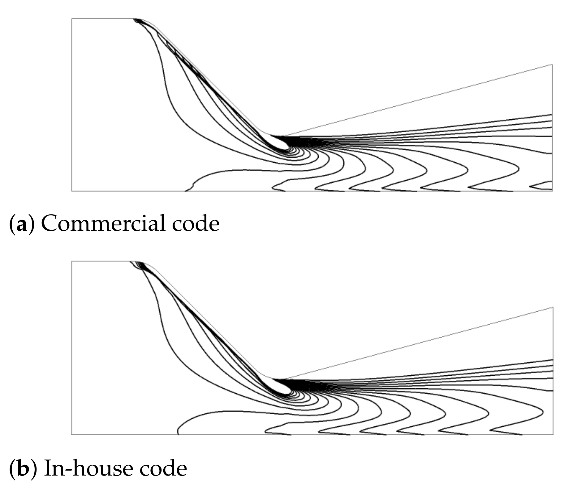
7.3. Two-Phase Flow in a Transonic Nozzle Configuration

Validation against commercial code results is carried out based on a geometry published by the Jet Propulsion Laboratory (JPL) located at the California Institute of Technology [37]. The flow is a dilute two-phase flow in a converging-diverging nozzle. Two-phase flow investigations have been published by [38,39,40]. The overall geometry is given in Figure 5 and is discretized using 4655 structured hexahedra elements.

At the inlet, the total conditions are set to $p_0^c=10.34$ bar and $T_0^c=555$ K for the continuous phase. The dispersed particle phase uses the same static pressure at the inlet as the continuous gas phase with a mass fraction of ${\mathsf{\Psi }}^d=0.3$. At the outlet, supersonic conditions are applied, accelerating the dilute two-phase flow to transonic conditions through the nozzle. The energy equation is solved for the continuous gas phase using ideal gas state equation, while the particles are assumed isothermal and incompressible with a density of ${\rho }^d=4004.62$ kg/m${}^3$. The two fluids are assumed inviscid with the viscosity in the drag term being defined using Sutherland’s law as given in Equation (51).

$$\begin{array}{c}\hfill {\mu }^c=1.458e^6\frac{T^c\sqrt{T^c}}{T^c-110.4}\end{array}$$

(51)

As shown in [39], two different particle sizes have been chosen. The first particles have a radius of 1 µm and the second simulation uses particles of $r_p=10$ µm. Figure 6 shows the results for the smaller particles and Figure 7 the results with the bigger particles. Both results compare well with commercial code results. Unphysical oscillations as visible at the symmetry plane of the commercial code results are not present for the proposed method. As expected, the lighter small particles follow the strong curvature of the converging-diverging nozzle section, the heavier particles tend to generate a particle free zone in the diverging section of the nozzle.

A comparison of the root mean square (RMS) error of the residual for the case of $r_p=1$ µm is shown in Figure 8. Both simulations are started with uniform initialization, upwind advection scheme, a time step of $\Delta t=1e^{-3}$ s and have been run using double precision. Double precision is requested from the commercial code whenever multiphase calculations are performed. This originates from the fact, that the volume fraction can attain very small values but still be of importance to the numerical results. While both codes initially close the outlet due to flow reversal occurring from the non-initialized conditions, the in-house framework recovers quickly from this situation. The problematic convergence behavior of commercial code up to iteration 600 is related to this closed faces at the outlet. However, after having recovered, it takes another 600 iterations to arrive at the supersonic conditions. Only thereafter, the simulation starts to convergence quickly.

The coupled framework was introduced in Section 4. A method is proposed that solves the two sets of momentum equations and the continuity equation in a 7 × 7 block matrix structure. It was later explained in Section 5.1 how this framework allows to treat inter phase drag implicitly in the coefficient matrix. The coupled drag formulation is therefore compared to traditional semi-implicit, segregated treatment of the drag term. In order to to so, the coefficients marked in blue in Equation (13) are entirely moved to the right hand side of the linearized equation system. The comparison therefore only differs in the treatment of the drag term, any other coupling is kept and the setup of the test case is identical. The results shown in Figure 9 clearly demonstrate the advantages of the proposed solutions. The RMS-residuals of the implicit formulation shown in the figure to the right outperform the explicit formulation.

8. Conclusions

A new formulation of the classical Rhie–Chow interpolation method was presented. The proposed solution takes advantage of a coupled formulation of multiphase momentum equations. The new formulation accounts implicitly and consistently for the drag body forces. In addition to yielding improved convergence and more accurate results, this coupled approach can be readily implemented in existing codes for multiphase flow simulation. The main modifications is in the computation of the inverted coefficient matrix, while computational memory requirements remain unchanged. The algorithm is first compared against analytical solution, showing the consistency of the implementation. The second testcase demonstrates the benefits of the consistent, coupled formulation compared to the original Rhie–Chow formulation. Finally, a transonic nozzle configuration was chosen and results were compared against commercial code to demonstrate the quality of the framework. The coupled formulation was then compared against the traditional segregated formulation of the drag term. Superior convergence behavior of the proposed approach was demonstrated. With the current derivations being limited here to two-phase flows, extension to any number of fluids is straightforward.

References

1. Hirt, C.W.; Nichols, B.D. Volume of fluid (VOF) method for the dynamics of free boundaries. J. Comput. Phys. 1981, 39, 201–225. [Google Scholar] [CrossRef]
2. Saurel, R.; Abgrall, R. A simple method for compressible multifluid flows. SIAM J. Sci. Comput. 1999, 21, 1115–1145. [Google Scholar] [CrossRef]
3. Miller, T.F.; Schmidt, F. Use of a pressure-weighted interpolation method for the solution of the incompressible Navier–Stokes equations on a nonstaggered grid system. Numer. Heat Transf. Part A Appl. 1988, 14, 213–233. [Google Scholar]
4. Osher, S.; Sethian, J.A. Fronts propagating with curvature-dependent speed: Algorithms based on Hamilton-Jacobi formulations. J. Comput. Phys. 1988, 79, 12–49. [Google Scholar] [CrossRef] [Green Version]
5. Olsson, E.; Kreiss, G. A conservative level set method for two phase flow. J. Comput. Phys. 2005, 210, 225–246. [Google Scholar] [CrossRef]
6. Kothe, D.B.; Rider, W.J. Comments on Modeling Interfacial Flows with Volume-of-Fluid Methods; Technical Report; Los Alamos National Laboratory: Los Alamos, NM, USA, 1995.
7. Sussman, M.; Puckett, E.G. A coupled level set and volume-of-fluid method for computing 3D and axisymmetric incompressible two-phase flows. J. Comput. Phys. 2000, 162, 301–337. [Google Scholar] [CrossRef] [Green Version]
8. Gerber, A. Two-phase Eulerian/Lagrangian model for nucleating steam flow. J. Fluids Eng. 2002, 124, 465–475. [Google Scholar] [CrossRef]
9. Kermani, M.; Gerber, A. A general formula for the evaluation of thermodynamic and aerodynamic losses in nucleating steam flow. Int. J. Heat Mass Transf. 2003, 46, 3265–3278. [Google Scholar] [CrossRef]
10. Gerber, A.; Kermani, M. A pressure based Eulerian–Eulerian multi-phase model for non-equilibrium condensation in transonic steam flow. Int. J. Heat Mass Transf. 2004, 47, 2217–2231. [Google Scholar] [CrossRef]
11. Van Wachem, B.; Almstedt, A.E. Methods for multiphase computational fluid dynamics. Chem. Eng. J. 2003, 96, 81–98. [Google Scholar] [CrossRef]
12. Badreddine, H.; Sato, Y.; Niceno, B.; Prasser, H.M. Finite size Lagrangian particle tracking approach to simulate dispersed bubbly flows. Chem. Eng. Sci. 2015, 122, 321–335. [Google Scholar] [CrossRef]
13. Kunz, R.F.; Siebert, B.W.; Cope, W.K.; Foster, N.F.; Antal, S.P.; Ettorre, S.M. A coupled phasic exchange algorithm for three-dimensional multi-field analysis of heated flows with mass transfer. Comput. Fluids 1998, 27, 741–768. [Google Scholar] [CrossRef]
14. Patankar, S.V.; Spalding, D.B. A calculation procedure for heat, mass and momentum transfer in three-dimensional parabolic flows. Int. J. Heat Mass Transf. 1972, 15, 1787–1806. [Google Scholar] [CrossRef]
15. Spalding, D. Developments in the IPSA procedure for numerical computation of multiphase-flow phenomena with interphase slip, unequal temperatures, etc. Numer. Prop. Methodol. Heat Transf. 1983, 421–436. [Google Scholar]
16. Spalding, D.B. Numerical computation of multi-phase fluid flow and heat transfer. In Von Karman Inst. for Fluid Dyn. Numerical Computation of Multi-Phase Flows; Pineridge Press: Swansea, UK, 1981; pp. 161–191. [Google Scholar]
17. Miller, T.F.; Miller, D.J. A Fourier analysis of the IPSA/PEA algorithms applied to multiphase flows with mass transfer. Comput. Fluids 2003, 32, 197–221. [Google Scholar] [CrossRef]
18. Lo, S. Mathematical Basis of A Multi-Phase Flow Model; Report: AEA Technology Plc; UKAEA Atomic Energy Research Establishment Thermal Hydraulics Division: Abingdon-on-Thames, UK, 1989.
19. Mangani, L.; Buchmayr, M.; Darwish, M. Development of a novel fully coupled solver in OpenFOAM: Steady-state incompressible turbulent flows in rotational reference frames. Numer. Heat Transf. Part Fundam. 2014, 66, 526–543. [Google Scholar] [CrossRef]
20. Mangani, L.; Darwish, M.; Moukalled, F. An OpenFOAM pressure-based coupled CFD solver for turbulent and compressible flows in turbomachinery applications. Numer. Heat Transf. Part Fundam. 2016, 69, 413–431. [Google Scholar] [CrossRef]
21. Yeoh, G.H.; Tu, J. Computational Techniques for Multiphase Flows; Butterworth-Heinemann: Oxford, UK, 2019. [Google Scholar]
22. Karema, H.; Lo, S. Efficiency of interphase coupling algorithms in fluidized bed conditions. Comput. Fluids 1999, 28, 323–360. [Google Scholar] [CrossRef]
23. Mangani, L. Development and Validation of an Object Oriented CFD Solver for Heat Transfer and Combustion Modelling in Turbomachinery Applications. Ph.D. Thesis, Dipartimento di Energetica, Università degli Studi di Firenze, Florence, Italy, 2008. [Google Scholar]
24. Hanimann, L.; Mangani, L.; Casartelli, E.; Vogt, D.M.; Darwish, M. Real Gas Models in Coupled Algorithms Numerical Recipes and Thermophysical Relations. Int. J. Turbomach. Propuls. Power 2020, 5, 20. [Google Scholar] [CrossRef]
25. Schiller, L. A drag coefficient correlation. Zeit. Ver. Deutsch. Ing. 1933, 77, 318–320. [Google Scholar]
26. Rhie, C.; Chow, W. Numerical study of the turbulent flow past an airfoil with trailing edge separation. AIAA J. 1983, 21, 1525–1532. [Google Scholar] [CrossRef]
27. Majumdar, S. Role of underrelaxation in momentum interpolation for calculation of flow with nonstaggered grids. Numer. Heat Transf. 1988, 13, 125–132. [Google Scholar] [CrossRef]
28. Choi, S.K. Note on the use of momentum interpolation method for unsteady flows. Numer. Heat Transf. Part A Appl. 1999, 36, 545–550. [Google Scholar] [CrossRef]
29. Choi, S.K.; Kim, S.O.; Lee, C.H.; Choi, H.K. Use of the momentum interpolation method for flows with a large body force. Numer. Heat Transf. Part B Fundam. 2003, 43, 267–287. [Google Scholar] [CrossRef]
30. Yu, B.; Tao, W.Q.; Wei, J.J.; Kawaguchi, Y.; Tagawa, T.; Ozoe, H. Discussion on momentum interpolation method for collocated grids of incompressible flow. Numer. Heat Transf. Part B Fundam. 2002, 42, 141–166. [Google Scholar] [CrossRef]
31. Cubero, A.; Fueyo, N. A compact momentum interpolation procedure for unsteady flows and relaxation. Numer. Heat Transf. Part B Fundam. 2007, 52, 507–529. [Google Scholar] [CrossRef]
32. Cubero, A.; Sánchez-Insa, A.; Fueyo, N. A consistent momentum interpolation method for steady and unsteady multiphase flows. Comput. Chem. Eng. 2014, 62, 96–107. [Google Scholar] [CrossRef]
33. Ferreira, G.G.; Lage, P.L.; Silva, L.F.L.; Jasak, H. Implementation of an implicit pressure–velocity coupling for the Eulerian multi-fluid model. Comput. Fluids 2019, 181, 188–207. [Google Scholar] [CrossRef]
34. Morsi, S.; Alexander, A. An investigation of particle trajectories in two-phase flow systems. J. Fluid Mech. 1972, 55, 193–208. [Google Scholar] [CrossRef]
35. Moukalled, F.; Darwish, M. A comparative assessment of the performance of mass conservation-based algorithms for incompressible multiphase flows. Numer. Heat Transf. Part B Fundam. 2002, 42, 259–283. [Google Scholar] [CrossRef]
36. Darwish, M.; Abdel Aziz, A.; Moukalled, F. A coupled pressure-based finite-volume solver for incompressible two-phase flow. Numer. Heat Transf. Part B Fundam. 2015, 67, 47–74. [Google Scholar] [CrossRef]
37. Back, L.; Cuffel, R. Detection of oblique shocks in a conical nozzle with a circular-arc throat. AIAA J. 1966, 4, 2219–2221. [Google Scholar] [CrossRef]
38. Chang, H.T.; Hourng, L.W.; Chien, L.C.; Chien, L.C. Application of flux-vector-splitting scheme to a dilute gas–particle jpl nozzle flow. Int. J. Numer. Methods Fluids 1996, 22, 921–935. [Google Scholar] [CrossRef]
39. Darwish, M.; Moukalled, F.; Sekar, B. A robust multi-grid pressure-based algorithm for multi-fluid flow at all speeds. Int. J. Numer. Methods Fluids 2003, 41, 1221–1251. [Google Scholar] [CrossRef]
40. Moukalled, F.; Darwish, M.; Sekar, B. A pressure-based algorithm for multi-phase flow at all speeds. J. Comput. Phys. 2003, 190, 550–571. [Google Scholar] [CrossRef]
Figure 1. Morsi–Alexander Case Setup.
Ijtpp 06 00007 g001
Figure 2. Dilute Gas–Solid Flow: Comparison against analytical solution and reference results of [36].
Ijtpp 06 00007 g002
Figure 3. Triangular 2D obstacle.
Ijtpp 06 00007 g003
Figure 4. Effects on the r c -field for r c ∈ [0.9636 ⋯ 1].
Ijtpp 06 00007 g004
Figure 5. Jet Propulsion Laboratory (JPL) nozzle geometry.
Ijtpp 06 00007 g005
Figure 6. Particle radius r p = 1 µm, r p ∈ [7.2 · 10−5 ⋯ 0.001].
Ijtpp 06 00007 g006
Figure 7. Particle radius r p = 10 µm, r p ∈ [7.2 · 10−5 ⋯ 0.001].
Ijtpp 06 00007 g007
Figure 8. Root mean square (RMS) residual error for r d = 1 µm with different numerical frameworks.
Ijtpp 06 00007 g008
Figure 9. Root mean square (RMS) residual error for r d = 1 µm with different momentum interpolation.
Ijtpp 06 00007 g009
Publisher’s Note: MDPI stays neutral with regard to jurisdictional claims in published maps and institutional affiliations.