Article

Scale-Resolving Hybrid RANS-LES Simulation of a Model Kaplan Turbine on a 400-Million-Element Mesh †

by
Simon Joßberger
* and
Stefan Riedelbauch
Institute of Fluid Mechanics and Hydraulic Machinery, University of Stuttgart, Pfaffenwaldring 10, 70569 Stuttgart, Germany
*
Author to whom correspondence should be addressed.
This manuscript is an extended version of the ETC2023-343 meeting paper published in the Proceedings of the 15th European Turbomachinery Conference, Budapest, Hungary, 24–28 April 2023.
Int. J. Turbomach. Propuls. Power 2023, 8(3), 26; https://doi.org/10.3390/ijtpp8030026
Submission received: 18 June 2023 / Revised: 17 July 2023 / Accepted: 20 July 2023 / Published: 2 August 2023

Abstract

:
Double-regulated Kaplan turbines with adjustable guide vanes and runner blades offer a high degree of flexibility and good efficiency for a wide range of operating points. However, this also leads to a complex geometry and flow guidance with, for example, vortices of different sizes and strengths. The flow in a draft tube is especially challenging to simulate mainly due to flow phenomena, like swirl, separation and strong adverse pressure gradients, and a strong dependency on the upstream flow conditions. Standard simulation approaches with RANS turbulence models, a coarse mesh and large time step size often fail to correctly predict performance and can even lead to wrong tendencies in the overall behavior. To reveal occurring flow phenomena and physical effects, a scale-resolving hybrid RANS-LES simulation on a block structured mesh of about 400 million hexahedral elements of a double-regulated five-blade model Kaplan turbine is carried out. In this paper, first, the results of the ongoing simulation are presented. The major part of the simulation domain is running in LES mode and seems to be properly resolved. The validation of the simulation results with the experimental data shows mean deviations of less than 0.8% in the global results, i.e., total head and power, and a good visual agreement with the three-dimensional PIV measurements of the velocity in the cone and both diffuser channels of the draft tube. In particular, the trend of total head and the results for the draft tube differ significantly between the scale-resolving simulation and a standard RANS simulation. The standard RANS simulation exhibits a highly unsteady behavior of flow, which is not observed in the experiments or scale-resolving simulation.

1. Introduction

The increasing use of volatile renewable energies, like wind and solar power, has led to higher fluctuations of available power in the electricity grid. Hydropower, as a predictable and reliable source of electricity, can be used to compensate the fluctuating power output and stabilize the energy grid. Double-regulated Kaplan turbines with adjustable guide vanes and runner blades offer high efficiency over a wide range of operating points. This wide operational flexibility requires a substantial change in the runner blade opening. The gaps on both the tip and hub of the runner blades create flow vortices interacting with the decelerated flow of the draft tube. The flow in a draft tube is especially challenging to simulate due to flow phenomena, like swirl, separation and strong adverse pressure gradients (cf. [1]), and a strong dependency on the flow conditions at the inlet defined by the quality and fidelity of the simulation upstream (cf. [2]). Typical Kaplan turbines are applied for small to medium heads. Therefore, even small errors in flow-dependent losses can lead to wrong predictions of performance and overall operating range.
The overall goal of this ongoing investigation is to detect and understand occurring flow phenomena and identify their importance to accurately simulate Kaplan turbines. To achieve this, a highly resolved simulation with a hybrid RANS-LES turbulence model on a very fine mesh with about 400 million hexahedral elements is carried out. Advanced turbulence models have demonstrated an improvement in the results and level of detail (cf. [3,4,5,6,7]), but their numerical requirements, e.g., time step size and mesh resolution, have been generally much higher than standard RANS simulation approaches and typically too costly for industrial development processes. A comparison of the high-resolution simulation with different less complex simulations allows for the identification of important flow phenomena and how standard simulation approaches and development processes can be improved. To validate the simulation results, time-averaged experimental values for the total head and power of the runner are available, as well as phase-resolved three-dimensional PIV measurements in a plane just downstream of the runner and in a plane in each of the two diffuser channels of the draft tube. The details of the experimental investigation were published in [8].
In this part of the study, an estimation of the achieved numerical resolution and first results of the high-resolution simulation are described. Furthermore, a comparison of the experimental data and a standard RANS simulation on a mesh with 20 million hexahedral elements is presented. This manuscript is an extended version of the ETC2023-343 meeting paper published in the Proceedings of the 15th European Turbomachinery Conference, Budapest, Hungary, 24–28 April 2023 [9].

2. Numerical Setup and Model Turbine

The investigated turbine is a Kaplan turbine in model scale. The whole simulation domain consists of five subdomains (cf. Figure 1) and begins with the rectangular semi spiral intake, which includes two piers. The following subdomain consists of 23 stay vanes and 24 adjustable guide vanes. The runner consists of a hub and five adjustable blades. No geometric simplifications are used for the runner blades. Both the tip and hub clearance and the fillets between the runner blades and the hub are modeled. The currently investigated operating point is an on-cam point, where the pitch angles of guide vanes and runner blades are matched. An elbow-type draft tube with one pier leads to the tailwater tank. The geometry of the tailwater tank matches the model test arrangement at the hydraulic laboratory. The outlet of the simulation domain is defined at the end of the pipe downstream of the tailwater tank. This minimizes the impact of the boundary conditions on the flow in the draft tube and allows an accurate evaluation of results even at the end of the draft tube. Due to the fact that the flow in the tailwater tank is of no particular interest, the tailwater tank will be neglected in the following Section 3.
ICEM CFD is utilized to generate the block-structured hexahedral mesh with about 20 and 400 million elements for the standard RANS approach and the high-resolution simulation, respectively. The main differences between the 20 million element (20 M) and 400 million element (400 M) meshes are in the resolution of the boundary layer and overall element size while preserving the distribution of elements as much as possible. To properly resolve the boundary layer without the use of wall functions, a fine mesh at the wall, and a small growth rate normal for the wall is required (cf. Figure 2). With an unchanged overall element size, this leads to a mesh with about 50 million elements. For the 400 M mesh, the element size is additionally approximately halved in all directions while maintaining the general block structure as much as possible. The number of cells in the five subdomains intake with semi spiral casing (SC), stay and guide vanes (SVGVs), runner (RU), draft tube (DT) and tailwater tank (TW) for both meshes is listed in Table 1.
The simulations are conducted with ANSYS CFX, version 19.5. Automatic wall treatment is activated for the boundary layer (cf. [10]). Depending on the local dimensionless wall distance, y + , either wall functions or the direct calculation of the boundary layer is applied (cf. Figure 2). The average and maximum values and the 95th percentile of the time-averaged y + values of the subdomains neglecting the tailwater tank are listed in Table 2. In the 20 M simulation the average y + -value ranges between 57 and 82 depending on the subdomain. This leads to the use of wall functions. As indicated by the 95th percentile and the average, most of the elements of the 400 M simulation have a y + -value smaller than 2. This should lead to direct calculation of the boundary layer in most parts of the domain. In both simulations, the same time-averaged three-dimensional distributions of velocity and turbulence properties from a preceding unsteady simulation of the flow in the head water tank are specified as inlet boundary conditions (cf. [8,11]). An average static pressure is set as the outlet boundary condition. General grid interfaces (GGIs) are employed between stationary subdomains. Full 360° transient rotor–stator interfaces connect the rotating runner subdomain with the stationary stay vane and draft tube subdomain.
Turbulence is modeled by the RANS k ω shear-stress transport (SST) model for the 20 M simulation and by the hybrid RANS-LES stress-blended eddy simulation (SBES) model for the 400 M simulation. The SST model combines the advantages of the k ω model in wall-bounded flows with the advantages of the k ϵ model in free shear flows (cf. [12]). It is a standard RANS model and is commonly applied in simulating hydraulic turbomachinery. The SBES model uses an unpublished shielding function, f S , to blend between the stress tensor, τ i j , modeled by the RANS and LES model (cf. [13]):
τ i j S B E S = f S τ i j R A N S + ( 1 f S ) τ i j L E S
In this study, the SST model and the wall-adapted local eddy viscosity model (WALE) are used for the RANS and LES parts, respectively. Compared to other hybrid RANS-LES approaches, the SBES model has the advantage of a quick transition from RANS to LES mode and a clear distinction between both regions by the shielding function, f S (cf. [14]).
For spatial discretization, the high-resolution scheme is applied for the SST simulation, and a bounded central differencing scheme is used for the SBES simulation (cf. [10]). A second-order backward Euler scheme is employed for temporal discretization in all simulations (cf. [14]). A fixed number of five inner loops per time step is used. With the final time step size, this leads to maximum root mean square values of the residuals of about 8.0 × 10 6 and 1.5 × 10 4 in the 20 M and 400 M simulations, respectively. A time step size of Δ t = 2 × 10 4 s , which is equivalent to a 1.8 ° runner revolution, is used for the 20 M simulation. This is a typical order of magnitude for unsteady RANS simulations of hydropower turbines. The unsteady simulation is initialized with a steady-state SST simulation on the same mesh. Due to numerical instabilities, the 400 M simulation can not be initialized with a steady-state simulation, and the results of a preceding unsteady simulation have to be used. In theory, the build-up time necessary to obtain statistically valid results can be reduced by a higher quality of initial conditions. Therefore, an unsteady simulation with the SBES turbulence model on the 20-million-element mesh and a time step size of Δ t = 1 × 10 4 s , equivalent to a 0.9 ° runner revolution, is used as the initial conditions. After 10 revolutions, the time step size is ramped down to Δ t = 5 × 10 5 s over the course of about 100 iterations. After an additional five revolutions, the time step size is ramped down to a final value of Δ t = 2.5 × 10 5 s , equivalent to 1.225 ° of runner revolution.
For both simulations, the averaging of data and the evaluation of results are started after a build-up time of 20 revolutions. This is equivalent to 4000 and 15,920 time steps in the 20 M and 400 M simulations, respectively, and corresponds to about two convective flows from the inlet of the semi spiral casing to the outlet of the draft tube. The number of build-up iterations is chosen by experience with similar simulations of hydropower turbines and by the trend of integral values of interest in the subdomains. Due to the unsteady behaviour of the flow in the draft tube in the 20 M simulation, this subdomain is less suited for the consideration of build-up time.

3. Results

In the following sections, the 20 build-up revolutions are neglected and only results of the subsequent revolutions are presented.

3.1. Estimation of Achieved Resolution in the 400 M Simulation

To derive the RANS equations of the Navier–Stokes equations, the flow variables are decomposed into a mean or time-averaged component and a fluctuating turbulent component. Since the latter component and the resulting turbulence energy cascade is almost completely modeled by the turbulence model, the time step size of an unsteady RANS simulation is, in theory, sufficiently small when it is able to capture the unsteady fluctuations of the mean values excited by external influences, such as interactions between the guide vanes and runner blades. In contrast to this, in an LES simulation, all but the smallest turbulent scales are directly simulated. To avoid excessive damping of turbulence in the LES region, [14] recommends a Courant number of C F L 1 or smaller.
In Table 3, the average and maximum values and the 95th percentile of the time-averaged Courant number are presented. The values for the 400 M simulation are divided into the LES region and the RANS region. In the LES region of all subdomains, the average Courant number is smaller than 1, and most of the elements have a Courant number smaller than 2, as indicated by the 95th percentile. The left part of Figure 3 shows the root mean square of about 30 revolutions of the Courant number on a cut through the turbine for the 400 M simulation. The areas exceeding the recommendation of C F L 1 are mostly in regions with a fine mesh resolution, like leading and trailing edges and the gaps of the runner blades. The time step size would have to be approximately halved to achieve a Courant number smaller than 1 for almost all elements. This would, in turn, approximately double the computing time for one revolution. With the used time step size, one revolution requires about 240,000 core hours or about 2.5 days wall-clock time on 4096 cores at the High Performance Computing Center Stuttgart. Hence, the selected final time step size of the 400 M simulation is a compromise between accuracy and feasibility.
The shielding function, f S , of the SBES turbulence model is used to visualize whether the RANS or LES model is used. The black lines in the right picture of Figure 3 represent a value of f S = 0.99 , and the magenta lines represent a value of f S = 0.01 . The regions outside the black lines are basically completely in RANS mode, while the regions inside the magenta lines are in LES mode. The small regions in-between the lines are the transition zones between the two models. The transition from RANS to LES primarily occurs in the semi spiral casing and stay and guide vanes. Downstream of the guide vanes, almost all of the simulation domain is in LES mode. In the runner and draft tube, only the boundary layer is in RANS mode, while all other areas are in LES mode. This is the intended state for a hybrid RANS-LES simulation. In the LES region, the amount of modeled turbulence, depicted by the eddy viscosity ratio, ν t / ν , built with the turbulent viscosity, ν t , and the dynamic viscosity, ν , is quite small. In the RANS region, the viscosity ratio is about two orders of magnitude higher. This can also be seen in Figure 4, where the resolved turbulent structures in the draft tube are visualized. The turbulent structures are depicted by an isosurface of the second invariant of the velocity gradient tensor, Q = 0.5 | | Ω | | 2 | | S | | 2 = 50 , built with the vorticity tensor, Ω = 0.5 ( u i / u j u j / u i ) , and the strain rate tensor, S = 0.5 ( u i / u j + u j / u i ) , and colored by the viscosity ratio. Compared to the 20 M simulation, the 400 M simulation resolves much finer structures and calculates the energy transfer due to turbulence on a much finer scale.

3.2. Comparison of Simulations and Measurement

The left part of Figure 5 shows the power and the right part the total head of the 20 M and 400 M simulation relative to the measurement. Both simulations match the measured power very well, with a little advantage for the 20 M simulation. The power trend of the 20 M simulation exhibits only minor oscillations without high random deflections. In comparison, the power trend of the 400 M simulation shows slightly higher oscillations and an overall noisier behavior. This is probably an effect of the higher temporal and spatial resolutions and the ability of the SBES model to resolve much smaller turbulent structures. Nonetheless, the power trend of both simulations reached a quasi steady state. The trend of the total head exhibits a different behavior. The result for the 400 M simulation is in good agreement with the measurement and reached a quasi steady state, which was also observed in the experiment. The trend of the 20 M simulation is highly unsteady and overestimates the head by more than 6 % at the maximum. During the course of 50 additionally calculated but not shown revolutions, the trend does not settle and, therefore, seems to be not a singular event but normal behavior for this simulation approach.
Figure 6 shows an instantaneous circumferential velocity field on the measurement plane in the cone of the draft tube just downstream of the runner blades. Basic flow features, e.g., the wake of the runner blades, are visible in both simulations and the measurement. However, the 20 M simulation shows a very smooth flow field. The level of detail is much higher for the 400 M simulation and the measurement, where small flow features are resolved. The granularity and magnitude of the resolved flow features are quite comparable between the 400 M simulation and the measurement.
Figure 7 shows the time-averaged velocity and corresponding standard deviation on the measurement plane in the left diffuser channel of the draft tube. The underlying data used to build the time-averaged flow field are quite different between simulations and the measurement. In the simulations, all time steps of about 30 revolutions are used, leading to 30 × 200 = 6000 and 30 × 1600 = 48,000 individual data sets in the 20 M and 400 M simulations, respectively. The measurement consists of 1000 revolutions, but only nine data sets per revolution are taken with a time lag equivalent to an 8 ° runner revolution between subsequent data sets. This leads to a total of 9000 data sets. Despite the different data basis, the results of the 400 M simulation and the measurement are in good agreement. Both velocity and standard deviation show a similar distribution and pattern, as well as comparable magnitudes. The velocity distribution of the 20 M simulation differs and exhibits a much more unsteady behavior, as can be seen by the higher standard deviation. The data of the measurement plane in the right diffuser channel exhibit comparable results and are, therefore, not presented.

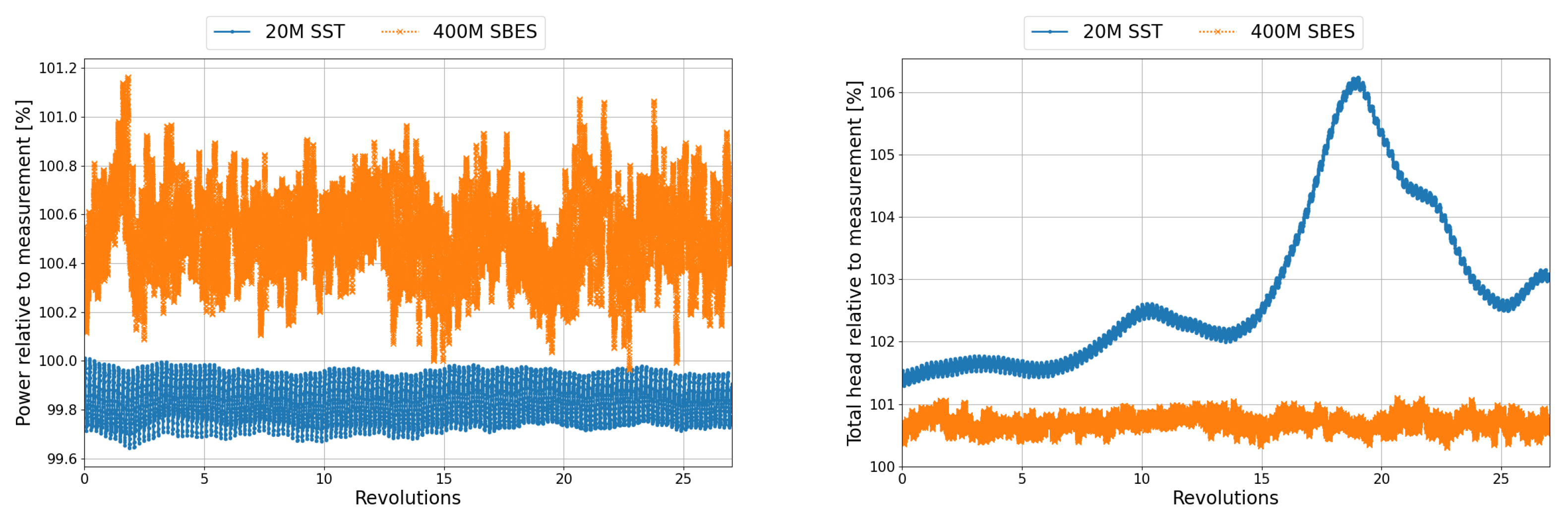
3.3. Comparison of Time-Resolved Results for 20 M and 400 M Simulations

To identify the origin of the unsteady trend of the total head (cf. Figure 5), the head losses of the individual subdomains normalized with the corresponding mean of the 400 M simulation are shown in Figure 8. It is evident that the unsteady behavior of the total head in the 20 M simulation is mostly determined by the losses in the draft tube. The other subdomains exhibit a more or less constant course similar to the power and reach quasi steady states. In comparison to the 400 M simulation, the losses in the 20 M simulation are higher in all subdomains but show smaller oscillations.
The origin of the unsteady losses in the draft tube are further isolated with the help of monitor planes. Specific variables, like velocity and pressure, are saved for every iteration on different monitor planes in the turbine. The monitor planes used in the following analysis are shown in Figure 9 and are located in downstream direction as follows: Runner Out is a monitor plane just downstream of the runner blades at the beginning of the draft tube cone. Cone Out is at the end of the cone and at the transition to the elbow. DT Left In and DT Right In are near the inlet to the left and right diffuser channels of the draft tube. DT Left Out and DT Right Out are at the outlet of the left and right diffuser channels.
Figure 10 shows the mass-flow-averaged kinetic energy and pressure on the monitor planes. The trend of kinetic energy on the monitor plane Cone Out of the 20 M simulation correlates very well with the trend of head loss in the draft tube in Figure 8. An increase in kinetic energy leads to an increase in head loss. The change in kinetic energy is transported downstream to the diffuser channels with a time delay. No upstream influence on the runner is observed. At the outlet of the draft tube, the disturbance has mostly subsided. The trend of pressure shows a similar behavior with two major differences. The first difference is that the two diffuser channels exhibit an opposing trend. An increase in pressure in the cone leads to a time-delayed increase in the left channel and a time-delayed decrease in the right channel. The second difference is that a change in pressure in the cone leads to a time-delayed opposing change in pressure in the upstream direction. The shown results lead to the conclusion that the unsteady behavior of the draft tube originates in the cone of the draft tube.
This conclusion is further confirmed by Figure 11, where instantaneous velocity fields are shown on multiple monitor planes in the draft tube for different revolutions. For revolution five, the head loss in the draft tube (cf. Figure 8) has a similar value for both the 20 M and 400 M simulations. The flow field in the draft tube is largely comparable. Extensive flow features, e.g., higher velocities at the top than the bottom of the elbow, are present in both simulations. In detail, there are differences. These are particularly visible on the plane at the end of the cone. The 20 M simulation shows a region of low velocity near the wall, which is not present in the 400 M simulation. Furthermore, the overall granularity is much finer in the 400 M simulations. The following shown revolutions from 15 to 25 comprise the major peak in the trend of the total head and head loss in the draft tube of the 20 M simulation. The 400 M simulation does not change drastically with time. Major flow features remain preserved, and only spatial limited fluctuations occur. The flow of the 20 M simulation exhibits a substantially different behavior. Starting with revolution 15, the region with low velocities at the end of the cone becomes unstable and detaches from the wall in the following revolutions. In the last two shown pictures, the flow in the cone stabilizes again. The detachment is transported downstream and leads to major vortices downstream of the cone, which is especially visible on the monitor plane in the elbow. With increasing distance in the downstream direction, the impact of the detachment on the flow field weakens. At the outlet of the draft tube, only minor changes in the flow field are visible. The flow upstream at the inlet to the cone is only slightly influenced. The shown instability explains the differences in velocity and standard deviation on the measurement planes in the diffuser channels between the 20 M simulation, 400 M simulation and measurement shown in Figure 7.

4. Conclusions and Outlook

The first results of a hybrid RANS-LES simulation on a mesh with 400 million hexahedral elements and of a standard RANS simulation with 20 million hexahedral elements were presented and compared to each other as well as measurements. The results of the 400 M simulation indicate that most of the simulation domain ran in LES mode and that the regions in LES mode were properly resolved. Furthermore, the results are in good agreement with the measurement, and the simulation seems to accurately predict the flow in the turbine. A time-resolved analysis of the 400 M simulation shows that this simulation reached a quasi steady state in the integral values and flow field, which was also observed in the experiment. The 20 M simulation exhibited a highly unsteady behavior in the draft tube, leading to an unsteady trend of the total head. This instability arose in the cone of the draft tube and was transported primarily in downstream direction.
Currently, the most crucial flow features and primary influencing factors for precise simulations of Kaplan turbines, such as the turbulence model and time step size, remain unclear. In order to determine these factors, a comprehensive analysis is required, which involves comparing current simulations and experiments and conducting additional simulations with varied settings.

Author Contributions

Conceptualization, S.J. and S.R.; methodology, S.J. and S.R.; software, S.J.; validation, S.J. and S.R.; formal analysis, S.J.; investigation, S.J.; resources, S.J. and S.R.; data curation, S.J.; writing—original draft preparation, S.J.; writing—review and editing, S.J. and S.R.; visualization, S.J.; supervision, S.R.; project administration, S.J. and S.R.; funding acquisition, S.R. All authors have read and agreed to the published version of the manuscript.

Funding

This research received no external funding.

Data Availability Statement

Restrictions apply to the availability of the data presented in this study. Data are available on request from the authors with prior permission of Voith Hydro Holding GmbH.

Acknowledgments

The research leading to the results presented in this paper was part of a common research project of the University of Stuttgart and Voith Hydro Holding GmbH. The authors thank the High Performance Computing Center Stuttgart for the support and supply of computation time. The authors thank Euroturbo for covering the Journal publication costs.

Conflicts of Interest

The authors declare no conflict of interest.

Nomenclature and Abbreviations

y + Dimensionless wall distance
Δ t       Time step size
ν t Turbulent viscosity
ν Dynamic viscosity
f S Shielding function of SBES turbulence model
QQ-criterion—second invariant of the velocity gradient tensor
SStrain rate tensor
Ω Vorticity tensor
20 MSimulation on a 20-million-element mesh
400 MSimulation on a 400-million-element mesh
RANSReynolds-averaged Navier–Stokes (equation)
LESLarge eddy simulation
SBESStress-blended eddy simulation
PIVParticle image velocimetry
SCSpiral casing
SVGVStay vane and guide vane
RURunner
DTDraft tube
TWTailwater

References

  1. Cervantes, M.; Engstrom, T.; Gustavsson, L. Turbine-99 III. In Proceedings of the Third IAHR/ERCOFTAC Workshop on Draft Tube Flows, Porjus, Sweden, 8–9 December 2005. [Google Scholar]
  2. Nilsson, H.; Cervantes, M. Effects of the inlet boundary conditions, on the computed flow in the Turbine-99 draft tube, using OpenFOAM and CFX. IOP Conf. Ser. Earth Environ. Sci. 2012, 15, 032002. [Google Scholar] [CrossRef]
  3. Jošt, D.; Škerlavaj, A.; Lipej, A. Improvement of Efficiency Prediction for a Kaplan Turbine with advanced Turbulence Models. Stroj. Vestn./J. Mech. Eng. 2014, 60, 124–134. [Google Scholar] [CrossRef] [Green Version]
  4. Krappel, T.; Riedelbauch, S. Scale Resolving Flow Simulations of a Francis Turbine Using Highly Parallel CFD Simulations. High Perform. Comput. Sci. Eng. 2016, 16, 499–510. [Google Scholar]
  5. Krappel, T.; Riedelbauch, S.; Jester-Zuerker, R.; Jung, A.; Flurl, B.; Unger, F.; Galpin, P. Turbulence Resolving Flow Simulations of a Francis Turbine in Part Load using Highly Parallel CFD Simulations. High Perform. Comput. Sci. Eng. 2016, 49, 421–433. [Google Scholar] [CrossRef]
  6. Javadi, A.; Nilsson, H. Detailed numerical investigation of a Kaplan turbine with rotor-stator interaction using turbulence-resolving simulations. Int. J. Heat Fluid Flow 2017, 63, 1–13. [Google Scholar] [CrossRef]
  7. Minakov, A.; Platonov, D.; Litvinov, I.; Shtork, S.; Hanjalić, K. Vortex ropes in draft tube of a laboratory Kaplan hydroturbine at low load: An experimental and LES scrutiny of RANS and DES computational models. J. Hydraul. Res. 2017, 55, 668–685. [Google Scholar] [CrossRef] [Green Version]
  8. Beck, J.; Joßberger, S.; Jester-Zürker, R.; Riedelbauch, S. PIV measurements on a Kaplan turbine and comparison with scale-adaptive numerical analysis. IOP Conf. Ser. Earth Environ. Sci. 2019, 405, 012024. [Google Scholar] [CrossRef]
  9. Joßberger, S.; Riedelbauch, S. Scale resolving hybrid RANS-LES simulation of a model Kaplan turbine on a 400 million element mesh. In Proceedings of the 15th European Turbomachinery Conference, Paper N. ETC2023-343, Budapest, Hungary, 24–28 April 2023; Available online: https://www.euroturbo.eu/publications/conference-proceedings-repository (accessed on 17 June 2023).
  10. ANSYS Inc. ANSYS CFX-Solver Modeling Guide Release 19.5; Technical Report; ANSYS Inc.: Canonsburg, PA, USA, 2019. [Google Scholar]
  11. Joßberger, S.; Riedelbauch, S. Influence of the Inlet Boundary Conditions on Numerical Flow Simulations of a Model Kaplan Turbine. In Proceedings of the 13th European Conference on Turbomachinery, Fluid Dynamics and Thermodynamics, Lausanne, Switzerland, 8–12 April 2019. [Google Scholar]
  12. ANSYS Inc. ANSYS CFX-Solver Theory Guide Release 19.5; Technical Report; ANSYS Inc.: Canonsburg, PA, USA, 2019. [Google Scholar]
  13. Menter, F. Stress-Blended Eddy Simulation (SBES)—A new Paradigm in hybrid RANS-LES Modeling. Notes Numer. Fluid Mech. Multidiscip. Des. 2016, 137, 27–37. [Google Scholar]
  14. Menter, F. Best Practice: Scale-Resolving Simulations in ANSYS CFD—Version 2.0; Technical Report; ANSYS Germany GmbH: Darmstadt, Germany, 2015. [Google Scholar]
Figure 1. Simulation domain. Red: inlet area and semi spiral casing (SC). Blue: stay and guide vanes (SVGVs). Green: runner (RU). Orange: draft tube (DT). Yellow: tailwater tank (TW).
Ijtpp 08 00026 g001
Figure 2. Characteristic mesh distribution at the wall coloured by time-averaged velocity. (Left) A 20 M simulation with boundary layer wall function. (Right) A 400 M simulation with direct calculation of boundary layer.
Ijtpp 08 00026 g002
Figure 3. Cut through the turbine for 400 M simulation. (Left) Root mean square of Courant number. (Right) Viscosity ratio, ν t / ν , and shielding function, f S , of the SBES turbulence model (black line: f S = 0.99 ; magenta line: f S = 0.01 ).
Ijtpp 08 00026 g003
Figure 4. Instantaneous isosurface of velocity invariant Q = 0.5 | | Ω | | 2 | | S | | 2 = 50 to depict resolved turbulent structures colored by viscosity ratio, ν t / ν . Different scales are used for the viscosity ratio. (Left) 20 M simulation. (Right) 400 M simulation.
Ijtpp 08 00026 g004
Figure 5. Power (left) and total head (right) relative to measurements.
Ijtpp 08 00026 g005
Figure 6. Instantaneous circumferential velocity on the measurement plane in the draft tube cone. Values normalized with the maximum value of the 400 M simulation. (Left) 20 M simulation. (Middle) 400 M simulation. (Right) measurement.
Ijtpp 08 00026 g006
Figure 7. Time -veraged velocity (top row) and standard deviation (bottom row) on the measurement plane in the left diffuser channel. Values normalized with the maximum value of the 400 M simulation. (Left) 20 M simulation. (Middle) 400 M simulation. (Right) measurement.
Ijtpp 08 00026 g007
Figure 8. Head loss in individual subdomains relative to corresponding mean of the 400 M simulation. (Top left) spiral casing. (Top right) stay and guide vanes. (Bottom left) runner. (Bottom right) draft tube.
Ijtpp 08 00026 g008
Figure 9. Monitor planes in the draft tube.
Ijtpp 08 00026 g009
Figure 10. Mass-flow-averaged kinetic energy (left) and pressure (right) on different monitor planes in the draft tube (cf. Figure 9). The values are normalized with the respective value of Runner Out 400 M SBES.
Ijtpp 08 00026 g010
Figure 11. Instantaneous velocity fields on monitor planes in the draft tube at different revolutions. Left rows: 20 M simulation. Right rows: 400 M simulation.
Ijtpp 08 00026 g011aIjtpp 08 00026 g011b
Table 1. Number of cells of the subdomains in million elements.
SimTotalSCSVGVRUDTTW
20 M19.82.17.04.74.91.1
400 M399.529.878.663.3218.29.6
Table 2. Average, maximum and 95th percentile of time-averaged y + value in the subdomains.
SCSVGVRUDT
SimAveMaxp95AveMaxp95AveMaxp95AveMaxp95
20 M62.1145.199.981.7267.1132.957.0135.188.560.5221.3105.5
400 M0.541.860.890.5969.71.070.966.633.840.422.020.93
Table 3. Average, maximum and 95th percentile of time-averaged Courant number in the subdomains.
SCSVGVRUDT
SimAveMaxp95AveMaxp95AveMaxp95AveMaxp95
20 M0.072.780.171.2119.13.304.203589.230.3912.81.58
400 M RANS region0.021.010.041.291464.053.044239.590.085.250.33
400 M LES region0.030.600.080.811231.890.872201.770.113.360.26
Disclaimer/Publisher’s Note: The statements, opinions and data contained in all publications are solely those of the individual author(s) and contributor(s) and not of MDPI and/or the editor(s). MDPI and/or the editor(s) disclaim responsibility for any injury to people or property resulting from any ideas, methods, instructions or products referred to in the content.

