Surrogate Modeling of the Aeroacoustics of an NM80 Wind Turbine ^†

Abstract

Wind turbines play a major role in the European Green Deal for clean energy transition. Noise is a critical aspect among open technological issues, as it determines the possibility of onshore installations near inhabited places and the possible detrimental effects on wildlife when offshore. This paper assesses the accuracy of different approaches to predicting the sound pressure level (SPL) of a wind turbine. The 2.75 MW Neg Micon NM80 horizontal axis wind turbine (HWAT) was simulated in OpenFOAM, modeling the turbine with the actuator line method (ALM) implemented in the turbinesFoam library. Two different inflow conditions were considered: a stationary inflow with a typical atmospheric boundary layer profile and a time-dependent inflow derived from a precursor channel with fully turbulent conditions. The surrogate model for noise prediction used for this work is based on the synthetic/surrogate acoustics models (SAMs) of Amiet and Brooks-Pope-Marcolini (BPM). This approach allows for blade motion modeling and the prediction of the SPL of the URANS postprocessing results. The SPL spectrum obtained was then compared to the results from the other aeroacoustic solvers of IEA Task 39 participants, showing the best performance in the fully turbulent case. The results demonstrate that coupling between the ALM and surrogate acoustics provides more accurate results than the blade element momentum (BEM) approach.

1. Introduction

The European Green Deal for clean energy transition is the blueprint for shifting energy production from fossil fuels to renewable energy. Wind turbines (WTs) and, in particular, their offshore installations play a central role in renewable energy and clean energy transition. In fact, the European Commission has officially acknowledged that wind energy tops most renewable energy sources in terms of the levelized cost of electricity (LCOE) [1].

The installation of WT farms must comply with European and national regulations on technical aspects and visual and environmental impact, including maximum noise emissions [2]. High levels of noise are suspected to have negative effects on local wildlife and constitute one of the major reasons for any opposition to the installation of wind farms in populated areas. The acoustic emissions of HAWTs are caused by the mechanical noise from the components, like the gearbox, shaft, generator, etc., and aerodynamic noise from the interaction between the wind and the WT. The typical sources of aerodynamic noise are located in the boundary layer developing over each blade, in the wake released at the trailing edge, or caused by the interaction between the wind and the tower/nacelle, as well as the unsteady interaction between the rotor and the tower. The characterization of the aerodynamic noise is extremely difficult due to several mechanisms that must be considered and the ongoing discussion on how to measure that noise according to a standard procedure [3]. In addition, the tendency to increase the size of turbines to harvest more power, with the new 15 MW generation of aerogenerators close to approaching the market, poses new issues, as noise will also inevitably increase with size [4,5].

The assessment of the sound pressure level (SPL) of HWATs is calculated using numerical tools. Based on the required level of accuracy and computational resources available, different approaches can be followed [6]. Computational aeroacoustics methods (CAAs) are the most accurate, coupling the time-resolved numerical simulations of the full rotors with the resolution of wave propagation models like Lighthill’s analogy, Ffowcs Williams and Hawkings, and pseudo-spectral methods [7]. However, their massive application is strongly limited by the required grid resolution to fully resolve the boundary layers. Other major limitations to the application of CAA methods come from the limits of URANS in reproducing the turbulence spectrum and the typical necessity to move at least to hybrid LES-RANS, with the inevitable increase in computational costs [8]. On the other hand, the current involvement of unsupervised machine learning algorithms for predicting aerodynamic noise in rotors is still far from being a competitive alternative to CAA [9]. The common strategy for engineering purposes is to trade between accuracy and computational costs. This can be achieved by reducing the accuracy of both the flow and acoustic solutions. For CFD, in fact, it is a common strategy to model the interaction between WTs and the atmosphere with synthetic models, like the actuator disk model (ADM) or actuator line model (ALM), and to apply surrogate models for SPL prediction [10].

The ADM and ALM both simulate the interaction between rotor blades and the incoming flow as momentum sources in the Navier-Stokes equations. The first considers the rotor as an infinitely thin, porous disk and models the force exchanged between the wind and the turbine with a constant deflection in the blade-to-blade passage. Rotation and rotor-stator interaction are handled through multiple reference approaches. On the contrary, ALM models the WT blades as rotating lifting lines are split into multiple segments, and ALM calculates each of the forces exchanged between the wind and the turbine. ALM accounts for the effects of blade rotation, geometry, and turbulence. ADM and ALM decrease the grid requirements, as the boundary layer on the blade surfaces is not solved. This means that any surrogate approach selected to compute WT noise from ADM/ALM data must compensate for this limitation with a specific model.

This work is based on the ALM, as the unsteady solution of the rotating frame of reference allows for better reproduction of the relative motion of the blades and retains more information with respect to the ADM [11]. Several researchers have reported a reduction in accuracy in ALM power prediction when compared to full-rotor computations. However, they conclude that the ALM remains reasonably acceptable despite this difference. For example, in [12], Ouro et al. found good agreement with experimental data in the case of a tidal turbine. In [13], Baba-Ahmadi et al. further validated this approach for a tidal turbine. Without wind and rotor-axis misalignment, the ALM can provide results with small deviations from the experimental measurements or rotor blade-resolved simulations, as reported in [14]. Castorrini et al. [15] employed the ALM to effectively simulate the wake interaction of two offshore wind turbines in the case of an induced yaw misalignment involving the realistic inflow conditions derived from meso-scale wind analysis. Troldborg et al. [16,17] exploited this method in their in-house code to analyze the interaction between turbines on wind farms. Nevertheless, several limitations exist. First, the sensitivity that the ALM shows to the airfoil aerodynamic properties. Breton et al. [18], for example, proved that inaccurate airfoil data leads to wrong predictions in terms of blade loading. In addition, Martinez et al. [10] highlighted a clear grid dependence on power production and wake profiles. Nillson et al. [19] found an overprediction in the tip vortex radius for the MEXICO rotor, even if the ALM representation of the wake expansion agreed with experimental data.

A common approach to predict the SPL of a WT is to use surrogate acoustic models (SAMs) that can estimate and distinguish between the different sources of acoustic emissions. In fact, SAMs singularly model each aerodynamic noise mechanism using quasi-empirical assumptions derived from the Lighthill acoustic analogy that are tuned to predict experimentally measured data. Good agreement with experimental results from full-scale WTs has been reported by several researchers. For instance, Bhargava et al. [20] verified their potential to reproduce the experimental data from a Siemens SWT-93 WT. This method was then applied to a Siemens SWT-108 WT by Buck et al. [21] by using a flat plate analytical model and a correction for limited airfoil thickness. Despite an underprediction of the SPL up to 3 dB, they claimed good agreement in terms of the noise spectrum shape with the tests from the National Wind Technology Center. Oerlemans et al. [22] further explored the application of this method, concluding that the discrepancy between the numerical and experimental SPL was lower than the experimental accuracy of the tests.

The capabilities of surrogate acoustics and the ALM are scarcely investigated in the literature. In Barlas [23], LES computations with ALM modeling were used to compute blade relative velocity and the incidence and turbulence characteristics of each ALM element. These values are then fed as input to NAFNoise [24] for SPL prediction. Zhu et al. [3] evaluated the capabilities and limits of the ALM in LES computations by modeling the flow field that is required for long-distance acoustic propagation models based on an acoustics analogy, finding good agreement with the experimental data.

In this paper, the effectiveness of coupling the ALM and surrogate aeroacoustics methods is assessed. Two simulations at the rated wind velocity of the 2.75 MW Neg Micon NM80 are carried out using different inflow conditions: an atmospheric logarithmic law profile (ABL) and a realistic time-dependent turbulent inflow generated using a precursor channel approach (TBL). The ABL and the TBL simulations involved the use of the RANS and DDES approaches, respectively. Then, the sound pressure level was computed based on coupling with different surrogate models. The approach is validated against the available data. In the last part of the paper, the computed SPLs are analyzed and compared, with the characterization of the effects of both inflow conditions on noise emissions and power generation.

2. Surrogate Models

The following sections describe the surrogate methodology for aerodynamics and aeroacoustics and their coupling.

2.1. Aerodynamics: Actuator Line Method

The actuator line models the interaction between wind turbine blades and the atmosphere as momentum sources in the Navier-Stokes equation [25]. Each blade is discretized as a series of elements distributed along the blade span at different radii, and the forces are calculated using rotating lifting lines rather than geometrically resolved blades (Figure 1). The aerodynamic response of each element is determined by the local flow field and the geometrical characterization of the profile, e.g., chord length, thickness distribution, pitch angle, etc. The aerodynamic properties of each section are pre-computed based on experimental observations or the simulations of isolated airfoils. Additional empirical correction factors are applied to approximate the three-dimensional flow effects.

The aerodynamic forces $f_N$ for the $x_N$ elements are first computed directly as a function of the drag and lift coefficients of the sections and then applied to the computational cells using a Gaussian kernel function.

2.2. Aeroacoustics: Amiet and Lowson Models

The relevance of different noise mechanisms on the overall SPL depends on the design characteristics of industrial-scale WTs. Among all the possible phenomena that concur with the noise spectrum of a WT, some may be neglected in a surrogate analysis. For example, tip-vortex noise emissions are not pre-eminent in terms of broadband noise since their contribution is limited to an increase of 1–2 dB in some parts of the noise spectrum [26]. When the transition from laminar to turbulent flow occurs near the trailing edge, it can lead to a resonant interaction between the noise generated by the trailing edge and the transitional region of the flow. This specific type of noise is commonly referred to as the vortex shedding noise. This noise is usually not influential, given the high Reynolds numbers involved in large-size WTs (>600 kW). The noise coming from the trailing edge bluntness is reduced due to the manufacturer’s capability to reduce trailing edge thickness. On the other hand, the interaction between turbulent atmospheric inflow and the blade leading edge leads to broadband noise, depending on the ratio between the characteristic length of atmospheric eddies and blade dimensions [5]. This mechanism, called inflow-turbulence noise, is one of the most relevant sources of aerodynamic noise, although it is not fully understood. Moreover, several researchers agree that another broadband noise contribution comes from the interaction between the turbulent boundary layer on the blade surfaces and the trailing edge [27,28]. Therefore, both mechanisms are considered in this paper and are included in the overall SPL spectrum.

2.2.1. Amiet Model for Turbulent Inflow Noise

One of the most impacting noise mechanisms is the interaction of the incoming turbulent flow with blades. The noise emissions due to turbulent inflow are here modeled following the approach of Moriarty et al. [29] derived from the Amiet model [30]. The sound pressure level is expressed in one-third octave bands at a given frequency f as

$$SP{L}_{TI}=10{log}_{10}\left({\rho }^2{c}^4\frac{L_{t}d}{2{r_e}^2}{M}^5{I}^2\overline{D}\frac{{\hat{k}}^3}{{(1+{\hat{k}}^2)}^{7/3}}\right)+78.4$$

(1)

where $\rho$ is the density, c is the speed of sound, $L_t$ is the turbulent length scale, d is the blade span, $r_e$ is the distance between the receiver and source, M is the local Mach number, I is the turbulent intensity, $\overline{D}$ is the directivity term, and $\hat{k}$ is the wavenumber, computed as the ratio $\hat{k}=\frac{k}{k_e}$ where

$$k=\frac{2\pi f}{U};k_e=\frac{3}{4L_t}.$$

(2)

and U is the mean wind velocity. Directivity introduces a correction to the SPL depending on the relative position between the source and receiver, with the implemented model that refers to the formulation of Brooks et al. [26]. The relative position of the receiver can be determined by the two angles: the spanwise ${\mathrm{\Phi }}_e$ and chordwise ${\mathrm{\Theta }}_e$ directivity angles, as shown in Figure 2.

$${\mathrm{\Phi }}_e=arctan\left(\frac{z_e}{y_e}\right);{\mathrm{\Theta }}_e=arctan\left(\frac{y_{e}cos{\mathrm{\Phi }}_e+z_{e}sin{\mathrm{\Phi }}_e}{x_e}\right).$$

(3)

The directivity definition depends on the cut-off frequency $f_{co}=\frac{10U}{\pi c_i}$, giving rise to high $\overline{D_h}$ and low $\overline{D_l}$ directivity [31]:

$$\begin{array}{c}\hfill \begin{array}{cc}\hfill & \overline{D_h}=\frac{2{sin}^2\frac{{\mathrm{\Theta }}_e}{2}{sin}^2{\mathrm{\Phi }}_e}{(1+Mcos{\mathrm{\Theta }}_e){(1+(M-M_c)cos{\mathrm{\Theta }}_e)}^2}\hfill \\ \hfill & \overline{D_l}=\frac{{sin}^2{\mathrm{\Theta }}_e{sin}^2{\mathrm{\Phi }}_e}{{(1+Mcos{\mathrm{\Theta }}_e)}^4}.\hfill \end{array}\end{array}$$

(4)

A low-frequency correction is included in the model and formulated as

$$\begin{array}{c}\hfill \begin{array}{cc}\hfill & SP{L}_{LFC}=10{log}_{10}\left(\frac{LFC}{1+LFC}\right)\hfill \\ \hfill & LFC=10S^{2}M{\hat{k}}^2{\beta }^{-2}\hfill \\ \hfill & S^2={\left(\frac{2\pi \hat{k}}{{\beta }^2}+{(1+2.4\frac{\hat{k}}{{\beta }^2})}^{-1}\right)}^{-1};\beta =\sqrt{1-M^2};\hat{k}=\frac{k{c}_i}{2}\hfill \end{array}\end{array}$$

(5)

where $c_i$ is the local chord length, S is the squared Sears function, and $\beta$ is the Prandtl-Glauert correction factor. The corrected SPL is then computed as the sum of Equations (1) and (5). Since sound spectra could be overpredicted by the Amiet model, Guidati et al. [32] derived another correction for the SPL based on the shape and camber of airfoil profiles. Moriarty et al. [33] proposed a simplified version of the correction to sum to Equation (1) for a Strouhal number below 75, and that is valid for Mach numbers up to 0.2:

$$\Delta SP{L}_{TI}=-(1.123t+5.317t^2)(2\pi St+5);t=t_{1\%}+t_{10\%}$$

(6)

where $t_{1\%}$ and $t_{10\%}$ are the values of the thickness of the profile at 1 and 10% of the chord length, respectively (where 0% corresponds to the leading edge).

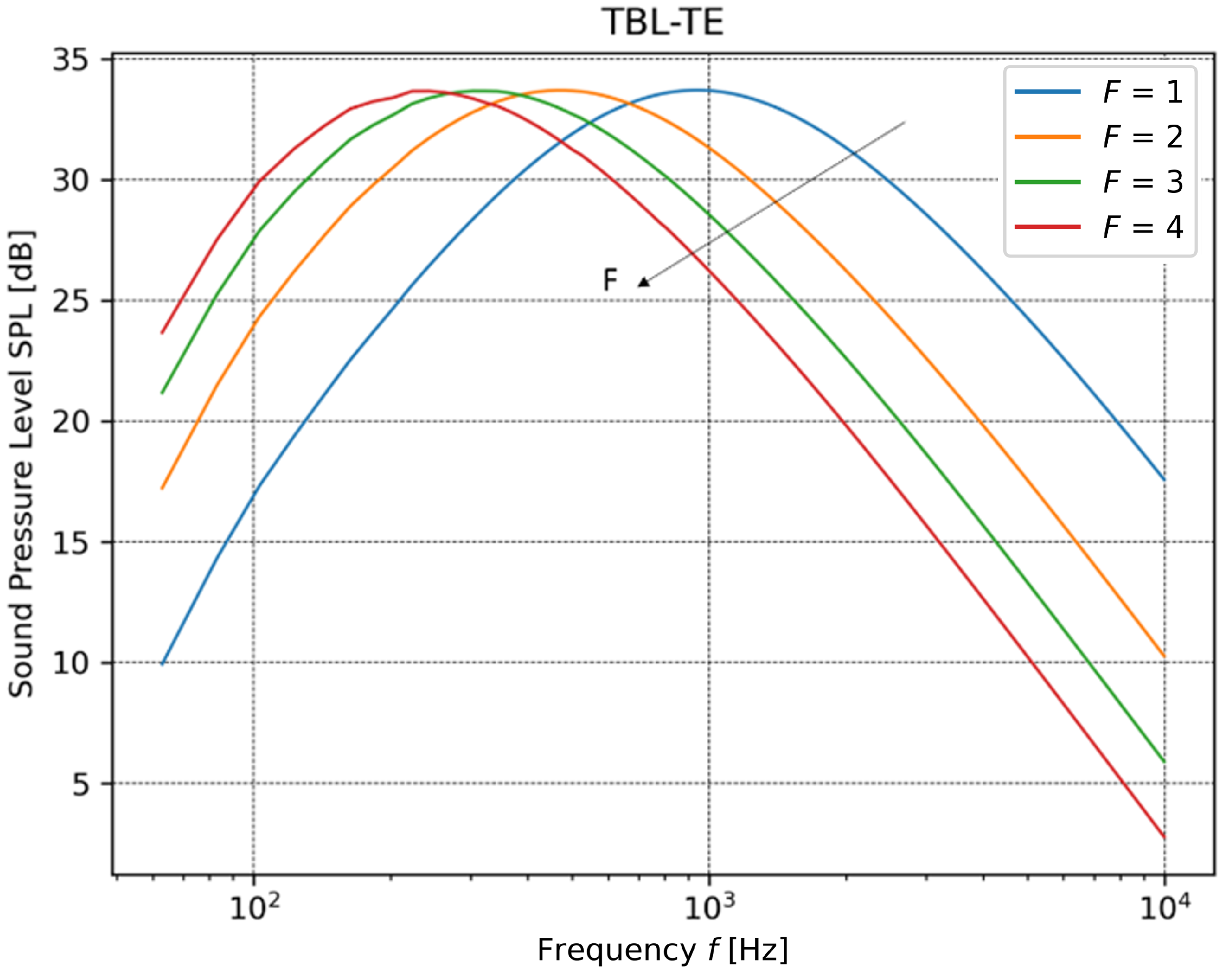
2.2.2. Lowson Model for Turbulent Boundary Layer to Trailing Edge Noise

The interaction between the turbulent boundary layer developed on an airfoil at a high Reynolds number and the trailing edge gives rise to one of the most dominant sources of noise. Based on the work of Brooks, Pope, and Marcolini (BPM) [26], Lowson proposed a formulation in which the airfoil turbulent boundary layer thickness is derived from flat plate theory [34]. The SPL is expressed in one-third octave bands at a given frequency f:

$$\begin{array}{c}\hfill \begin{array}{cc}\hfill & SP{L}_{TE}=10{log}_{10}\left(\frac{\delta M^{5}d}{{r_e}^{2}G\left(f\right)}\right)+128.5\hfill \\ \hfill & G\left(f\right)=\frac{4{\left(\frac{f}{f_p}\right)}^2.5}{\left[{\left(\frac{f}{f_p}\right)}^2\right]};f_p=\frac{0.02U{M}^{-0.6}}{{\delta }^{*}}\hfill \end{array}\end{array}$$

(7)

where the Strouhal peak frequency, $f_p$, the boundary layer thickness, $\delta$, and the boundary layer displacement thickness, ${\delta }^{*}$, are derived from flat plate theory as

$${\delta }^{*}=0.125\delta ·F;\delta =0.37{Re}^{-0.2}.$$

(8)

In Equation (8), F is an empirical correction factor that ranges from 2 to 4 to tune the relationship for real airfoil performance. The F coefficient must be tuned case by case based on the available experimental data of the SPL of the turbine. The overall SPL spectrum reported here is, therefore, computed as the logarithmic sum of both model contributions:

$$SP{L}_{overall}=10{log}_{10}\left({10}^{0.1SP{L}_{Amiet}}+{10}^{0.1SP{L}_{Lowson}}\right).$$

(9)

3. Numerical Methodology

The analysis involved the investigation of two distinct inflow conditions. In the case of ABL simulations, which adopted a constant logarithmic velocity profile, the URANS computations rely on the SST $k-\omega$ turbulence closure. In the TBL-based simulation, the inflow conditions were generated using a precursor channel, and a hybrid delayed-detached eddy simulation (DDES) approach [35] was followed. This modeling combines a URANS formulation-based $k-\omega$ turbulence model in regions close to the ground and an LES formulation in the far field. In so doing, the LES approach resolves the large-scale eddies in the portion of the domain where a sufficient grid refinement is computationally affordable. Both simulations were carried out using OpenFOAM-v21.06. The actuator line modeling is based on the turbinesFoam implementation by Bachant [36]. The aeroacoustic models were implemented by using in-house Python code.

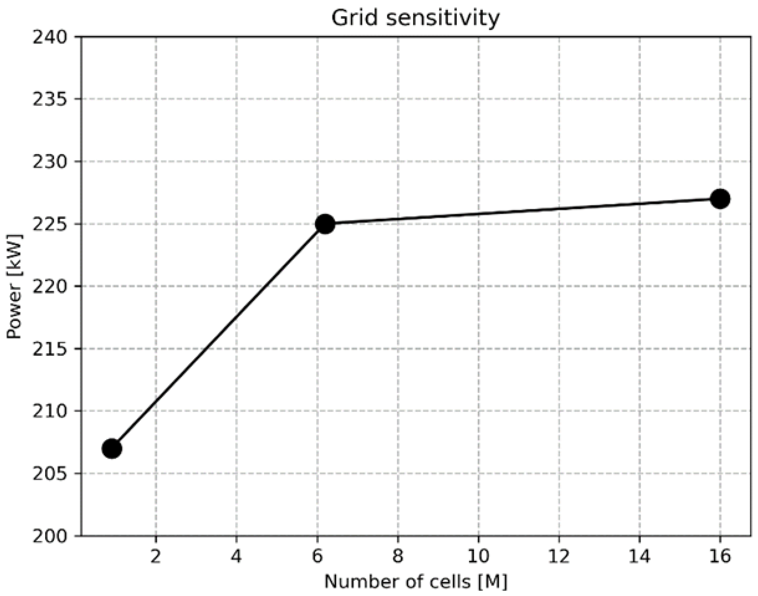
3.1. Computational Domain and Grid

The computational domain was modeled following the sensitivity analysis of Troldborg et al. [37] and is shown in Figure 3. For the generation of time-dependent turbulent inflow conditions, a precursor channel is included in the simulations, with the same cross-section dimensions, that spans 50 diameters (50 × 80 m) in the streamwise direction. The computational grid was generated by using the snappyHexMesh utility. A sensitivity analysis of the grid was carried out using WT power as the convergence parameter. Three grids were generated with rotor zone element sizes of 1.5, 0.75, and 0.375 m, respectively. From Figure 4, the second grid was selected, trading accuracy against computing time. This grid entails 6.1 M cells distributed across four layers of subsequent refinement. The height of the ground cells is 0.922 m. The rotor blades are discretized with 28 elements (1.4 m).

3.2. Boundary Conditions

The atmospheric boundary layer at the inlet of the computational domain is modeled with a logarithmic profile for velocity, turbulent kinetic energy $k_{TKE}$, and specific dissipation rate $\omega$, according to Richards et al. [38] and Yang et al. [39]. For the simulation with full turbulent inflow (TBL), a DDES simulation, including a precursor channel, was run. Periodicity is enforced between the inlet and outlet patches of the precursor domain using OpenFOAM’s built-in arbitrary mesh interfaces (AMI). The outflow from the precursor domain is then employed as the inlet condition for the ALM domain. The ground is treated as a rough wall, with an aerodynamic roughness length of 0.03 m, and wall functions for rough surfaces are applied to the relevant quantities [38]. Slip conditions for velocity are imposed on the upper and lateral boundaries, with convective boundary conditions at the outlet. The pressure condition was set to a zero gradient everywhere except for the outlet patch, where total pressure is imposed.

3.3. Numerical Schemes

Velocity-pressure coupling is based on the PIMPLE algorithm with three inner iterations, with continuity convergence tolerance set to ${10}^{-10}$. A second-order temporal discretization is used in all computations. A time interval is chosen to limit the maximum Courant number to 0.1. The resulting swept angle corresponds to 0.91° of rotor revolution per time step. Upwind schemes are applied to the relevant fields. The convergence threshold is set to ${10}^{-6}$ for all quantities.

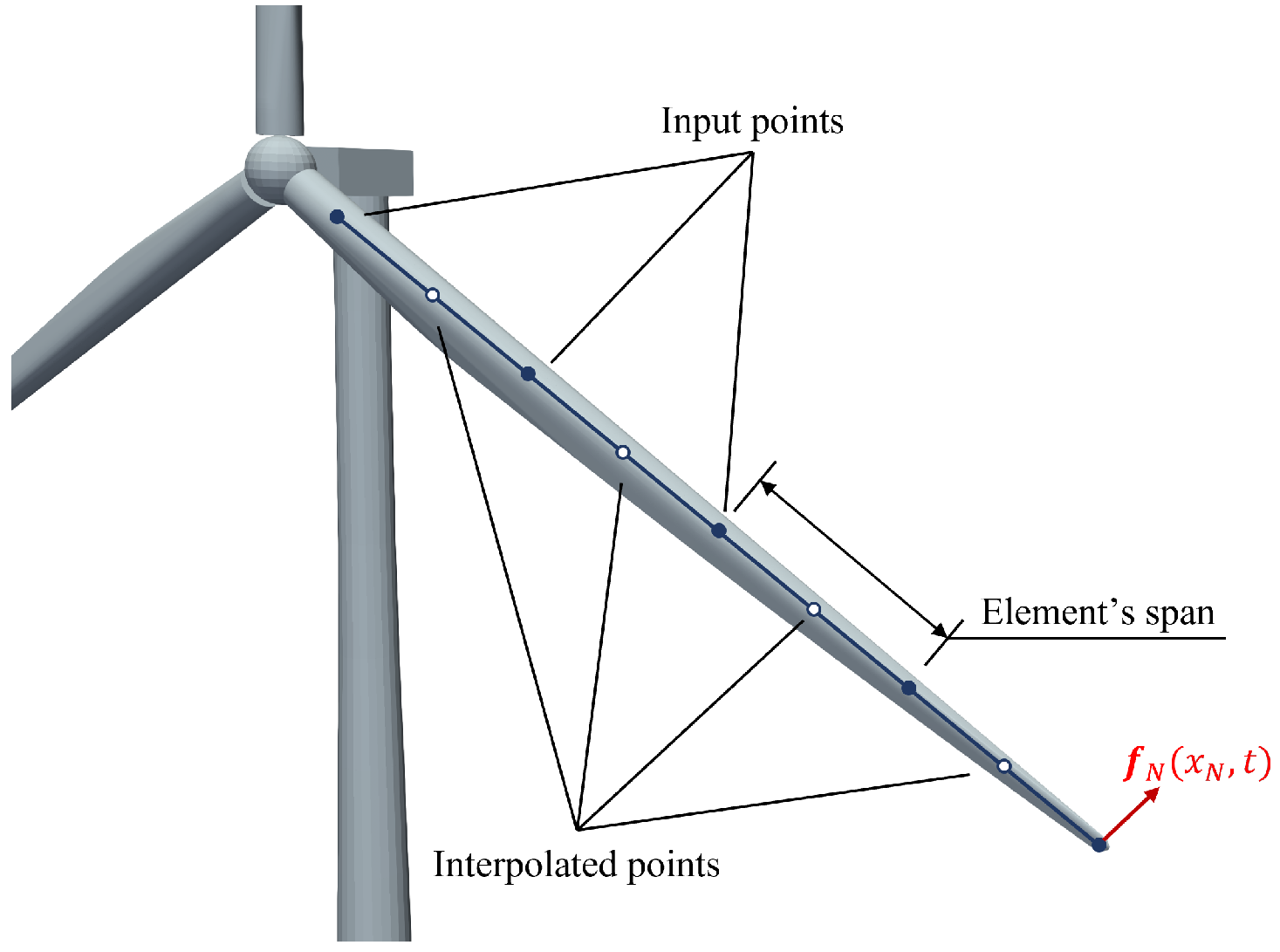
3.4. Aerodynamics and Surrogate Acoustics Coupling

The adopted numerical method is presented in Figure 5. Specifically, the surrogate acoustics algorithm utilizes the fluid dynamic field resolved by the ALM to derive noise predictions. The local relative velocity, incidence, and Reynolds number from the ALM are input into Lowson and Amiet models. Boundary layer thickness, $\delta$, is calculated using X-Foil [40]. The latter exploits the panel method, in which complex surfaces, such as airfoils, are discretized into a set of linear or curved panels. The panel method solves for the pressure and velocity distribution on each panel and then integrates these values to calculate the overall lift, drag, and other aerodynamic characteristics of the geometry. The sensitivity of the method to inflow conditions was investigated by considering two different cases: a stationary inflow with a typical logarithmic atmospheric boundary layer profile (ABL) and a time-dependent inflow derived from a precursor channel for proper turbulence development (TBL).

3.5. Description of the Test Case

The chosen test case is the 2.75 MW Neg Micon NM80/2750, equipped with the LM38.8 blade by Nordex. The geometry and operational data have been obtained from the IEA Wind Task 29 [41]. The turbine is characterized by a rotor diameter, D, of 80 m, a nacelle height of 57.19 m. The rated, cut-in, and cut-off wind velocities are 16, 4.5, and 25.0 m/s, respectively.

4. Validation of the Actuator Line Setup

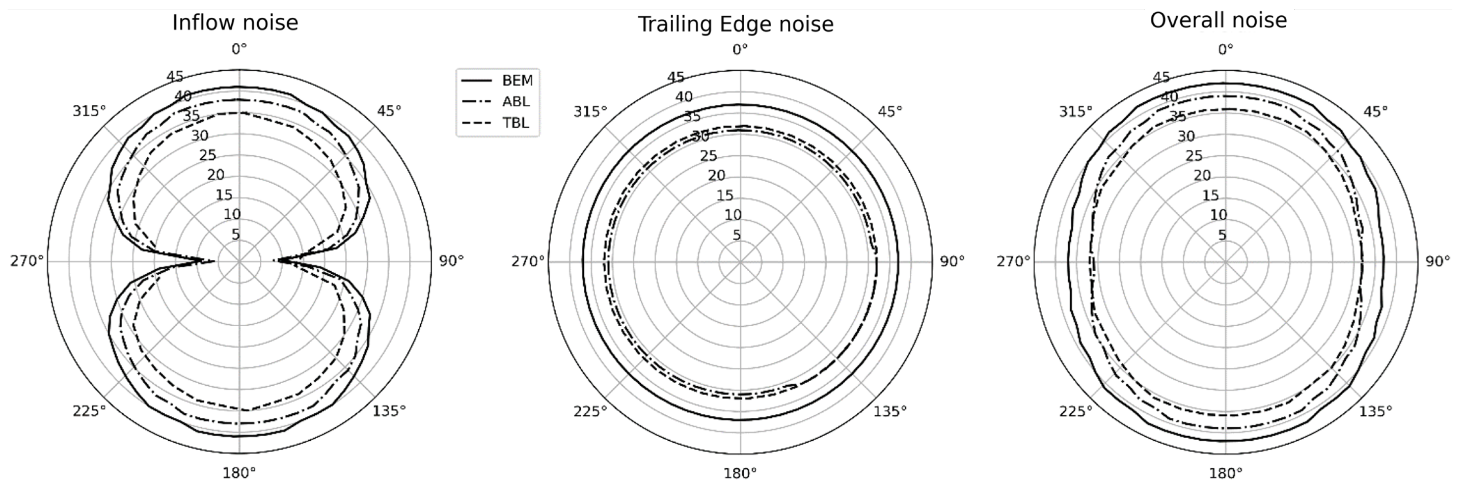
In order to validate the ALM setup, five simulations were carried out under constant inflow conditions, using the atmospheric boundary layer velocity profile, zero yaw angle, and accounting for the pitch-to-feather control system. The simulations were run with free-stream wind velocities of 5, 6.1, 9, 13, and 17 m/s at the hub. Figure 6 presents a comparison between the NM80 rated power and the averaged power from the computations, indicating good agreement. In addition, the turbulent boundary-layer inflow simulation was carried out for the rated wind velocity of 6.1 m/s. In the TBL case, the identical actuator line setup to that of the ABL simulations was employed. Therefore, for the TBL case, additional validation across varying free-stream velocities was not undertaken. The power computed for the turbulent boundary layer case was time-averaged over three rotor revolutions.

In the standard blade element momentum (BEM) theory, the boundary layer thickness, $\delta$, can be computed by treating the airfoil as a flat plate. The accuracy of this method has, however, been the object of discussion by many authors [22,24]. In this work, an empirical multiplicative correction factor, F, is introduced, with a value ranging from 1 to 4. The parameter must be tuned according to reference data. In the test case, the peak frequency scales linearly with F from 1 kHz for $F=1$ to 230 Hz for $F=4$, as reported in Figure 7. The maximum SPL is independent of the choice of F (34.7 dB).

The data from IEA Task 39 [42] were used to validate the numerical technique. The computed far-field noise spectra in the frequency range between 63 and 10,000 Hz are shown in Figure 8, including the results from several open-source and commercial codes from IEA Task 39 [43]. The receiver position was set at the nacelle height and 100 m downstream of the rotor, as prescribed in IEA Task 39. The first attempt at SPL prediction was conducted using BEM theory through an a priori approach, calculating the Reynolds number, angle of attack, and boundary layer thickness based on theoretical computation. According to IEA Task 39, the turbulent intensity and the length scales in the BEM computations were set to 8.96% and 39 m, respectively. The BEM results are perfectly in trend with the other codes, even if a 5 dB higher SPL is observed at all frequencies. The BEM peak frequency is found at 127 Hz, with a maximum SPL of 47 dB, which overpredicts the low-frequency SPL compared to the other codes. The computed spectra using the ALM with both inflow conditions are also included in Figure 8. In these cases, the computed length scales and turbulence intensities are derived from the flow field and not computed a priori. The maximum SPL is found at 37.6 and 39 dB for TBL and ABL, respectively, with both models showing a peak frequency of around 320 Hz.

5. Results

This section reports the comparison between the two different inflows for the wind velocity of 6.1 m/s. Figure 9 shows the instantaneous turbine power as a function of time. The results are in line with the averaged values reported in Figure 6. The TBL shows better agreement with the rated power, whereas the ABL inflow underpredicts the rated power by approximately 30 kW. In the ABL model, the interaction between the blades and the WT tower is evident, with a loss of 2 kW in three negative peaks per rotor revolution, corresponding to the blade passing frequency. This effect is dampened in the TBL model, which, instead, shows a higher variability in terms of turbine power due to the interaction of the blades with the inflow turbulent structures.

Figure 10 displays the computed SPL as a function of the azimuthal co-ordinate of the blade at 200 Hz, which corresponds to the Strohual peak frequency. The inflow noise shows the typical distribution of a dipole source, depending on the directivity term $\overline{D}$. The three models show a reduction in the inflow noise for a blade position corresponding to 90° and 270°, where the blade is parallel to the ground. The lowest maximum value of the SPL is 35 dB from the TBL case, while the simple BEM approach shows an overprediction at the peak frequency, reaching up to 42 dB. Instead, the trailing edge noise shows good agreement between the ABL and TBL simulations and has a mild dependency on the blade azimuthal co-ordinate. The computed trailing edge SPL is in the range of 31.3, 32.1, and 36.9 dB for TBL, ABL, and BEM, respectively. The computed overall SPL reflects the trend already seen in Figure 8, with the highest values found in the BEM a priori computations. The highest SPL corresponds to the blade at 0° and 180°, with the blade orthogonal to the ground. The causes of the differences among the different approaches can be investigated by further analyzing the derivation of the different parameters in Equations (1) and (7).

A comparison of different sections, computed for the vertical blade position, is shown in

Table 1. Computed Reynolds number, inflow flow angle, boundary layer displacement thickness, and boundary layer thickness for the different inflow models at 34, 50, 77, and 99% of the blade span.

Blade Span [%]	BEM				ABL				TBL (Median)
	$\mathit{Re}$ [$\times {\mathbf{10}}^{\mathbf{6}}$]	$\mathit{\alpha }$ [°]	${\mathit{\delta }}^{\mathbf{*}}$ [mm]	$\mathit{\delta }$ [mm]	$\mathit{Re}$ [$\times {\mathbf{10}}^{\mathbf{6}}$]	$\mathit{\alpha }$ [°]	${\mathit{\delta }}^{\mathbf{*}}$ [mm]	$\mathit{\delta }$ [mm]	$\mathit{Re}$ [$\times {\mathbf{10}}^{\mathbf{6}}$]	$\mathit{\alpha }$ [°]	${\mathit{\delta }}^{\mathbf{*}}$ [mm]	$\mathit{\delta }$ [mm]
34	3.83	14.7	27.9	55.9	3.88	15.03	0.71	3.1	3.3	20.82	1.22	4.6
50	4.5	7.59	21.1	43.3	4.41	8.15	0.475	2	4.45	8.87	0.5	2.17
77	4.61	4.3	14.5	29.1	4.52	4.77	0.32	0.5	4.53	5.33	0.31	0.54
99	13.6	8.11	4.3	8.7	11.1	8.25	0.625	2.2	11.1	7.95	0.59	2.0

. The local Reynolds number, defined using the local inflow velocity and section chord, is consistent among the different approaches, although the BEM approach tends to overestimate it, reaching 13.6 M at the blade tip due to the assumption of uniform inflow velocity. A similar trend is found in the computation of the absolute inflow angle $\alpha$. The largest differences are found in the boundary layer thickness computation. In fact, the coupling of the ALM and X-Foil allows for a much better estimation of the quantities, which have different magnitudes with respect to the flat plate assumption. Throughout the entire blade span, the BEM method exhibits an overestimation of the boundary layer thickness, with the most significant discrepancies found near the hub region.

6. Conclusions

The results of coupling the surrogate acoustics models and actuator line methods are shown in this manuscript. Numerical results obtained from the ALM computations were used as input for the surrogate aeroacoustics models. The framework was applied to a horizontal axis wind turbine, NM80, which was tested following the work conditions of IEA Task 39. The results were then compared with the available data from the reduced-order aeroacoustic solvers collected within the task. The analysis of the sound pressure level revealed several insights. First, the models are strongly dependent on the computation of length scales and turbulence intensity. The correction factor, F, which is included in the blade element momentum approach, is arbitrarily chosen and may, therefore, impair systematic and comparative studies on the same families of wind turbines. Its selection does not change the overall sound pressure level of the turbine, but its variation linearly determines the peak frequency. On the other hand, the acoustic computations based on the actuator line method show better results in terms of the sound pressure level spectrum when compared to the other solvers and involving the use of the BEM approach. In particular, the sound pressure level resulting from the turbulent boundary layer approach obtained from a DDES precursor channel presents good agreement when compared to the other solvers, especially for frequencies higher than 130 Hz. The main source of errors was determined by investigating the different terms that appear in the surrogate models. This analysis highlighted the difference between the incidence angle derived from both ALM methods (ABL and TBL) and the one computed a priori for the BEM approach. This disparity directly affects the computation of the boundary layer thickness. In particular, the computation of the boundary layer thickness in the BEM approach, which uses the flat plate assumption, displays the largest uncertainty and deviates considerably from the more precise estimation provided by the panel methods carried out with X-Foil. The results demonstrate that the coupling between the ALM and surrogate acoustics is not only feasible but also provides more accurate results than the BEM approach. Moreover, this SPL estimation method accounts for complex simulation conditions, including non-uniform and time-varying turbulent conditions, which allows for the study of wind farm interaction noise.

References

1. Buchheit, M.; Vandendriessche, T. A European Strategy for Offshore Renewable Energy; European Parliament: Brussels, Belgium, 2022.
2. Qu, F.; Tsuchiya, A. Perceptions of wind turbine noise and self-reported health in suburban residential areas. Front. Psychol. 2021, 12, 736231. [Google Scholar] [CrossRef]
3. Zhu, W.J.; Shen, W.Z.; Barlas, E.; Bertagnolio, F.; Sørensen, J.N. Wind turbine noise generation and propagation modeling at DTU Wind Energy: A review. Renew. Sustain. Energy Rev. 2018, 88, 133–150. [Google Scholar] [CrossRef]
4. De Girolamo, F.; Tieghi, L.; Delibra, G.; Barnabei, V.F.; Corsini, C. Surrogate modeling of the aeroacoustics of an NM80 wind turbine. In Proceedings of the 15th European Turbomachinery Confeerence, Paper n. ETC2023-182, Budapest, Hungary, 24–28 April 2023; p. 900. Available online: https://www.euroturbo.eu/publications/conference-proceedings-repository/ (accessed on 30 May 2023).
5. Wagner, S.; Bareiss, R.; Guidati, G. Wind Turbine Noise; Springer Science & Business Media: New York, NY, USA, 1996. [Google Scholar]
6. Lowson, M. Applications of aero-acoustics to wind turbine noise prediction and control. In Proceedings of the 31st Aerospace Sciences Meeting, Reno, NV, USA, 11–14 January 1993; p. 135. [Google Scholar]
7. Colonius, T.; Lele, S.K. Computational aeroacoustics: Progress on nonlinear problems of sound generation. Prog. Aerosp. Sci. 2004, 40, 345–416. [Google Scholar] [CrossRef]
8. Hardin, J.C.; Hussaini, M.Y. Computational Aeroacoustics; Springer Science & Business Media: New York, NY, USA, 2012. [Google Scholar]
9. Tieghi, L.; Becker, S.; Corsini, A.; Delibra, G.; Schoder, S.; Czwielong, F. Machine-learning clustering methods applied to detection of noise sources in low-speed axial fan. J. Eng. Gas Turbines Power 2023, 145, 031020. [Google Scholar] [CrossRef]
10. Martinez, L.; Leonardi, S.; Churchfield, M.; Moriarty, P. A comparison of actuator disk and actuator line wind turbine models and best practices for their use. In Proceedings of the 50th AIAA Aerospace Sciences Meeting including the New Horizons Forum and Aerospace Exposition, Nashville, TN, USA, 9–12 January 2012; p. 900. [Google Scholar]
11. Ravensbergen, M.; Mohamed, A.B.; Korobenko, A. The actuator line method for wind turbine modelling applied in a variational multiscale framework. Comput. Fluids 2020, 201, 104465. [Google Scholar] [CrossRef]
12. Ouro, P.; Harrold, M.; Ramirez, L.; Stoesser, T. Prediction of the wake behind a horizontal axis tidal turbine using a LES-ALM. In Recent Advances in CFD for Wind and Tidal Offshore Turbines; Springer: New York, NY, USA, 2019; pp. 25–35. [Google Scholar]
13. Baba-Ahmadi, M.H.; Dong, P. Numerical simulations of wake characteristics of a horizontal axis tidal stream turbine using actuator line model. Renew. Energy 2017, 113, 669–678. [Google Scholar] [CrossRef]
14. Lin, X.F.; Zhang, J.S.; Zhang, Y.Q.; Zhang, J.; Liu, S. Comparison of actuator line method and full rotor geometry simulations of the wake field of a tidal stream turbine. Water 2019, 11, 560. [Google Scholar] [CrossRef]
15. Castorrini, A.; Tieghi, L.; Barnabei, V.; Gentile, S.; Bonfiglioli, A.; Corsini, A.; Rispoli, F. Wake interaction in offshore wind farms with mesoscale derived inflow condition and sea waves. Proc. Iop Conf. Ser. Earth Environ. Sci. 2022, 1073, 012009. [Google Scholar] [CrossRef]
16. Mikkelsen, R.; Sørensen, J.N.; Øye, S.; Troldborg, N. Analysis of power enhancement for a row of wind turbines using the actuator line technique. Proc. Iop Conf. Ser. Earth Environ. Sci. 2007, 75, 012044. [Google Scholar] [CrossRef]
17. Troldborg, N.; Larsen, G.C.; Madsen, H.A.; Hansen, K.S.; Sørensen, J.N.; Mikkelsen, R. Numerical simulations of wake interaction between two wind turbines at various inflow conditions. Wind Energy 2011, 14, 859–876. [Google Scholar] [CrossRef]
18. Breton, S.P.; Shen, W.Z.; Ivanell, S. Validation of the actuator disc and actuator line techniques for yawed rotor flows using the New MEXICO experimental data. Proc. Iop Conf. Ser. Earth Environ. Sci. 2017, 854, 012005. [Google Scholar] [CrossRef]
19. Nilsson, K.; Shen, W.Z.; Sørensen, J.N.; Breton, S.P.; Ivanell, S. Validation of the actuator line method using near wake measurements of the MEXICO rotor. Wind Energy 2015, 18, 499–514. [Google Scholar] [CrossRef]
20. Bhargava, V.; Samala, R. Acoustic emissions from wind turbine blades. J. Aerosp. Technol. Manag. 2019, 11, e4219. [Google Scholar] [CrossRef]
21. Buck, S.; Oerlemans, S.; Palo, S. Experimental validation of a wind turbine turbulent inflow noise prediction code. AIAA J. 2018, 56, 1495–1506. [Google Scholar] [CrossRef]
22. Oerlemans, S.; Schepers, J.G. Prediction of wind turbine noise and validation against experiment. Int. J. Aeroacoust. 2009, 8, 555–584. [Google Scholar] [CrossRef]
23. Barlas, E.; Zhu, W.J.; Shen, W.Z.; Dag, K.O.; Moriarty, P. Consistent modelling of wind turbine noise propagation from source to receiver. J. Acoust. Soc. Am. 2017, 142, 3297–3310. [Google Scholar] [CrossRef]
24. Moriarty, P.; Guidati, G.; Migliore, P. Prediction of turbulent inflow and trailing-edge noise for wind turbines. In Proceedings of the 11th AIAA/CEAS Aeroacoustics Conference, Monterey, CA, USA, 23–25 May 2005; p. 2881. [Google Scholar]
25. Sorensen, J.N.; Shen, W.Z. Numerical modeling of wind turbine wakes. J. Fluids Eng. 2002, 124, 393–399. [Google Scholar] [CrossRef]
26. Brooks, T.F.; Pope, D.S.; Marcolini, M.A. Airfoil Self-Noise and Prediction; Technical Report No. L-16528; CreateSpace Independent Publishing Platform: Scotts Valley, CA, USA, 1989. [Google Scholar]
27. Grosveld, F.W. Prediction of broadband noise from horizontal axis wind turbines. J. Propuls. Power 1985, 1, 292–299. [Google Scholar] [CrossRef]
28. Oerlemans, S. Wind Turbine Noise: Primary Noise Sources; National Aerospace Laboratory NLRL: Amsterdam, The Netherlands, 2011.
29. Moriarty, P.; Migliore, P. Semi-Empirical Aeroacoustic Noise Prediction Code for Wind Turbines; Technical Report No. NREL/TP-500-34478; National Renewable Energy Lab.: Golden, CO, USA, 2003.
30. Amiet, R.K. Acoustic radiation from an airfoil in a turbulent stream. J. Sound Vib. 1975, 41, 407–420. [Google Scholar] [CrossRef]
31. Bortolotti, P.; Branlard, E.; Platt, A.; Moriarty, P.; Sucameli, C.; Bottasso, C.L. Aeroacoustics Noise Model of OpenFAST; Technical Report No. NREL/TP-5000-75731; National Renewable Energy Lab.: Golden, CO, USA, 2020.
32. Guidati, G.; Bareiss, R.; Wagner, S.; Parchen, R.; Guidati, G.; Bareiss, R.; Wagner, S.; Parchen, R. Simulation and measurement of inflow-turbulence noise on airfoils. In Proceedings of the 3rd AIAA/CEAS Aeroacoustics Conference, Atlanta, GA, USA, 12–14 May 1997; p. 1698. [Google Scholar]
33. Moriarty, P. NAFNoise User’s Guide; National Wind Technology Center, National Renewable Energy Laboratory: Golden, CO, USA, 2005.
34. Schlichting, H.; Kestin, J. Boundary Layer Theory; Springer: New York, NY, USA, 1961; Volume 121. [Google Scholar]
35. Strelets, M. Detached eddy simulation of massively separated flows. In Proceedings of the 39th Aerospace Sciences Meeting and Exhibit, Reno, NV, USA, 8–11 January 2001; p. 879. [Google Scholar]
36. Bachant, P.; Goude, A.; Wosnik, M. Zenoodo. Turbinesfoam: v0. 0.7. 2016. Available online: https://zenodo.org/record/49422 (accessed on 31 March 2018).
37. Troldborg, N. APA. Actuator Line Modeling of Wind Turbine Wakes; APA: Washington, DC, USA, 2009. [Google Scholar]
38. Richards, P.; Hoxey, R. Appropriate boundary conditions for computational wind engineering models using the k-ϵ turbulence model. J. Wind. Eng. Ind. Aerodyn. 1993, 46, 145–153. [Google Scholar] [CrossRef]
39. Yang, Y.; Gu, M.; Jin, X. New inflow boundary conditions for modeling the neutral equilibrium atmospheric boundary layer in SST k-ω model. J. Wind Eng. Ind. Aerod 2012, 97, 88–95. [Google Scholar] [CrossRef]
40. Drela, M. XFOIL: An analysis and design system for low Reynolds number airfoils. In Proceedings of the Low Reynolds Number Aerodynamics, Notre Dame, IN, USA, 5–7 June 1989; Springer: New York, NY, USA, 1989; pp. 1–12. [Google Scholar]
41. Schepers, J.; Boorsma, K.; Madsen, H.A.; Pirrung, G.; Bangga, G.; Guma, G.; Lutz, T.; Potentier, T.; Braud, C.; Guilmineau, E.; et al. IEA Wind TCP Task 29, Phase IV: Detailed Aerodynamics of Wind Turbines. 2021. Available online: https://zenodo.org/record/4813068 (accessed on 26 May 2021).
42. Bertagnolio, F.; Dtu, A.F.; Seel, F.; Lutz, T.; Iag, C.H.; Balterria, G.U.; Boorsma, K.; Appel, C.; Bortolotti, P. IEA Wind TCP-Task 29 T3. 7 & Task 39 Wind Turbine Noise Code Benchmark-Preliminary Results. 2021. Available online: https://iea-wind.org/wp-content/uploads/2021/05/report_WTNCBenchmark.pdf (accessed on 24 February 2021).
43. Casalino, D.; van der Velden, W.C.; Romani, G. A framework for multi-fidelity wind-turbine aeroacoustic simulations. In Proceedings of the 28th AIAA/CEAS Aeroacoustics 2022 Conference, Southampton, UK, 14–17 June 2022; p. 2892. [Google Scholar]
Figure 1. Actuator line scheme: N is the number of elements, x N are position vectors, and f N are aerodynamic forces.
Ijtpp 08 00043 g001
Figure 2. Scheme of directivity angles.
Ijtpp 08 00043 g002
Figure 3. Computational domain and grid refinements.
Ijtpp 08 00043 g003
Figure 4. Grid sensitivity analysis based on a power comparison between grids with different rotor cell refinement.
Ijtpp 08 00043 g004
Figure 5. Scheme of surrogate acoustics and actuator line coupling methodology.
Ijtpp 08 00043 g005
Figure 6. Comparison between the rated power and the computations: ABL inflow (red circles) and TBL inflow (green diamond).
Ijtpp 08 00043 g006
Figure 7. Sensitivity of the Lowson model as a function of the correction factor F.
Ijtpp 08 00043 g007
Figure 8. Comparison of the SPL spectra derived from the surrogate acoustic solver by IEA Task 39 participants (dashed-dotted lines) and the SPL spectra obtained from the current implementation of surrogate acoustic models (markers).
Ijtpp 08 00043 g008
Figure 9. WT power as a function of rotor revolutions; TBL (dashed-dotted) and ABL (solid line).
Ijtpp 08 00043 g009
Figure 10. The SPL from a single blade is plotted as a function of the azimuthal co-ordinate of the blade for the various models and cases. The receiver is placed at nacelle height, 100 m downstream.
Ijtpp 08 00043 g010