1. Introduction
The design of compressor blades today is heavily supported by optimizers, CFD solvers, and other types of numerical methods. The rapid development of improved algorithms and raw computational power has allowed designers to produce ever-improving blade designs with these new methodologies. However, they do rely on the accuracy of the solver for the desired design purpose. CFD-RANS solvers for example are typically considered to have an adequate level of accuracy for most design applications, even if they sometimes fall short in detail. However, this is not as trivial in transonic flow conditions due to the complex modeling challenges they present for any such solver. The presence of an inherently unsteady shock structure that impacts the entire flow field, its potential strong interaction with the boundary layer, and cascade-specific operating conditions, such as choking at unique incidences [
1], are just some of the possible sources of significant discrepancies that (U)RANS users need to be aware of. In practice, designers are forced to apply undesirably high design margins, as explained in recent work [
2].
In order to help address these shortcomings, it is imperative to support the numerical methods with experimental data. For this purpose, linear cascade wind tunnels present themselves as ideal facilities due to the clean flow conditions and optical access they are able to achieve when compared to rotating compressor rigs. Nevertheless, operating these facilities is still a complex task, as summarized in reference [
3]. Because of this, it is still rare to have the opportunity to validate a new design for these applications experimentally (perhaps more today than ever before). In the past, research institutions and organizations like ONERA [
4] and General Motors [
5] have designed and operated linear cascade wind tunnels for high-speed flow applications. Today, on the other hand, research projects that advance the fundamental understanding of these types of flows reside in the facilities of just a few research institutions, such as the IMP PAN’s Transonic Wind Tunnel [
6] and the DLR’s own Transonic Cascade Wind Tunnel (TGK) in Cologne [
7].
The TGK is a leading-edge, continuous-loop linear cascade wind tunnel that has been operating in Cologne for over 40 years [
8]. The wind tunnel can be operated at Mach numbers between 0.2 and 1.4, while achieving Reynolds numbers between
and
. The configuration of the wind tunnel has been continuously developed to allow the investigation of an increasing number of transonic cascade designs at different operating points of interest. These features include suction devices around the test section, modifiable wall positions and outlet cross-section during operation, and a configurable cascade angle with respect to the horizontal axis among others. This means that an experienced user can control the flow conditions at the inlet, the flow periodicity, the outlet back pressure, the size of the sidewall boundary layers, and other conditions that are important to find the desired operating point of any given design. These characteristics make it a unique facility in the world and ideal for investigating transonic flow applications of this nature.
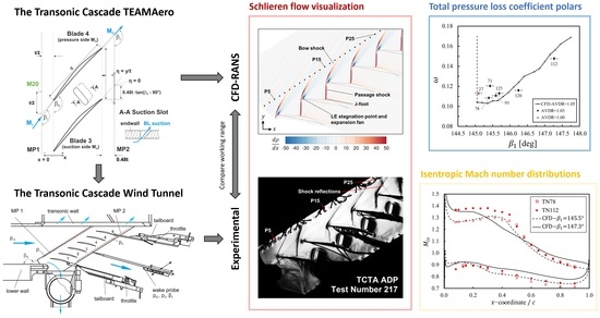
This publication focuses on assessing the most relevant discrepancies that exist between numerical and experimental research within the context of compressor blade designs [
9]. The paper begins by presenting the Transonic Cascade TEAMAero (TCTA), which is a recent product of the author’s work, employing in-house state-of-the-art design techniques. This cascade was designed within the context of the H2020 research consortium, TEAMAero, dedicated to the study of shock–boundary layer interactions and mitigation strategies in transonic flow applications. The TGK facility previously mentioned is then described in detail, along with the steady measurement techniques employed for this study. The results obtained enable a direct comparison between the output of the design process and the actual working range performance of the TCTA for discussion. The experimental investigation of this cascade then presents a unique opportunity to validate the numerical procedures, but also to identify its shortcomings that are yet to be addressed.
2. The Transonic Cascade TEAMAero
The TCTA is a compressor cascade based on the design of Member 1532 in [
10,
11]. The original design was obtained from an optimization procedure employing the optimization suite, AutoOpti, and supported by the CFD-RANS solver, TRACE [
12,
13]. This section provides an overview of the original optimization process before describing the difference with the final TCTA design and presenting its configuration in the wind tunnel.
2.1. Design Process Overview
The process chain of the original optimization consisted of three main procedures: generating a new cascade geometry, meshing the cascade, and estimating its performance through RANS simulations. The simulations were performed applying the
k-
SST RANS model coupled with the
transition model [
14,
15]. The result from this process chain was managed through AutoOpti, which was set to minimize two objectives: the flow losses at the aerodynamic design point (ADP), and over the working range (WR) at a constant inlet Mach number (M
). These flow losses were quantified by the total pressure loss coefficient (
). The ADP of the cascade was defined based on a reference cascade in terms of the inflow angle (
1) and aerodynamic loading measured by the de Haller number =
(DH). The optimization result yielded several candidate designs, from which, Member 1532 was selected as the basis of the final TCTA design. For further details, the reader may refer to the original publication.
From the basis provided by Member 1532, two small modifications were made to the original design: the ratio between the leading edge length and radius was increased, and the cascade pitch was reduced. The first modification provides a more elongated and rounded leading edge, which facilitates its manufacturing and may slightly alleviate the strong gradients experienced near the leading edge based on previous experience. The second modification decreases the mass flow load of the wind tunnel, which was necessary after detailed load estimates were performed. These parameters were both modified within the constraints of the original optimization to ensure that the new design was still representative of the design process followed. The main design parameters of the final TCTA cascade for the experimental campaign are then presented in
Table 1.
2.2. Wind Tunnel Configuration
The TCTA cascade is shown in
Figure 1 along with its configuration when installed in the TGK. Six blades were prepared for this experimental campaign, and were manufactured from low-alloy steel, with a mean surface roughness value (
) that was maintained below 0.8 µm. The cascade is mounted on two plexiglass sidewalls that allow good optical access to the flow during the experiments. The sidewalls count with suction slots for the five cascade passages located at 80% of the chord length of the adjacent lower blade. The suction through the slots can be controlled and helps impose the size of the sidewall boundary layer through the passage and, therefore, the axial velocity density ratio (AVDR). This parameter will be further described in the following sections. The designs of the slots are shown in
Figure 1b and are based on previous experiences. This figure also shows the definition of the inlet and outlet measurement planes, MP1 and MP2, respectively. The sidewalls in turn are mounted on a circular section of the wind tunnel that can be rotated to a precise angle with respect to the horizontal or cascade angle (
). This angle was varied between 144.9° and 147.8° throughout the duration of the test campaign.
Figure 1b also shows the top and bottom suction devices, the lower wall, the outlet tailboards, their throttles, and the lower tailboard hinge. All of these devices can be adjusted separately during the experiment to configure the wind tunnel for the desired operating point.
3. Numerical Methods
The numerical setup employed for the CFD simulations in this study was taken, for the most part, from the design process presented in
Section 2 and is reviewed in this section in detail before presenting the estimated performance of the TCTA.
3.1. Numerical Setup Overview
As previously mentioned in
Section 2.1,
TRACE’s RANS solver is employed with the 2003 version of Menter’s
k-
SST turbulence model and the
transition model. This is considered throughout the paper to be the main numerical setup or configuration. The transition model is important given that the TGK features a low turbulence level in the order of
[
16], which means that the typical flow topology observed for transonic cascades is the laminar flow up to the passage shock foot, under which a laminar separation bubble forms that triggers the transition to turbulent flow. This flow topology is captured well with this solver configuration based on the previous design process followed. In addition to this configuration, a new alternative setup was also employed, which applied the DLR-developed SSG/LRR-
full Reynolds stress model (RSM) with the same
transition model mentioned [
17]. The RSM model helps provide a point of comparison with respect to the main configuration for operating points with high inflow angles and significant flow separation, which could be more appropriate for the RSM model. The application of the same transition model in
TRACE also helps provide a direct comparison between the models for this application. Unless otherwise specified, the CFD results presented in this paper were obtained with the main configuration.
The domain is a quasi-3D setup with periodic boundaries in the pitch direction, and an inlet and outlet defined at approximately two axial chord lengths upstream and downstream of the leading and trailing edges. The inlet and outlet apply the non-reflecting boundary conditions presented in [
18]. The operating point is defined by prescribing the total pressure and temperature at the inlet, along with the static pressure at the outlet. The inlet Mach number is then a result of the simulation. The simulated blade span has a length of 5% of the chord and is defined with a symmetry condition at the blade hub and an inviscid contracting wall at the blade tip. The contracting wall helped impose the AVDR in the simulation. This parameter describes the flow area contraction amount at the outlet compared to the inlet due to the sidewall boundary layer, as defined in [
19]. This parameter is important to define the operation of the cascade because a large sidewall boundary layer—or high AVDR—causes the passage shock to shift forward, and accelerates the subsonic flow downstream of the shock. This generally aids the reattachment of the flow and reduces the losses at the outlet but at the cost of an earlier onset of choke.
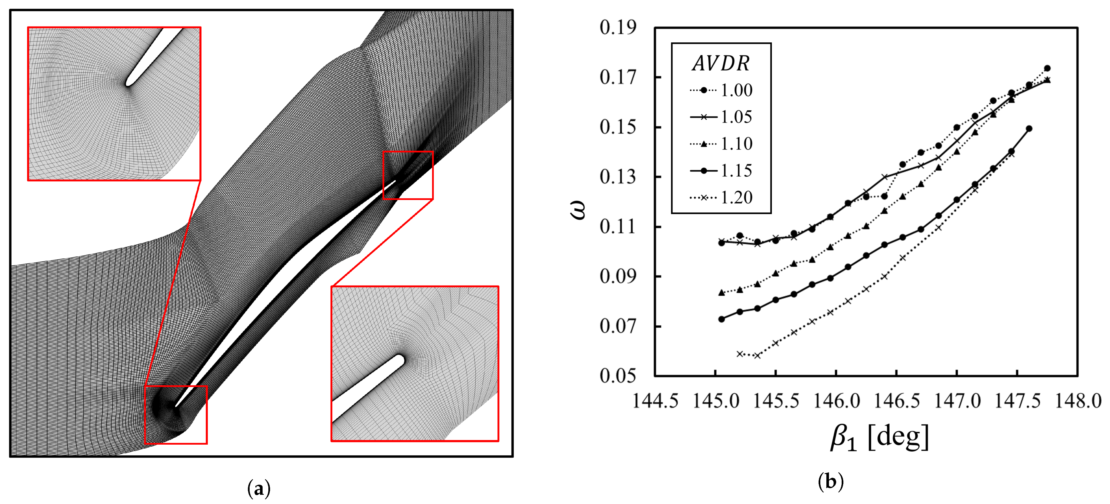
Lastly, the mesh is taken directly from the previous optimization design process and is shown in
Figure 2a. It consists of a multi-block structured mesh with a total of 65,000 faces in the blade-to-blade view and 7 equidistant points in the span-wise direction. This amounts to approximately 400,000 elements. The convergence procedure by [
20] was followed, resulting in a mesh with a grid convergence index of 1%; this balance proved to be a good compromise between accuracy and computation length. For more details on the convergence and mesh validation procedure followed, the reader is referred to [
11].
3.2. Estimated Cascade Performance
The performance of the new TCTA design was then re-evaluated with the main numerical configuration described, as shown in
Figure 2b. The working range of the cascade is shown in terms of total pressure loss coefficient polars at a constant inflow Mach number of 1.2 and different AVDR values. Even though the cascade was optimized for an AVDR of 1.20; this parameter is notoriously difficult to match experimentally because it depends strongly on the inflow angle, which cannot be measured in real time. Additionally, the wind tunnel favors low AVDR values due to its low level of turbulence. For these reasons, the cascade performance was evaluated for AVDR values from 1.20 down to 1.00 to guide the configuration of the wind tunnel as the operating conditions were explored.
It must be restated in this paper that the lowest inflow angle shown in
Figure 2b for every AVDR line corresponds to the lowest angle resolved by the CFD solver at the desired inflow Mach number. This was then considered to be the numerical onset of cascade choke, where the losses continue to increase at unique incidence conditions. However, it is difficult to explicitly solve this section of the graph based on the boundary conditions previously described. Finally, as observed in the original optimization, many of the simulations evaluated converged with some level of periodic numerical oscillations in the domain. In [
11], it was discussed that this most likely occurs due to the highly unsteady nature of the flow in these conditions, especially at higher inflow angles with large areas of separated flow. When this was the case, the solution was averaged over two cycles of the numerical instability according to the mass flow at the outlet, as done for the optimization.
4. Experimental Methods
In order to validate the estimated performance, the TCTA was tested at the TGK wind tunnel. This section begins with a description of the flow measurement techniques employed, followed by an explanation of the procedure followed to estimate the performance and its related measurement error, and a word on the limitations and sources of errors of the experimental methods applied.
4.1. Flow Measurement Techniques
Several techniques were employed in order to measure the flow parameters of interest, including the total pressure, total temperature, static pressure, and flow angle. The rest of the flow conditions reported in this paper were derived from these measurements. The total pressure and total temperature of the incoming flow are taken in the settling chamber of the wind tunnel. The flow is assumed to be adiabatic so that the total temperature remains constant throughout. At the inlet, the cascade sidewalls are instrumented with 29 pressure taps at the MP1 shown in
Figure 1a. These are evenly spaced out to maintain five taps per pitch. The blades themselves are also instrumented with pressure taps along the midspan. All the blades have one tap on the suction surface at 10% of the chord to track the periodicity of the flow in the different passages. The third and fourth blades are additionally instrumented with 17 and 12 taps along the suction and pressure surfaces, respectively. Finally, the flow at the outlet is measured with a three-hole probe positioned at the blade midspan, as shown in
Figure 1b. The probe can be moved parallel to the cascade along the MP2 outlet plane in
Figure 1a.
In order to measure the flow angle over the MP1, the unobtrusive laser-2-focus (L2F) anemometry technique is used from [
21]. This device directs two distinct laser beams of high intensity inside the test section. The distance and orientation between the laser beams is known, so that the velocity magnitude and angle of a particle going through the two beams can be estimated with high precision. In order to achieve this, the laser beams are rotated 360° at every measurement point in order to obtain a distribution of the particles observed at different angles. This technique allows the measurement of the flow angle with an error margin of
, and can also provide the flow angle before and after a shock. For measurements made with this technique, 2 pitch lengths were covered along the MP1 with 10 points per pitch, and starting from the midpoint between the second and third blades, the 20th measurement point is shown in
Figure 1a with the label M20 for reference.
Finally, a Schlieren setup was employed, consisting of an LED light source redirected through the test section with the help of two large concave mirrors. The resulting image was captured with a CMOS camera at 21 frames per second and covers a 321 × 270 mm area with a density of 7.6 pixels/mm in either direction. This visualization was important throughout the tests in order to quickly assess the shock structure and modify the configuration of the wind tunnel if necessary, for instance, to improve the flow periodicity. A picture of the cascade in the wind tunnel is shown in
Figure 3.
4.2. Overall Performance Derivation and Measurement Error
In order to report on the overall performance of the cascade, the measurements at the outlet are processed based on the procedure outlined in [
3] for the parameters typically measured in this type of experimental campaign. Namely, the flow is first averaged to an equivalent uniform flow based on the conservation principles of mass, momentum, and energy. This is done assuming a 2D, isentropic, and adiabatic flow developing far downstream of the cascade. The flow conditions calculated are then used to determine the performance parameters of interest, including the AVDR,
, flow turning (FT), and others. In terms of measurement error, the pressure-based measurements have a low percentage error of 0.02%, with respect to the full measurement scale. Additionally, the error on the angle measurements from the L2F at the inlet and the probe at the outlet is estimated to have an absolute error of 0.1°. However, these error margins propagate for the calculation of the averaged flow parameters previously explained. The total pressure loss coefficient of the cascade reported in this paper has an estimated measurement error of 1%.
4.3. Limitations of the Experimental Configuration
The main difficulty throughout this experimental campaign was related to the fact that the measurement techniques employed for this study are not time-resolved and measured only the steady properties of the flow over the cascade. This was complicated because a high level of unsteadiness was expected during the tests from previous experiences at the TGK [
7]. The type of unsteadiness observed in these configurations emerges from the strong shock–boundary layer interaction (SBLI) that occurs between the passage shock and the boundary layer on the suction surface of the blade. This behavior has been observed from as early as 1938 [
22]. Since then, it has been reproduced and studied experimentally with different wind tunnel configurations and numerically with high-fidelity solvers, such as in [
23].
The TCTA was no exception, with the passage shock oscillating at an amplitude of roughly 10% of the blade chord. This is a notable source of uncertainty for the different measurements, starting with the L2F inflow angle measurements because of the related movement of the bow shocks and the fact that the measurements must be taken over an extended period of time. The situation may arise where the same shock is observed two or more times, as shown in
Figure 3b. Even though results with this level of unsteadiness were discarded, the measurements kept were still averaged over one pitch starting from the first point after the shock. In order to further minimize these uncertainties, the measurements were kept only if the flow was considered sufficiently stable and periodic, if the L2F measurements were comparable to each other, and if the angle measured was consistent with the magnitude of the M
near the leading edge of the middle passage. These conditions were best met with the cascade operating at an AVDR of 1.05, which will be the focus for the remainder of the paper.
Additionally, a periodic flow is difficult to achieve in linear cascade configurations, as thoroughly explained in [
3]. Regardless of the extensively modifiable configuration of the TGK, the flow is inevitably affected by asymmetrical conditions as it travels through a different number of bow shocks and their reflections into any given passage. Nevertheless, care was taken to set up the middle passages with the most periodic conditions possible. This has been defined at the TGK as a total pressure delta below one kPa between the first and last measurements of a traversal with the three-hole probe across the third blade. A broad traversal is also carried out before these measurements to ensure that the peak total pressure loss across blades two to four is comparable. This is coupled with the inspection of the shock structure, as revealed by Schlieren visualization, and an examination of the isentropic Mach number, as measured by the pressure tap at the 10% chord point of all the blades.
Finally, the last source of uncertainty relates to the effects the unsteady flow might have on the measured steady performance. This is especially relevant when comparing these results to CFD-(U)RANS simulations that have been shown to not capture the nature and extent of these effects for the given application [
2]. This discrepancy is recognized, though the comparison is performed because RANS remains the automatic choice for design purposes, as done for the design of the TCTA. This comparison will then hopefully inform the limitations of the current design processes with respect to an actual end design. It may also guide future research aimed at developing these methods for the purpose of capturing these effects if they are relevant to any given application.
5. Results and Discussion
Over the course of the campaign, 126 operating points were measured with outlet probe traverses and blade isentropic Mach number (M
) distributions. These measurements helped locate the operating points of interest based on a rough estimate of the inflow angle derived from the cascade angle,
. If the measurements seemed to indicate a point of interest, new tests were performed with L2F to determine the actual angle. In the end, 20 measurements were made with L2F, over which the cascade was observed to operate at different AVDR conditions between 1.00 and 1.15, with the best results obtained at 1.05. Even though the optimization’s AVDR was not precisely matched, the results still helped validate the design process based on the understanding of the AVDR discussed in
Section 3.1. The results are presented in three parts, starting with the estimated working range of the cascade, and moving on with more detailed comparisons of the design inflow angle and other points of interest.
5.1. The Working Range of the TCTA
The working range was determined with six operating points, corresponding to TNs 71, 78, 93, 112, 125, and 126. These points cover the different regions of interest for the cascade’s working range at an AVDR of 1.05: two points in choked conditions (TN 71, 78), two points near the design inflow angle (TN 93, 125), and two points with high inflow angle (TN 112, 126). These points are first shown in
Figure 4 in terms of the L2F angle distribution over the pitch, and then in terms of the total pressure loss coefficient polar. In this figure, an additional point is shown for comparison, TN 27, with an AVDR of 1.00 and operating in choked flow conditions. Finally, the estimated RANS performance at an AVDR of 1.05 is also included in the polar, with the assumed choke line, in order to facilitate the comparison with the test points.
In
Figure 4a, it is shown that most of the L2F measurements have comparable characteristics in terms of inlet angle distributions. More specifically, the measurements from TN 71, 78, 93, 125, and 126 are shown to have the main bow shock located at M8. These measurements are also shown to have similar passage lengths of up to M20 or M21 before the next bow shock is observed. They also show a progressively higher
magnitude throughout the distribution, allowing a direct comparison of the cascade performance between them. Only TN 112 shows some differences in the
distribution, given that it is operating at a considerably higher inlet angle and the bow shocks accordingly have a much steeper angle with respect to the cascade’s MP1. For this case, the angle has been averaged between measurement positions M12 and M20. Finally, the distribution of TN 27 also shows a small shift in the opposite direction, which can be attributed to the lower AVDR in the passage.
The estimated
angle is then used to locate the operating points in the cascade’s
-polar, shown in
Figure 4b. Specific details of the inflow conditions for each test are also presented in
Table 2. The comparison in
Figure 4b shows a satisfactory agreement of the cascade’s performance over the working range. Even though the losses do not precisely meet the CFD curve, they lie within a percentage error of 3–6% across the entire working range. The differences observed in the loss values can also be partially explained by the difficulty of matching the exact AVDR value. Points such as TN 112 and 126 were estimated to have a slightly higher AVDR, which would be expected to produce lower losses. This is also consistent with the measurements of TN 78, 93, and 125, with slightly lower AVDR values. Even with these small discrepancies, the cascade was validated to have a wide range of operations (
), with notably low losses (
), and high aerodynamic loading (
), as per the objectives of the original optimization.
However, one sensitive difference must be noted on the inflow angle for choked operating conditions. As shown in
Figure 4b, this condition was found to be at inflow angles of 145.1° and 145.4° for AVDRs of 1.00 and 1.05, respectively. This reduction of the working range at a higher AVDR is expected due to the lower effective passage area. However, this effect is barely captured in the RANS simulations up to an AVDR of 1.20, as shown in
Figure 2. This is a clear limitation of the numerical setup that would need to be addressed if the positions of the ADP and the choke angle were of higher importance. Possible sources of discrepancy could be related to the inability of the solver to explicitly resolve the flow in a unique incidence condition, or to the modeling of the domain itself with a quasi-3D domain and contracting inviscid walls.
5.2. Detailed Comparison at the ADP Inflow Angle
The results from the point closest to the inflow design angle, TN 125, are now shown in detail in
Figure 5. This figure shows the M
distribution over the blade, as well as the loss and angle measurements in the outlet along the
-axis previously defined in
Figure 1a. In this figure, and focusing on the suction surface line, the M
distribution is shown to generally match very well with the CFD results. The front part of the distribution, which at constant M
depends strongly on
, is shown to lie in between the CFD curves to validate the
L2F measurement of
. Additionally, the rear part of the distribution also follows the CFD curve very well, which depends strongly on the AVDR. The main difference is observed near the shock position at a 30% chord length, where there are strong unsteady effects, and a laminar separation bubble is observed until the 45% mark. Even though flow transition is also triggered under the shock in the simulations, the actual size of the separation bubble and its effect on the distribution are barely captured. Some differences can also be noted in the pressure surface distribution, but this is to be expected given that it is heavily influenced by the flow on the suction surface of the adjacent passage.
The shortcomings of RANS solvers become much more evident in
Figure 5b. The wake is shown to actually be much wider and to have a lower maximum value in the experiments than in the simulations. These results suggest that the diffusion characteristics of the flow as it develops behind the cascade are not fully captured in the RANS simulations. This may be partially or solely due to the missing influence of the unsteady shock–boundary layer interaction previously discussed. Significant differences are also observed in the outlet flow angle distribution, where the simulations this time show a much more attenuated variation of the flow angle. Even though the experiments show some level of non-periodicity, as shown in the angle distribution with measurements starting at 136.7° and finishing at 135°, it is clear that this does not account for the differences observed. Overall, the RANS results seem to provide sufficiently good results to measure the general performance of the cascade, as shown in
Figure 4. This was also the case with the de Haller number (not shown), which was consistently predicted within a 3% margin over the working range. Nevertheless, care must be taken when using it to estimate specific characteristics of the flow, especially across the wake region.
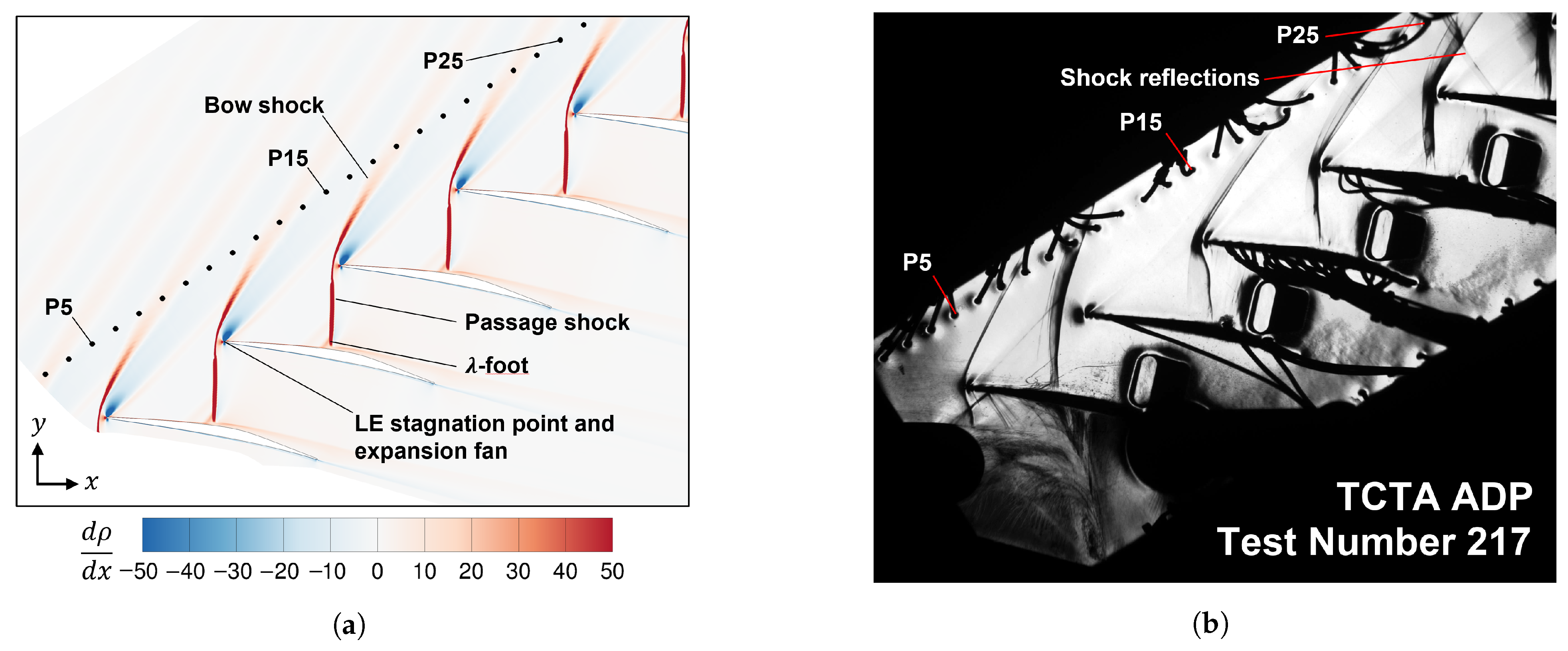
As a final step, the numerical Schlieren contour based on the density gradient along the
x-axis is compared in
Figure 6 with a snapshot of the Schlieren video taken at the TGK for TN 217. This TN corresponds to the same operating conditions as the ones presented for TN 125 in
Figure 4b. The computational domain has been extended and rotated to the same angle as the cascade in the wind tunnel. Additionally, the line of pressure taps has been added at the MP1 and labeled for reference. The topology of the flow is labeled in
Figure 6a and matches well with the one observed in
Figure 6b for the bow and passage shock directly adjacent to the middle passage. However, some of the main differences with the ideally periodic case can be observed in the other passages due to the difficulty in adjusting the first passage and the reflections that can be observed in the upper passages.
5.3. Detailed Comparison Approaching Cascade Stall
One final comparison is performed in
Figure 7 between the numerical results obtained with an inflow angle of 147.3° and the experimental results at the highest inflow angle measured of 147.2°. This time, the results are also compared with the alternative SSG/LRR CFD solver. The simulations with both solvers at and near these points are characterized by a periodic numerical instability of about 4% of the mass flow at the outlet. The results have then been averaged over two cycles, as explained in
Section 3.2. Comparing the RANS results with each other first, the M
distributions are shown to be very similar. The major difference lies in the wake, with the SSG/LRR solver showing a considerably higher peak loss and a slightly larger wake. The
was calculated to be 0.156 and 0.177 in the SST and SSG/LRR simulations, respectively.
Compared to TN 112, it is observed that the RANS solvers struggle to capture the development of the M
distribution over the region of the shock. The experiment also shows the effect of the shock to start more downstream than the simulations. In
Figure 7b, the wake is shown to have a lower peak loss than both solvers, although the wake size seems rather comparable. These differences can be partially explained by the lower AVDR for TN 112, but probably not to the extent of the deltas observed. A final comparison is performed in
Figure 8 with Schlieren snapshots of the numerical results and the experimental footage gathered for TN 222 with similar conditions as TN 112. The same flow topology of the ADP still holds, although notably, the
-foot is bigger, and the shock structure has shifted away from the leading edge. Some aperiodicity is also noticed for this operating point, but this time in the upper passages, which are inevitably throttled at this high inflow angle configuration.
6. Conclusions and Perspectives
In summary, the Transonic Cascade TEAMAero has been tested at the DLR’s transonic cascade wind tunnel over a variety of operating conditions across its entire working range. For this purpose, the cascade was manufactured and fully instrumented at the inlet, the blade surfaces, and the outlet. The measurements obtained agree well with the CFD-RANS results, with regard to the overall performance of the cascade. The measurements also confirm the successful achievement of the main objectives set in the original optimization of the new cascade design. These achievements include a large working range of at least 2°, with low losses at the inflow design angle (), and at a high aerodynamic loading (). However, some discrepancies with the CFD-RANS results become evident as the details of the flow are compared over the different regions of interest. This includes discrepancies in the development of the flow over the laminar separation bubble formed under the passage shock and in the topology of the wake losses at the outlet.
From the results presented, it can be said that the optimization methodology used to design the cascade has been validated, given that it focused on its overall performance over the working range. However, the results have also highlighted the shortcomings of the RANS methods employed, as some of the details resulting from the inherently unsteady flow around the shock–boundary layer interactions were not properly captured. This can be particularly problematic for designers, as these effects were shown to play a role in the development of the flow downstream of the cascade. This role was also shown to be increasingly important as the inflow angle approaches the upper end of the cascade’s working range. Further studies with different CFD-(U)RANS methods and approaches focused on these operating conditions could then bring tangible benefits to future design efforts. While high-fidelity CFD methods may be able to capture some of these missing details, they remain far too expensive for the purpose of a design effort.
Regarding the experimental campaign as a whole, it was shown that there is a palpable benefit available from bringing numerical and experimental methods together. The approach followed in designing and testing the TCTA has enabled the validation of both sets of results by drawing on their strengths and identifying their shortcomings. As interest grows in mitigating the unsteady effects observed, further and deeper collaborations will be required that take advantage of both research methods. Only in this way could researchers start clarifying the physical mechanisms driving these effects, potentially unlocking the performance of these designs. It is precisely this knowledge gap that the DLR aims to address in the future, within the context of the TEAMAero consortium, with further investigations into the TCTA using unsteady measurement techniques and high-fidelity CFD simulations.
Author Contributions
Conceptualization, E.J.M.L., A.H., and S.G.; data curation, E.J.M.L.; formal analysis, T.O.; funding acquisition, A.H.; investigation, E.J.M.L., A.H., T.O., and S.G.; methodology, E.J.M.L., A.H., T.O., and S.G.; project administration, A.H. and V.G.; resources, A.H. and S.G.; software, E.J.M.L.; supervision, A.H. and V.G.; validation, E.J.M.L. and A.H.; writing—original draft, E.J.M.L.; writing—review and editing, E.J.M.L., A.H., T.O., S.G., and V.G. All authors have read and agreed to the published version of the manuscript.
Funding
This project has received funding from the European Union’s Horizon 2020 research and innovation program under EC grant agreement no. 860909.
Institutional Review Board Statement
Not applicable.
Informed Consent Statement
Not applicable.
Data Availability Statement
Cascade geometry and exact data figures are available upon request to the correspondent author.
Acknowledgments
The authors would like to thank Jasmin Flamm, Maurice Simon Kruck, Jonas Ersfeld, and Martin McNiff, who have worked tirelessly in the facility to bring the TCTA cascade from paper to reality.
Conflicts of Interest
The authors declare no conflict of interest. The funders had no role in the design of the study; in the collection, analyses, or interpretation of data; in the writing of the manuscript; or in the decision to publish the results.
Abbreviations
The following abbreviations are used in this manuscript:
| Acronyms |
| ADP | aerodynamic design point |
| L2F | laser-2-focus |
| MP | measurement plane |
| TCTA | Transonic Cascade TEAMAero |
| TGK | Transonic Cascade Wind Tunnel |
| TN | test number |
| WR | working range |
| Latin letters |
| AVDR | axial velocity density ratio = |
| DH | de Haller number = |
| FT | flow turning = |
| M | Mach number |
| t | cascade pitch |
| Greek letters |
| flow or cascade angle |
| total pressure loss coefficient = |
| Subscripts |
| 1 | flow property at the inlet |
| 2 | total pressure loss coefficient = |
References
- Cumpsty, N.A. Compressor Aerodynamics, 2nd revised ed.; Number Bd. 10 in Compressor Aerodynamics; Krieger Publishing Company: Malabar, FL, USA, 2004. [Google Scholar]
- Hergt, A.; Klinner, J.; Wellner, J.; Willert, C.; Grund, S.; Steinert, W.; Beversdorff, M. The Present Challenge of Transonic Compressor Blade Design. J. Turbomach. 2019, 141, 091004. [Google Scholar] [CrossRef]
- Hirsch, C. Advanced Methods for Cascade Testing. AGARDOgraph 1993, AGARD-AG-3, 35–59. [Google Scholar]
- Fourmaux, A.; Gaillard, R.; Losfeld, G.; Meauzé, G. Test results on the ARL 19 supersonic blade cascade. J. Turbomach. 1988, 110, 450–455. [Google Scholar] [CrossRef]
- Fleeter, S.; Holtman, R.L.; McClure, R.B.; Sinnet, G.T. Experimental Investigation of a Supersonic Compressor Cascade; US Air Force Syst Command Aerospace Res Lab ARL 75-0208; Aerospace Research Laboratories: Fisherman’s Bend, VIC, Australia, 1975. [Google Scholar]
- Flaszynski, P.; Doerffer, P.; Szwaba, R.; Kaczynski, P.; Piotrowicz, M. Shock wave boundary layer interaction on suction side of compressor profile in single passage test section. J. Therm. Sci. 2015, 24, 510–515. [Google Scholar] [CrossRef]
- Hergt, A.; Klinner, J.; Willert, C.; Grund, S.; Steinert, W. Insights into the Unsteady Shock Boundary Layer Interaction. In Turbo Expo: Power for Land, Sea, and Air; American Society of Mechanical Engineers: New York, NY, USA, 2022. [Google Scholar] [CrossRef]
- Schreiber, H.A.; Starken, H. Evaluation of blade element performance of compressor rotor blade cascades in transonic and low supersonic flow range. In Proceedings of the 5th International Symposium on Air Breathing Engines, Bangalore, India, 16–22 February 1981; pp. 61–67. [Google Scholar]
- Munoz Lopez, E.J.; Hergt, A.; Beversdorff, M.; Grund, S.; Steinert, W.; Gümmer, V. The Current Gap Between Design Optimization and Experiments for Transonic Compressor Blades. In Proceedings of the 15th European Turbomachinery Conference, Budapest, Hungary, 24–28 April 2023; Paper n. ETC2023-223. Available online: https://www.euroturbo.eu/publications/conference-proceedings-repository/ (accessed on 11 June 2023).
- Munoz Lopez, E.J.; Hergt, A.; Grund, S. The New Chapter of Transonic Compressor Cascade Design at the DLR. In Turbo Expo: Power for Land, Sea, and Air; American Society of Mechanical Engineers: New York, NY, USA, 2022. [Google Scholar] [CrossRef]
- Munoz Lopez, E.J.; Hergt, A.; Grund, S.; Gümmer, V. The New Chapter of Transonic Compressor Cascade Design at the DLR. J. Turbomach. 2023, 145, 081001. [Google Scholar] [CrossRef]
- Voß, C.; Aulich, M.; Kaplan, B.; Nicke, E. Automated multiobjective optimisation in axial compressor blade design. In Turbo Expo: Power for Land, Sea, and Air; American Society of Mechanical Engineers: New York, NY, USA, 2006. [Google Scholar] [CrossRef]
- Ashcroft, G.; Heitkamp, K.; Kügeler, E. High-Order Accurate Implicit Runge-Kutta Schemes for the Simulation of Unsteady Flow Phenomena in Turbomachinery. In Proceedings of the Fifth European Conference on Computational Fluid Dynamics 2010, Lisbon, Portugal, 14–17 June 2010. [Google Scholar]
- Menter, F.R.; Kuntz, M.; Langtry, R. Ten Years of Industrial Experience with the SST Turbulence Model Turbulence heat and mass transfer. Turbul. Heat Mass Transf. 2003, 4, 625–632. [Google Scholar]
- Langtry, R.B.; Menter, F.R. Correlation-based transition modeling for unstructured parallelized computational fluid dynamics codes. AIAA J. 2009, 47, 2894–2906. [Google Scholar] [CrossRef]
- Klinner, J.; Hergt, A.; Grund, S.; Willert, C.E. High-Speed PIV of shock boundary layer interactions in the transonic buffet flow of a compressor cascade. Exp. Fluids 2021, 62, 58. [Google Scholar] [CrossRef]
- Eisfeld, B.; Brodersen, O. Advanced turbulence modelling and stress analysis for the DLR-F6 configuration. In Proceedings of the Collection of Technical Papers—AIAA Applied Aerodynamics Conference, Monterey, CA, USA, 17–19 August 2005; Volume 1. [Google Scholar] [CrossRef]
- Schlüß, D.; Frey, C.; Ashcroft, G. Consistent non-reflecting boundary conditions for both steady and unsteady flow simulations in turbomachinery applications. In Proceedings of the ECCOMAS Congress 2016—7th European Congress on Computational Methods in Applied Sciences and Engineering, Crete, Greece, 5–10 June 2016; Volume 4. [Google Scholar] [CrossRef]
- Starken, H.; Schimming, P.; Breugelmans, F.A. Investigation of the Axial Velocity Density Ratio in a High Turning Cascade. In Turbo Expo: Power for Land, Sea, and Air; American Society of Mechanical Engineers: New York, NY, USA, 1975. [Google Scholar]
- Celik, I.B.; Ghia, U.; Roache, P.J.; Freitas, C.J.; Coleman, H.; Raad, P.E. Procedure for estimation and reporting of uncertainty due to discretization in CFD applications. J. Fluids Eng. Trans. ASME 2008, 130, 078001. [Google Scholar] [CrossRef]
- Schodl, R. Laser Dual-Beam Method for Flow Measurements in Turbomachines. In Turbo Expo: Power for Land, Sea, and Air; American Society of Mechanical Engineers: New York, NY, USA, 1974; number 74-GT-157. [Google Scholar]
- Ferri, A. Investigations and Experiments in the Guidonia Wind Tunnel. In Proceedings of the Hauptversammlung der Lilienthal-Gesellschaft für Luftfahrtforschung, Berlin, Germany, 12–15 October 1939; pp. 1–33. [Google Scholar]
- Priebe, S.; Wilkin, D., II; Breeze-Stringfellow, A.; Mousavi, A.; Bhaskaran, R.; D’Aquila, L. Large Eddy Simulations of a Transonic Airfoil Cascade. In Turbo Expo: Power for Land, Sea, and Air; American Society of Mechanical Engineers: New York, NY, USA, 2022. [Google Scholar] [CrossRef]
| Disclaimer/Publisher’s Note: The statements, opinions and data contained in all publications are solely those of the individual author(s) and contributor(s) and not of MDPI and/or the editor(s). MDPI and/or the editor(s) disclaim responsibility for any injury to people or property resulting from any ideas, methods, instructions or products referred to in the content. |
© 2023 by the authors. Licensee MDPI, Basel, Switzerland. This article is an open access article distributed under the terms and conditions of the Creative Commons Attribution (CC BY-NC-ND) license (https://creativecommons.org/licenses/by-nc-nd/4.0/).


 ,
, 


