Numerical Modelling of the 3D Unsteady Flow of an Inlet Particle Separator for Turboshaft Engines ^†

Abstract

Helicopter and turboprop engines are susceptible to the ingestion of debris and other foreign objects, especially during take-off, landing, and hover. To avoid deleterious effects, filters such as Inlet Particle Separators (IPS) can be installed. However, the performance and limitations of these systems have to be investigated before the actual equipment can be installed in the aircraft powerplant. In this paper, we propose different numerical methods with increasing resolution in order to provide an aerodynamic characterization of the IPS, i.e., from a simple semi-empirical model to 3D large eddy simulation. We validate these numerical tools that could aid IPS design using experimental data in terms of global parameters such as separation efficiency and pressure losses. For each of those tools, we underline weaknesses and potential benefits in industry practices. Unsteady flow analysis reveals that detached eddy simulation is the trade-off choice that allows designers to most effectively plan experimental campaigns and mitigate risks.

1. Introduction

The ingestion of dust, sand, and other debris is one of the most threatening issues for helicopter engines when operating in extreme conditions. Particles jeopardize the integrity of the internal components, potentially inducing blade erosion and combustor wall glazing [1,2]. Inlet Particle Separators (IPS) are one method to avoid particle contamination in helicopter and turboprop engines, and they have become popular thanks to their compactness, low pressure loss, and weight savings [3] when compared to other filtering systems such as vortex tube separators and inlet barrier filters [1,3]. The working principle of an IPS is quite simple; the unfiltered airflow, composed of a gaseous phase and a particulate phase, is directed through a bifurcating channel. The rapid change of curvature in the geometry forces the particle trajectories to change and concentrate only into a small part of the gas flow, while the remaining debris is separated by impingement onto the lateral surfaces and redirected towards a bypass channel. As a result, the air flowing into the main channel is cleaner, and the process can be enhanced either by increasing the geometry curvature or by introducing additional obstacles to the flow path, such as flaps. The described features are visualized in Figure 1 (left), which provides a schematic representation of the geometry inside an IPS built at the von Karman Institute for Fluid Dynamics (VKI). This model is designed for the latest generation of turboprop engines, in which the presence of additional barriers (the two flaps) fosters the separation process [4].

Despite the benefits of these filters, IPS designers need to tackle several issues, such as additional weight and drag, increased engine power requirements, the constant need for inspection, and supplementary costs for logistics and installation. Moreover, the IPS geometry has to be carefully defined to avoid excessive pressure drop in the flow path from the inlet to the outlet channel, which is turbulent, highly 3D, and unsteady.

In response to the industrial need for IPS characterization and validation, researchers have devoted a great deal of attention to assessing separation efficiency through sand injection tests [5,6] and to the aerodynamic characterization of the IPS using CFD tools [7,8,9]. Barone et al. [3,5,6] performed experimental characterization of a 2D IPS by injecting sand of various sizes. The procedure consisted of weighing the filtered sand and comparing it with the mass of the total number of particles entering the intake. However, the aforementioned studies are limited to a bidimensional test section in a vertically-designed wind tunnel. Connolly et al. [8] recently published the first 3D simulation of IPS behaviour, including both particle tracking and detached eddy simulation (DES) approaches. The simplified geometry from the previous studies of Barone et al. [3,5,6] was extruded to account for three-dimensional flow investigations. The results clarify many flow features that were previously uncovered. Nonetheless, the study focused on a simplified bifurcating channel with neither flaps nor complex 3D surfaces.

To the best of the authors’ knowledge, most studies available in the literature devote scarce attention to the filters actually installed in helicopter and turboprop engines, which are more complex in terms of geometry and unsteadiness. Moreover, there is no systematic exploration of the analytical and CFD approaches that can be employed in the preliminary IPS design phase to support and complete experimental campaigns.

Therefore, this paper aims to provide a set of numerical models for the aerodynamic characterization of an industrial IPS (Figure 1, right); these models have increased level of representativity for the flow and computational effort. The semi-empirical and steady-state models allow designers to carry out a preliminary assessment of the flow features at the boundaries of the domain (bypass, outlet, and inlet channel), while the unsteady simulations deepen the flow separation and other important phenomena. The different approaches are validated with experiments in terms of global parameters (pressure losses and separation efficiency) to ensure their potential for use in parallel with experimental campaigns. The final goal is to define the trade-off method for the IPS design phase, i.e., a high-fidelity approach which helps to reduce the time of experimental campaigns while at the same time being characterized by reduced computational effort to meet the most stringent industrial timescales.

The remainder of this paper is structured as follows. Section 2 describes the experimental apparatus used for determining the separation efficiency and pressure losses of the IPS system. The numerical setup is presented in Section 3, first discussing the CFD models and then the semi-empirical 1D model. The results presented in Section 4 provide insights into the validation of the numerical models and the unsteady flow features inside the IPS. Finally, Section 5 concludes the paper with a discussion on the numerical modeling of the system, underlining weaknesses and potential benefits of each model in industrial practice.

2. Experimental Layout

The IPS designed for testing (shown in Figure 2, left) is installed in the C3 facility at the VKI, which is depicted in Figure 3; this filter is the scaled test section of an IPS manufactured by Safran Helicopter Engines in the framework of the EU-supported IPANEMA programme (Inlet PArticle Separator Numerical ExperiMental Assessment). The rig is a blow-down facility fed by compressed air at 40 bar in a 72 ${\mathrm{m}}^3$ reservoir. This allows typical test runs of 5–10 min depending on the mass flow required in the rig. The inlet vessel has the main function of stabilizing the flow coming from the pressure line system. The filtered air and the air flowing in the bypass are discharged into two downstream vessels, where sand collection is easier and more efficient. Each of the vessels is equipped with a frame mounting a particle filter. The reason for using vessels at the exit of both streams is to reduce the velocity, lowering the inlet pressure required to achieve the target mass flow and allowing the particles to settle on the filters as the flow speed is reduced. The locations of the measurement sections are indicated in Figure 2 (right); the inlet (IN), outlet/mainstream (OUT) and bypass (BY) planes correspond to the same locations in which the boundary conditions for the CFD simulations are enforced.

The IPS is tested over a range of flow conditions as close as possible to the operating conditions of a helicopter or turboprop engine in harsh environments and/or off-design situations. In this facility, these conditions are realized mainly through variation of the inlet total pressure $p_{IN}^0$ and outlet Reynolds number $R{e}_{OUT}$, defined as follows:

$$R{e}_{OUT}=\frac{4{\dot{m}}_{OUT}}{\mu P_{OUT}},$$

(1)

where ${\dot{m}}_{OUT}$ is the mass flow rate, $\mu$ is the dynamic viscosity, and $P_{OUT}$ is the wetted perimeter, all of which are assessed in the cross-section at the outlet of the IPS (Figure 2, right). In order to compare different test cases, the reduced mass flow at the outlet can be defined as

$$G_{OUT}=\frac{{\dot{m}}_{OUT}\sqrt{T_{OUT}^0}}{p_{OUT}^0},$$

(2)

where $T_{OUT}^0$ and $p_{OUT}^0$ are the total temperature and pressure at the outlet, respectively.

The mass flow rates in the channels are measured with Venturi nozzles, while $R{e}_{OUT}$ is manually regulated using a butterfly valve located after the outlet mass flow meter. There is another control valve installed downstream from the bypass mass flow meter, which is operated automatically and sets the bypass ratio ($BPR$) at each test (visible in Figure 3). The $BPR$ is provided by the ratio of the mass flow rate measured in the bypass channel (${\dot{m}}_{BY}$) and the total mass flow rate injected at the inlet (${\dot{m}}_{IN}$):

$$BPR=\frac{{\dot{m}}_{BY}}{{\dot{m}}_{IN}}.$$

(3)

Moreover, the total quantities are measured in the upstream and downstream vessels during each test (locations depicted in Figure 2, right), allowing the total pressure losses ${\zeta }_{OUT/BY}$ to be calculated:

$${\zeta }_{OUT/BY}=\frac{p_{IN}^0-p_{OUT/BY}^0}{\frac{1}{2}{\rho }_{IN}{v}_{IN}^2},$$

(4)

where the subscripts for the total pressure $p^0$ indicate either the outlet (OUT) or bypass (BY) exit cross-section, while ${\rho }_{IN}$ and $v_{IN}$ respectively indicate the density and velocity measured at the inlet cross-section. To validate the numerical models, the relative total pressure difference $P{L}_{OUT/BY}$ is taken into account as follows:

$$P{L}_{OUT/BY}=\frac{p_{IN}^0-p_{OUT/BY}^0}{p_{IN}^0}.$$

(5)

Regarding the particles, within the scope of this paper only one size range is employed; more details will be presented in a future work. We selected soda lime glass microspheres of 20–30 $\mathrm{\mu }$$\mathrm{m}$ and density 2500 $\mathrm{k}$$\mathrm{g}$/${\mathrm{m}}^3$; due to their reduced size, they represent a critical test case. This fine sand is characterized by a Stokes number in the range of 2–5, computed as the ratio between the particle time and flow characteristic time. The experimental test matrix is summarized in

Table 1. Experimental test matrix.

Case	Total Pressure ${\mathit{p}}_{\mathit{IN}}^0$[ $\mathbf{Pa}$]	Reynolds Number ${\mathit{Re}}_{\mathit{OUT}}$	Reduced Mass Flow Rate ${\mathit{G}}_{\mathit{OUT}}\left[\frac{\mathbf{kg}}{\mathbf{s}}\frac{{\mathbf{K}}^{0.5}}{\mathbf{bar}}\right]$	$\mathit{BPR}$
1	127,700	580,000	14.2	28%
2	126,250	580,000	14.4	13%
3	139,804	710,000	15.9	6%
4	137,874	710,000	16.2	28%
5	138,793	710,000	16.0	13%
6	125,500	580,000	14.4	6%

. The separation efficiency $\eta$ is calculated as follows:

$$\eta =\frac{\mathrm{Weight}\mathrm{of}\mathrm{sand}\mathrm{recovered}\mathrm{from}\mathrm{the}\mathrm{bypass}\mathrm{channel}}{\mathrm{Total}\mathrm{weight}\mathrm{of}\mathrm{sand}\mathrm{injected}\mathrm{from}\mathrm{the}\mathrm{inlet}\mathrm{channel}}.$$

(6)

The uncertainty of the derived quantities (e.g., mass flow rate, pressure loss, separation efficiency, Mach and Reynolds number, etc.) are calculated using Taylor’s formula [10], while the absolute uncertainties of the measurement devices are defined through calibration. The uncertainty of the separation efficiency is strongly dependent on the uncollected mass of sand after each test, which is mainly caused by leakages and manufacturing imperfections.

3. Numerical Setup

For the success of an experimental campaign, it is necessary to forecast potential issues during the IPS testing. Analytical models can provide rapid assessment of the IPS flow conditions and allow for leaner design procedures, as the designer does not need to resort to CFD tools to verify the effect of small variations in the initial conditions or in the IPS geometry. In this paper, we propose a semi-empirical 1D model (Figure 1, right), which is combined with CFD data to enhance its accuracy. However, as the method does not resolve the physics inside the IPS, it should be used in conjunction with higher-resolution methods. For investigations on industrially relevant problems, Reynolds-averaged Navier–Stokes (RANS) simulations are most frequently used. However, their main limitation is that all quantities are averaged; therefore, the obtained information is limited to averaged fields, i.e., data on secondary statistics cannot be straightforwardly obtained via RANS simulations. On the other hand, unsteady RANS (URANS) can offer time-accurate solutions; however, these remain limited to the unsteady fluctuations in the mean quantities. Consequently, RANS statistical approaches might not be suitable for the description of the IPS system, which is characterized by 3D, turbulent, and unsteady separation regions. Time-resolved simulations such as DES and large eddy simulation (LES) are capable of resolving those areas; however, they are significantly more expensive in terms of computational cost, especially for high-resolution grids. Due to the high Reynolds numbers (Table 1) and large size of the IPS domain, direct numerical simulations are computationally prohibitive, and have not been performed. The commercial software programs Fluent 2021R2 and CFD-POST 2021R2 are used for simulations and postprocessing respectively, while the 1D model is implemented in Python 3.9.7.

3.1. CFD Models

As a first step, we generated several tetrahedral meshes, with the scope gradually increasing the resolution in the streamwise, transverse, and spanwise (x, y, and z) directions. The grids are refined in the areas with high curvature without refining the boundary layer region with prismatic layers, as this paper focuses on the core flow regions. The fact that the regions close to the walls are not resolved certainly implies some uncertainty in the identification of the exact separation points, and small reattachment bubbles and vortexes close to the walls are not well captured. Nevertheless, this modeling proves to be effective for representing the flow features inside the IPS (Figure 4 and Figure 5). Details on the generated meshes are available in

Table 2. Summary of the grids generated for the IPS numerical modeling, with statistics of mesh quality: x = streamwise; y = transverse; z = spanwise; AR = aspect ratio; OQ = orthogonal quality.

Cell Count	(x,y,z)	AR	OQ	${\mathit{y}}_{\mathit{avg}}^{+}$	${\mathit{y}}_{\mathit{max}}^{+}$	${\mathit{PL}}_{\mathit{OUT}}$	CPU Time
8 M	(500,80,200)	<20	>0.19	58.4	774	7.84%	$\varphi$
30 M	(875,125,350)	<23	>0.20	45.6	189	7.90%	$5\varphi$
50 M	(925,150,400)	<31	>0.12	41.6	159	8.05%	$13\varphi$
70 M	(1000,175,450)	<37	>0.15	37.0	143	8.36%	$20\varphi$
95 M	(1100,185,475)	<${10}^3$	>0.01	34.9	125	8.21%	$50\varphi$

; the values of $y^{+}$ refer to k-$\epsilon$ RANS calculations at $R{e}_{OUT}=580,000$, $p_{IN}^0=124,200\mathrm{Pa}$, $BPR=21\%$, and $G_{OUT}=14.4\frac{\mathrm{kg}}{\mathrm{s}}\frac{{\mathrm{K}}^{0.5}}{\mathrm{bar}}$. In the two extreme cases, i.e., the coarsest and finest grids of around 8 million (M) and 95 M cells, respectively, the mesh is overall refined by around two times in each direction. However, excessively refining the grid up to 95 M cells causes a reduction of the orthogonal quality, mainly related to the absence of inflation layers in the high curvature walls, which implies an increase of the aspect ratio in those areas. Nonetheless, the enhancement of the resolution of the boundary layer for the 95 M mesh would make the CFD solution too expensive from the computational viewpoint. By focusing on the $y^{+}$ distribution in the fluid domain, $y^{+}$ is shifted towards lower values for more refined meshes. Regarding the coarsest mesh (8 M), although the maximum $y^{+}$ value is quite high, only 4% of the cells have $y^{+}>300$, i.e., most of the domain is in the suggested limit for the k-$\epsilon$ model. Table 2 provides information on the relative total pressure losses ($P{L}_{OUT}$) and approximate computational time for the different grids. The latter is expressed as a function of the time needed for the RANS calculation with the 8 million cell mesh ($\varphi$), regarded as a common industrial practice; $\varphi$ is around 40 min with 64 CPU cores. The difference between $P{L}_{OUT}$ predicted by the coarsest mesh and the finest mesh is less than 5%.

Preliminary RANS simulations allow the initial LES resolution factor S [11] to be estimated as the ratio between the integral length scale and the grid size:

$$S=\frac{l_0}{\Delta }=\frac{k^{3/2}}{\epsilon \Delta },$$

(7)

where $l_0$ is the integral length scale, $\Delta =(\mathrm{cell}{\mathrm{volume})}^{1/3}$, k is the turbulent kinetic energy (TKE), and $\epsilon$ is the dissipation rate. Practically speaking, the resolution factor provides an indication of how many cells are surrounding an eddy of size $l_0$. This can provide only an initial estimate, as the length from the RANS computation is an approximation of the integral length scale specifically adapted for homogeneous isotropic turbulence. As a rule of thumb [12], S should be greater than 5 to resolve at least 80% of the TKE. By plotting the contours of S in the symmetry plane (Figure 4), it can be observed that the mesh resolution increases with the grid size, i.e., the area in yellow ($S>5$) in the separation region is wider.

The different grids can be analyzed by plotting the velocity streamlines and the normalized vorticity contours (Figure 5). In this study, the normalized vorticity $\overline{\omega }$ is defined as

$$\overline{\omega }=\frac{\omega H}{v_{IN}},$$

(8)

where $\omega$ is the vorticity magnitude, H is the inlet channel height, and $v_{IN}$ is the inlet velocity; $\overline{\omega }$ varies with $R{e}_{IN}$, and for these preliminary RANS simulations the ratio $v_{IN}/H$ is approximately 680. As depicted in Figure 5, all grids predict a separation bubble near the entrance of the bypass channel located in the collector and above the downstream flap. However, the vortexes have different sizes, and the unsteadiness of these phenomena suggests the impossibility of fully predicting the flow behaviour in the IPS with steady RANS simulations. Moreover, $\overline{\omega }$ has a very similar trend and value for all grids. Although Figure 5 and Table 2 demonstrate the grid convergence of the RANS computations, no accuracy conclusions can be drawn, as this analysis is limited to steady-state flow fields. Therefore, two meshes have been chosen to conduct the unsteady analysis and evaluate their differences. On the one hand, we selected the lowest resolution mesh (8 M), as it predicts the presence of vortical structures well and has an acceptable resolution factor S (Figure 4 and Figure 5). On the other hand, the fine mesh of 70 M cells is used for high-resolution LES and URANS, as the improvement in the resolution factor S from 70 M to 95 M is small and mainly related to low-turbulence regions. According to [13], the 70 M mesh is suitable for wall-modeled LES, as its number of grid points is proportional to $R{e}_L$ (Reynolds calculated using the longitudinal length of the IPS L). It is important to underline that neither this grid nor the finest mesh (95 M) is able to accurately resolve the boundary layer: a wall-resolved LES would require a number of grid points proportional to $R{e}_L^{13/7}$. The numerical and subgrid-scale parametrization requirements for a wall-resolved simulation are beyond the relevant computational capabilities, principally due to the high Reynolds number and complex geometry.

The technical details of the CFD cases are summarized in

Table 3. Numerical test matrix. PT = particle tracking. $p_{IN}^0$ in [Pa]; $G_{OUT}$ in $\left[\frac{\mathrm{kg}}{\mathrm{s}}\frac{{\mathrm{K}}^{0.5}}{\mathrm{bar}}\right]$.

Case	${\mathit{p}}_{\mathit{IN}}^0$	${\mathit{Re}}_{\mathit{OUT}}$	${\mathit{G}}_{\mathit{OUT}}$	$\mathit{BPR}$	Mesh	Model	CPU Time
1	127,700	580,000	14.2	28%	8 M	RANS, Steady PT	$\varphi$, $0.1\varphi$
2	126,250	580,000	14.4	13%
3	139,804	710,000	15.9	6%
4	137,874	710,000	16.2	28%	8 M	RANS, Steady PT	$\varphi$, $0.1\varphi$
5	138,793	710,000	16.0	13%		DES	$260\varphi$–$340\varphi$
6	125,500	580,000	14.4	6%		URANS, Unsteady PT	$80\varphi$, 190$\varphi$–260$\varphi$
7	124,200	580,000	14.4	21%	Table 2	RANS	Table 2
8	144,200	580,000	12.2	21%	8 M	RANS DES	$\varphi$ $280\varphi$
9	247,000	1,280,000	16.5	21%	8 M 70 M	RANS, URANS, DES RANS, URANS, LES	$\varphi$, $80\varphi$, $310\varphi$ $20\varphi$, $1450\varphi$, $4500\varphi$

, which provides information on the boundary conditions, mesh, turbulence models, and approximate computational effort. The latter increases nonlinearly with the Reynolds number, $BPR$, and $p_{IN}^0$; for this reason, a range of $\varphi$ values is indicated for cases 5 and 6 (unsteady particle tracking). The realizable k-$\epsilon$ model is chosen for the RANS and DES (hybrid RANS-LES) simulations, and wall modelling is used in order to remain consistent with the $y^{+}$ values of the meshes used. To characterize the particle-laden flow, Lagrangian particle tracking is enabled and a Rosin–Rammler particle distribution is defined to be as close as possible to the experimental campaign ($d_{min}=20 \mathrm{\mu }\mathrm{m}$ and $d_{max}=30 \mathrm{\mu }\mathrm{m}$). The Wall-Adapting Local Eddy Viscosity model is chosen for the LES, as it is suited to the complex wall-bounded flow in the IPS [14]. This approach represents the eddy viscosity with a local formulation based on the square of the velocity gradient tensor, and accounts for the effects of both the strain and the rotation rate of the smallest resolved turbulent fluctuations. As a result, no explicit filtering is needed and only local information is required to build the eddy viscosity. The convergence criteria for the residuals are set to ${10}^{-3}$. For the unsteady simulations, we monitored quantities such as static pressure and mass flow rate at the boundaries and volume average of the turbulent kinetic energy. The temporal resolution of the unsteady simulations ($\Delta t=1\times {10}^{-6} \mathrm{s}$) was chosen to maintain a CFL condition of order unity, even though implicit time schemes are used, and to capture in time most of the fluctuations of the turbulent eddies that are resolved in space by the different grids. Explicit time integration is not available for the pressure-based solver in Fluent. The monitors allow the minimum simulation time needed to reach convergence to be defined, i.e., $5\tau$; $\tau$ is the through-flow time, defined as the ideal time a fluid particle takes to go past all the IPS:

$$\tau =\frac{L}{v_{avg}}\approx 0.01\mathrm{s},$$

(9)

where $v_{avg}$ is the average velocity magnitude in the longitudinal direction and L is the longitudinal length of the IPS. The accumulation statistics for the unsteady characterization started after $5\tau$ and proceeded for at least $5\tau$. For clarity, the CPU time indicated for the unsteady simulations in Table 3 refers to a simulation time of $5\tau$. Regarding the unsteady particle tracking, around 15 million particles are injected during a time window of $(1/20)\tau$. The particles are dispersed in dilute conditions with small volume and mass fractions (<0.1%), and consequently one-way coupling between fluid and sand can be assumed. The first six cases in Table 3 correspond to the experimental cases in Table 1. Regarding case 7, all the meshes in Table 2 were tested. Case 8 was set with the highest inlet total pressure structurally allowed in the VKI facility. Case 9 was considered because it represents a limit condition in terms of Reynolds number; this case presents more critical flow behaviour with respect to the lower Reynolds number cases (as it will be discussed in Section 4.2),and for this reason it was chosen to validate both the low-resolution (8 M) and high-resolution (70 M) grids.

3.2. Semi-Empirical 1D Model

In the IPS focus of this paper, the flow is accelerated and forced through a geometrical restriction from the inlet to the outlet, while it is discharged past the bypass channel with an initial contraction followed by a diffuser. Therefore, we can simplify this IPS into a 2D nozzle system, shown in Figure 6, and solve the equations for compressible flows (1D Euler equations) to find a first approximation of the flow behaviour in the IPS. The flow has been modeled as steady-state and inviscid, and the total temperature is assumed to be constant during the filtering process. Moreover, the semi-empirical 1D model is non-isentropic, as the algorithm computes the losses inside the IPS channel with a modelling derived from the specific test section geometry. As inputs, the model receives the $BPR$, outlet mass flow rate ${\dot{m}}_{OUT}$, inlet total pressure $p_{IN}^0$, total temperature $T^0$ (assumed to be constant during the process), gas properties (specific heat ratio $\gamma$, specific heat at constant pressure $c_p$, air gas constant R), and geometrical features, i.e., the cross-section of the outlet, bypass, and inlet channels ($A_{OUT}$, $A_{IN}$, $A_{BY}$), the throat cross-section $A_{BY,T}$, and the ratio between the orifice diameter and pipe diameter $\beta$ (used in the calculation of the pressure losses). The user can set the desired convergence criteria for the iterations. The model returns the following variables: (1) the static-to-total pressure ratios $p_{OUT}/p_{OUT}^0$ and $p_{BY}/p_{BY}^0$; (2) the flow conditions at the boundary cross-sections (density, Mach number, and Reynolds number); and (3) the pressure losses at the bypass ${\zeta }_{BY}$ and outlet and ${\zeta }_{OUT}$, which are modeled as explained herein.

It can be observed that the total pressure loss can be written in general as the sum of two contributions, namely, the localized pressure losses and the distributed pressure loss. Distributed losses are verified to have a limited contribution to the overall losses (less than 1%), and can be neglected. Local pressure drops mainly occur in three locations, as shown in Figure 6: to a first approximation, the boundary layer effects and the separation phenomena can be neglected. The restriction in Area A (in green) causes most of the losses; however, the collector bend (Area C in light blue) and the small contraction before the diffuser in the bypass channel (Area B in purple) cause minor local pressure drops as well. The localized pressure drop in the bypass exit channel (Area B in purple) is always lower than the one affecting the flow past the outlet channel, and can be calculated as follows:

$$\Delta p_{BY}^0=0.3\left(\frac{1}{2}{\rho }_{BY,IN}{v}_{BY,IN}^2\right),$$

(10)

i.e., the pressure losses are 30% of the dynamic head, computed with the arithmetic average between inlet and outlet density and velocity. This approximation has proven to be valid only at low inlet total pressure, when the bypass pressure losses are not as high. This is the case of the VKI experimental campaign. If the pressure increases, the compressibility in that region is no longer negligible, and the losses due to boundary layer and separation become very high. The factor 0.3 in Equation (10) is the localized loss coefficient for elbows with a laminar Reynolds number [15], which works fine for a first approximation and is validated by CFD at low pressure.

As confirmed by CFD studies with respect to the flow passage towards the compressor (of primary interest from an industrial point of view), Area A accounts for 80% of the losses and Area C for almost 20%. The former can be simplified as a passage with an orifice. The prescription provided by the ISO [15] can be used to calculate the localized losses in this case:

$$\Delta p_{ORIF}^0=(1-\left(0.24\beta \right)-\left(0.52{\beta }^2\right)-\left(0.16{\beta }^3\right))ϵ\frac{1}{2}{\rho }_{IN}{v}_{IN}^2.$$

(11)

In Equation (11), $ϵ$ is the compressibility factor, which depends on the ratio of the pressures between the outlet and inlet channels.

On the other hand, the losses in Area C (Figure 6) can be visualized as two 90-degree bends without considering any flow swirl or vorticity induced by the collector geometrical shape. Therefore, we can write

$$\Delta p_{COLL}^0\approx 0.5\left(\frac{1}{2}{\rho }_{OUT}{v}_{OUT}^2\right).$$

(12)

The above formula proves to be valid at low pressure, and is almost independent from the Reynolds number. As the pressure increases, the algorithm fails to provide accurate predictions.

Finally, the pressure losses are provided by

$$\begin{array}{cc}\hfill & {\zeta }_{BY}\approx \frac{\Delta p_{BY}^0}{\frac{1}{2}{\rho }_{IN}{v}_{IN}^2},\hfill \end{array}$$

(13)

$$\begin{array}{cc}\hfill & {\zeta }_{OUT}\approx \frac{\Delta p_{ORIF}^0+\Delta p_{COLL}^0}{\frac{1}{2}{\rho }_{IN}{v}_{IN}^2}.\hfill \end{array}$$

(14)

4. Results

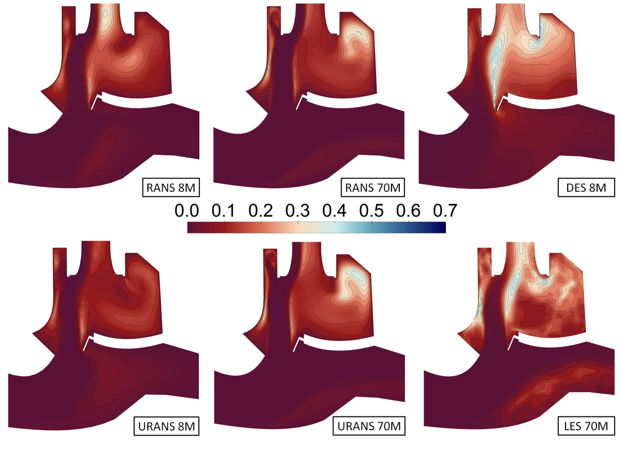
4.1. Validation of the Numerical Models

The aforementioned estimation of the resolution factor (Equation (7)) can only be used as an a priori calculation, and must be validated a posteriori by focusing on the ratio between the resolved TKE and total TKE from the unsteady simulations (DES and LES). Figure 7B,C depicts this ratio for the DES and LES simulations (case 9 in Table 3). Regarding the LES, in almost all the domains more than 95% of the turbulent kinetic energy is resolved, while the DES (performed with the 8 million mesh) has larger areas where the turbulent kinetic energy is less resolved, for instance, those above the two flaps and before the entrance of the bypass channel. Those regions are mostly assigned the RANS mode of solution, as indicated in yellow by the contour in Figure 7A. This contour is based on the calculation of a user-defined function (UDF):

$$UDF={\displaystyle \{}\begin{array}{cc}\hfill 0& \mathrm{if} l_{RKE}<l_{DES}\\ \hfill 1& \mathrm{otherwise}\end{array},$$

(15)

where the two length scales of the realizable k-$\epsilon$ and DES model are respectively provided by $l_{RKE}=k^{3/2}/\epsilon$ and $l_{DES}=C_{DES}$max($\Delta x$, $\Delta y$, $\Delta z$) = 0.61max($\Delta x$, $\Delta y$, $\Delta z$) (maximum local grid spacing).

The models are compared with experiments in terms of pressure losses and separation efficiency in

Table 4. Validation of the numerical models with experiments. Exp. = experiments; unc. = uncertainty. Cases 1,2,6: $R{e}_{OUT}=580,000$. Cases 3,4,5: $R{e}_{OUT}=710,000$.

Case		Separation Efficiency $\mathit{\eta }$ (%)				Pressure Loss ${\mathit{PL}}_{\mathit{OUT}}$ (%)
#	BPR	Exp.	Unc.	Steady Tracking	Unsteady Tracking	Exp.	Unc.	1D	RANS 8 M	URANS 8 M	DES 8 M
1	28%	78	±10	73	-	7.1	±1.3	7.33	7.11	-	-
2	13%	59	±8	63	-	6.8	±1.3	6.72	7.09	-	-
3	6%	49	±16	32	-	7.7	±1.2	8.28	8.53	-	-
4	28%	82	±12	72	89	8.5	±1.2	10.0	10.0	9.50	9.52
5	13%	64	±11	58	68	7.9	±1.2	8.77	9.74	9.41	7.92
6	6%	45	±10	21	46	6.7	±1.3	6.56	7.01	7.40	7.50

. Case 7 is not presented, as it has been already discussed (Table 2), while cases 8 and 9 are taken into account for the unsteady flow characterization.

Only the relative total pressure losses in the outlet channel ($P{L}_{OUT}$) are discussed, due to their greater influence on the overall engine performance with respect to those in the bypass channel. In fact, the pressure drop occurring in the mainstream channel directly affects the compressor operating point and its performance. It can be seen that $P{L}_{OUT}$ increases systematically as the bypass ratio increases, and the influence of the $BPR$ is more relevant at high Reynolds numbers. Although the experimental data may suggest that $P{L}_{OUT}$ increases with $R{e}_{OUT}$ for a given $BPR$, this trend cannot be confirmed by relying only on experiments; due to the facility’s architecture, the test conditions are realized by varying both $R{e}_{OUT}$ and $p_{IN}^0$ at the same time, and as such the effect of these two parameters is not decoupled. Nonetheless, the semi-empirical model confirms that for given $BPR$ and $p_{IN}^0$ the pressure losses increase with growing $R{e}_{OUT}$; this is related to the increase in $\Delta p_{ORIF}^0$ and $\Delta p_{COLL}^0$ (Equations (11) and (12)) as well. Moreover, for a given $BPR$ and $R{e}_{OUT}$, the model predicts a decrease in $P{L}_{OUT}$ as $p_{IN}^0$ increases. However, the theoretical model shows a larger difference with respect to experiments at higher Reynolds numbers ($R{e}_{OUT}=710,000$) and $BPR$ (>13%), as additional flow phenomena develop that cannot be captured by this 1D model, such as the separation bubble at the entrance of the bypass channel (as it will be discussed in Section 4.2).The pressure losses predicted by the steady-state RANS simulations are different from the experimental results at high Reynolds numbers and $BPR$, and they fall outside the uncertainty range in cases 4 and 5. On the other hand, the average pressure losses predicted by DES and URANS are closer to the experiments, overcoming the weakness of RANS modeling in characterizing the development of 3D flow instabilities at high Reynolds numbers and $BPR$. Moreover, the 1D semi empirical model and the steady-state CFD can be used only as preliminary design tools for $R{e}_{OUT}=1,280,000$ (case 9), as they prove inadequate in the estimation of $P{L}_{OUT}$ (underestimation of 15% compared to LES simulation). The average pressure losses from the URANS model are similar to those from high-resolution methods (DES for cases 4, 5, and 6 and LES for case 9); concerning case 9, it can be observed that the URANS calculations performed on two different grids (8 M and 70 M) show similar results (relative difference in $P{L}_{OUT}$ of less than 1%). For simplicity, the pressure losses in the bypass channel ($P{L}_{BY}$) are not shown; they are one order of magnitude less than $P{L}_{OUT}$, and show an increasing trend with increasing $BPR$. In the limit case $BPR$→0, both particles and airflow are directed towards the mainstream channel; hence, the pressure drop in the bypass channel becomes smaller and smaller ($P{L}_{BY}\to 0$).

Regarding the separation efficiency $\eta$ (Table 4), the outcomes of the experimental campaign show that the separation efficiency is harder to evaluate at low $BPR$ and high Reynolds numbers (higher uncertainty), as the amount of uncollected sand during tests increases; this negatively affects the validation process, especially at high Reynolds numbers. In these flow conditions, the RANS simulations with Lagrangian tracking loses accuracy and reliability; the solver does not fully converge, as particles remain trapped in the fluid domain. Therefore, RANS can only be used as an effective tool for the estimation of separation efficiency at high $BPR$. On the other hand, URANS coupled with unsteady particle tracking allows the separation efficiency to be predicted in better agreement with the experimental data, although it requires a longer computational time in order to let the injected particles escape from the bypass and outlet channel. It was observed that the particular shape of the collector further hinders the particles and makes the separation process more effective, as will be analyzed in a future publication.

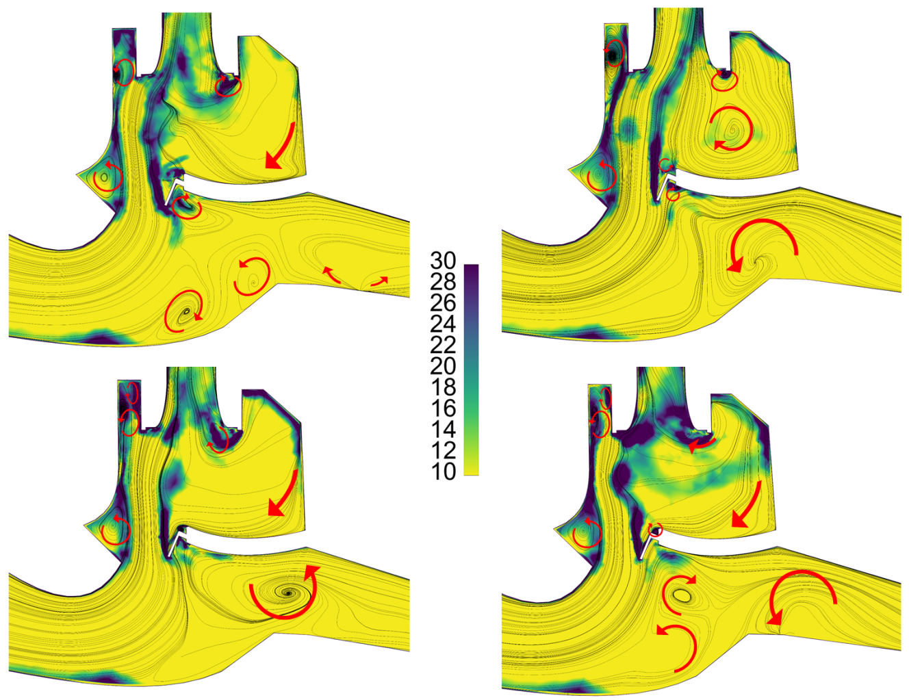
4.2. Unsteady Flow Characterization

Although the URANS model accords with the experimental data, the model validation cannot be limited to the global flow parameters. For this reason, the purpose of this section is to analyze several of the flow features inside the IPS at high Reynolds numbers ($R{e}_{OUT}=1,280,000$, case 9) in order to identify the weaknesses and strengths of each CFD model. The LES performed with the 70 M grid is taken as reference case; for brevity, we focus only on the dimensionless total TKE $\overline{k}$. The latter is computed as follows:

$$\overline{k}={\displaystyle \{}\begin{array}{cc}\frac{1}{v_{IN}^2}{k}_{avg}\hfill & \mathrm{for} \mathrm{RANS} \mathrm{and} \mathrm{URANS}\hfill \\ \frac{1}{v_{IN}^2}\left[k_{avg}+\frac{1}{2}(u_x^{\prime 2}+u_y^{\prime 2}+u_z^{\prime 2})\right]\hfill & \mathrm{for} \mathrm{DES}\hfill \\ \frac{1}{v_{IN}^2}\left[k_{sgs,avg}+\frac{1}{2}(u_x^{\prime 2}+u_y^{\prime 2}+u_z^{\prime 2})\right]\hfill & \mathrm{for} \mathrm{LES}\hfill \end{array},$$

(16)

where $u_x^{\prime }$, $u_y^{\prime }$, and $u_z^{\prime }$ are the respective velocity fluctuations in the x, y, and z directions, $k_{avg}$ is the average TKE, and $k_{sgs,avg}$ is the average subgrid-scale TKE from the WALE model. The definition of the total turbulent kinetic energy for LES and DES in Equation (16) assumes that the unsteadiness of the mean flow is negligible when compared to the turbulent fluctuations, as validated through URANS computations. Figure 8 depicts the total TKE $\overline{k}$ in the separation region (symmetry plane view). While the RANS models (both 8 M and 70 M) correctly identify the presence of turbulent flow structures above the two flaps, they underestimate the TKE of the separated flow, although the “improved” version of the k-$\epsilon$ model (realizable k-$\epsilon$ model) has been used here. Moreover, the location of the high-TKE region above the downstream flap changes with the mesh resolution, suggesting unsteady behaviour and indicating the inadequacy of steady-state methods. Furthermore, the URANS models show a number of differences compared to time-resolved methods such as DES and LES; these are mainly related to the very low magnitude of the captured velocity fluctuations (the resolved TKE is very small). On the other hand, the total $\overline{k}$ resolved by DES has the same magnitude as the high-resolution LES in the separation regions; the only areas where the model shows discrepancies with LES are those assigned to the RANS mode of solution (Figure 7A), i.e., close to the walls, in which unreliable gradients are predicted.

These considerations indicate that the flow in the IPS is highly turbulent and unsteady; therefore, the unsteady characterization cannot be limited to the mean flow quantities. Because of its considerably lower computational effort and relatively small difference with LES, DES has been taken into account for studying the instantaneous flow fields from the statistics accumulation; Figure 9 illustrates the development of the flow separation bubble at the entrance of the bypass channel when increasing $R{e}_{OUT}$. This instability is detrimental for the separation process, and represents an additional threat to the safe operation of the IPS. Designers should be aware of the unsteady development of the bubble as well as of the vortexes developing above the downstream flap (suggested by the streamlines and by the high vorticity regions in Figure 9). Focusing on planes perpendicular to the streamwise direction above the downstream flap, we observed that for both low and high Reynolds numbers (cases 8 and 9), the RANS and URANS simulations underestimated the local pressure and density drop, resulting in the evolution of these profiles (pressure recovery) being more optimistic than the one predicted by the mean of LES and DES.

As illustrated in the plot in Figure 10, the mean quantities are not enough to deeply describe the separation process, as the $BPR$ fluctuates over the acquisition window ($15\tau$–$20\tau$) with a frequency close to the through-flow frequency $1/\tau$ and the targeted $BPR$ (21%) cannot be kept constant throughout the whole separation process. The steady state simulations converge towards a mean $BPR$ of around 21%, while the unsteady simulations have slightly lower average values due to the captured mass flow rate fluctuations (which are minimal in case of URANS). Figure 11 indicates the evolution of several separation bubbles during (approximately) one oscillation cycle. All the 3D vortexes are projected onto the symmetry plane, and their directions are schematically depicted. During a cycle, there small corner vortexes develop and dissipate around the L-strut and downstream flap as well as in the curvature regions of the collector entrance (Figure 1). The vortex above the upstream flap suggests the generation of a horseshoe vortex in which the out-of-plane rotation is almost negligible. On the other hand, the two largest recirculation bubbles above the downstream flap and at the entrance of the bypass channel mostly deploy in the direction perpendicular to the symmetry plane. In particular, the bubble above the downstream flap is visible only at $t=16.25\tau$; therefore, this vortex does not having the same intensity along the out-of-plane direction. Last but not least, the vortical distribution at the entrance of the bypass channel shows that several bubbles develop perpendicularly to the depicted symmetry plane, and are characterized by different intensities. All of these features can influence the performance of the IPS in terms of separation efficiency and pressure losses.

5. Conclusions

Before actual installation in helicopter and turboprop engines, the IPS needs to be experimentally and numerically validated. This paper has shown how experimental campaigns can be supported and completed by employing different numerical models of increasing complexity. First, 1D semi-empirical models prove to be effective only for preliminary design calculations and planning of experiments, especially when the geometry of the IPS is not known in advance and the designer needs to perform further iterations to optimize the flow boundaries (inlet, outlet, and bypass). The 1D models fail to predict global pressure losses at high Reynolds numbers ($R{e}_{OUT}=1,280,000$) and $BPR$ (⪆20%), and for this reason have to be supported by CFD. RANS simulations are beneficial in terms of computational time, as they allow losses and separation efficiency to be estimated (though not in extreme conditions) with low effort. Thus, they have been widely employed to comply with stringent industrial timescales. Nonetheless, RANS offers only a limited overview of the separation phenomena occurring in the IPS, underestimating the pressure losses and neglecting the $BPR$ fluctuations. Moreover, RANS models such as k-$\epsilon$ show large discrepancies in their assessment of the turbulent kinetic energy in comparison with time-resolved simulations. A viable option for the estimation of separation efficiency and pressure losses is provided by URANS simulations, which require approximately 25% time less than DES for a given mesh, and more than three times less if unsteady particle tracking is not enabled. Although URANS has been successfully validated with experimental data, it is inaccurate for describing the unsteady behaviour of the IPS (underestimation of $\overline{k}$), as with the chosen turbulence model, time stepping, and spatial discretization the velocity fluctuations in the separation regions of the IPS are not well captured. In these core flow regions, DES and LES provide similar average results regardless of the mesh resolution; for this reason, DES can be implemented for a computationally affordable flow analysis. The possibility of visualizing and describing features such as separation bubbles and turbulent structures is highly valuable for the designers of industrial IPS systems as well as in view of test campaigns, as it is possible to move beyond the averaging process and obtain a large amount of information within a reasonable time frame. Therefore, DES is confirmed to be an efficient tool for characterizing IPS aerodynamics, as it allows the limitations of steady-state simulations to be overcome without the heavy computational effort and memory requirements of a high-resolution LES.

References

1. Filippone, A.; Bojdo, N. Turboshaft engine air particle separation. Prog. Aerosp. Sci. 2010, 46, 224–245. [Google Scholar] [CrossRef]
2. Hamed, A.; Tabakoff, W.C.; Wenglarz, R.V. Erosion and deposition in turbomachinery. J. Propuls. Power 2006, 22, 350–360. [Google Scholar] [CrossRef]
3. Barone, D.; Loth, E.; Snyder, P.H. Particle Dynamics of a 2-D Inertial Particle Separator. In Proceedings of the ASME Turbo Expo 2014, Düsseldorf, Germany, 16–20 June 2014. [Google Scholar]
4. Castaldi, M.; Mayo, I.; Demolis, J.; Eulitz, F. Numerical Modelling of the 3D, Unsteady Flow of an Inlet Particle Separator for Turboshaft Engines. In Proceedings of the 15th European Turbomachinery Conference, paper n. ETC2023-358. Budapest, Hungary, 24–28 April 2023; Available online: https://www.euroturbo.eu/publications/conference-proceedings-repository/ (accessed on 16 November 2023).
5. Barone, D.; Loth, E.; Snyder, P. A 2-d inertial particle separator research facility. In Proceedings of the 28th Aerodynamic Measurement Technology, Ground Testing, and Flight Testing Conference, New Orleans, LA, USA, 25–28 June 2012; p. 3290. [Google Scholar]
6. Barone, D.; Hawkins, J.; Loth, E.; Snyder, P.H. Inertial particle separator efficiency using spherical particles. In Proceedings of the 49th AIAA/ASME/SAE/ASEE Joint Propulsion Conference, San Jose, CA, USA, 14–17 July 2013; p. 3666. [Google Scholar]
7. Hamed, A.; Jun, Y.D.; Yeuan, J.J. Particle dynamics simulations in inlet separator with an experimentally based bounce model. J. Propuls. Power 1995, 11, 230–235. [Google Scholar] [CrossRef]
8. Connolly, B.J.; Loth, E.; Snyder, P.H.; Smith, C.F. Influence of scavenge leg geometry on inertial particle separator performance. J. Am. Helicopter Soc. 2019, 64, 1–12. [Google Scholar] [CrossRef]
9. Jiang, L.Y.; Benner, M.; Bird, J. Assessment of scavenge efficiency for a helicopter particle separation system. J. Am. Helicopter Soc. 2012, 57, 41–48. [Google Scholar] [CrossRef]
10. Taylor, J. Introduction to Error Analysis, the Study of Uncertainties in Physical Measurements, 1st ed.; 327 University Science Books: New York, NY, USA, 1997; p. 328. [Google Scholar]
11. Seifollahi Moghadam, Z.; Guibault, F.; Garon, A. On the evaluation of mesh resolution for large-eddy simulation of internal flows using OpenFOAM. Fluids 2021, 6, 24. [Google Scholar] [CrossRef]
12. Addad, Y.; Gaitonde, U.; Laurence, D.; Rolfo, S. Optimal unstructured meshing for large eddy simulations. Qual. Reliab. Large Eddy Simulations 2008, 12, 93–103. [Google Scholar] [CrossRef]
13. Choi, H.; Moin, P. Grid-point requirements for large eddy simulation: Chapman’s estimates revisited. Phys. Fluids 2012, 24, 011702. [Google Scholar] [CrossRef]
14. Nicoud, F.; Ducros, F. Subgrid-scale stress modelling based on the square of the velocity gradient tensor. Flow Turbul. Combust. 1999, 62, 183–200. [Google Scholar] [CrossRef]
15. ISO 5167-1:2003; Measurement of Fluid Flow by Means of Pressure Differential Devices Inserted in Circular Cross-Section Conduits Running Full—Part 1: General Principles and Requirements. ISO: Geneva, Switzerland, 2003. Available online: https://www.iso.org/standard/28064.html (accessed on 10 July 2023).
Figure 1. (Left) Schematic test section of the IPS built at VKI: 1, upstream flap; 2, downstream flap with an L-strut supporting the flap in the deployment phase; 3, collector. (Right) Numerical models presented in this paper.
Ijtpp 08 00052 g001
Figure 2. (Left) IPS geometry manufactured with 3D printing technologies. (Right) Detail of the test geometry, instrumentation location, and measurement sections.
Ijtpp 08 00052 g002
Figure 3. Global layout of the C3 facility (dimensions in mm).
Ijtpp 08 00052 g003
Figure 4. Resolution factor S (Equation (7)) for the meshes in Table 2. Preliminary RANS at R e O U T = 580 , 000 , p I N 0 = 124 , 200 Pa , B P R = 21% and G O U T = 14.4 kg s K 0.5 bar .
Ijtpp 08 00052 g004
Figure 5. Normalized vorticity magnitude contours (Equation (8)) and velocity streamlines for the grids in Table 2 (50 M mesh not shown for simplicity). Preliminary RANS at R e O U T = 580 , 000 , p I N 0 = 124 , 200 Pa , B P R = 21% and G O U T = 14.4 kg s K 0.5 bar .
Ijtpp 08 00052 g005
Figure 6. (Left) IPS schematized as a convergent nozzle in parallel with a convergent–divergent nozzle. (Right) The three main loss regions in the industrial IPS.
Ijtpp 08 00052 g006
Figure 7. (A): User-defined function UDF defining the regions in which the DES model switches to RANS (yellow). (B,C): Contours of the ratio between resolved turbulent kinetic energy and total turbulent kinetic energy (Case 9, Table 3).
Ijtpp 08 00052 g007
Figure 8. Contours of k ¯ (Equation (16)) for different models and mesh resolutions (Case 9, Table 3). The region of interest is the same as the one illustrated in Figure 9.
Ijtpp 08 00052 g008
Figure 9. Instantaneous ω ¯ contours ( t = 16.75 τ ) and velocity streamlines in the IPS regions between the two flaps from the mean of DES calculations (cases 8 and 9 Table 3) for two R e O U T . (Left) R e O U T = 710 , 000 ( v I N / H 680 ). (Right) R e O U T = 1 , 280 , 000 ( v I N / H 820 ).
Ijtpp 08 00052 g009
Figure 10. B P R in the IPS region depicted in Figure 9 at R e O U T = 1 , 280 , 000 .
Ijtpp 08 00052 g010
Figure 11. Instantaneous ω ¯ and velocity streamlines from the DES at R e O U T = 1 , 280 , 000 ( v I N / H 820 ) during one oscillation cycle. The red arrows schematically indicate the vortical directions. (Upper left) t = 16 τ . (Upper right) t = 16.25 τ . (Bottom left) t = 16.5 τ . (Bottom right) t = 16.75 τ .
Ijtpp 08 00052 g011