An Experimental Evaluation of Fault Diagnosis from Imbalanced and Incomplete Data for Smart Semiconductor Manufacturing


Department of Electrical and Computer Engineering, University of Central Florida, Orlando, FL 32816, USA
*
Author to whom correspondence should be addressed.
Big Data Cogn. Comput. 2018, 2(4), 30; https://doi.org/10.3390/bdcc2040030
Submission received: 18 July 2018
/
Revised: 10 September 2018
/
Accepted: 14 September 2018
/
Published: 21 September 2018
Abstract
:The SECOM dataset contains information about a semiconductor production line, entailing the products that failed the in-house test line and their attributes. This dataset, similar to most semiconductor manufacturing data, contains missing values, imbalanced classes, and noisy features. In this work, the challenges of this dataset are met and many different approaches for classification are evaluated to perform fault diagnosis. We present an experimental evaluation that examines 288 combinations of different approaches involving data pruning, data imputation, feature selection, and classification methods, to find the suitable approaches for this task. Furthermore, a novel data imputation approach, namely “In-painting KNN-Imputation” is introduced and is shown to outperform the common data imputation technique. The results show the capability of each classifier, feature selection method, data generation method, and data imputation technique, with a full analysis of their respective parameter optimizations.
1. Introduction
A semiconductor manufacturing process holds a colossal amount of data that are gathered from many sensors during the process. The gathered data contains valuable information regarding each produced entity, which can be used to gain knowledge about the yield of the production line, the failures that occurred and their results, and many other information that are crucial in operation of the semiconductor plant. Therefore, how this data is handled is of great importance.
Handling semiconductor data can be challenging. Firstly, a semiconductor manufacturing line holds many equipment and sensors, each being operational for long periods of time. Therefore, the amount of data that needs to be handled is large. Secondly, failures are rarely seen in this process. Being a highly expensive process, semiconductor industry has evolved to be inherently controlled on all front to lower the amount of failures that occur in the process. This fact gives rise to the challenge of imbalanced dataset, in which failure instances create a small portion of all observed instances. Thirdly, being an engineering process in the real world, missing data is common in the semiconductor manufacturing. Some parts of the data or specific feature might be missed due to malfunction or mismanagement, which creates the challenge for handling the missing data. Lastly, many of the signals that are recorded in the process do not have correlation to the classification at hand or are noisy. This fact creates a need for feature selection to find the most important values.
The SECOM dataset is a good example of semiconductor data. This dataset which holds data regarding instances that were a failure, is a highly imbalanced dataset, with many missing values, and noisy features. Therefore, this dataset creates an opportunity for realistic classification in the task of fault detection and diagnosis. Previous work has been done to classify this dataset to handle the imbalanced data and irrelevant features. In [1,2], the challenge of imbalanced data was evaluated and approaches for oversampling the minority distribution to create balance between the classes was introduced. In [3], the challenge of imbalanced data was evaluated from an under-sampling perspective as well, showing that oversampling performs better on this dataset. In [2,4,5,6] different approaches for feature selection were proposed to rise to the challenge of noisy features. The challenge of missing data remains unexplored in the SECOM dataset. To the authors’ knowledge, no literature thoroughly classifies the SECOM dataset after performing specialized data imputation.
In this work the SECOM dataset is classified using a plethora of combination of approaches. The three challenges of data imbalance, missing data, and noisy data are handled via synthetic data generation, data imputation, and feature selection, respectively. Moreover, different classifiers are evaluated, and their performance is analyzed based on the task at hand. To face the challenge of missing data, a novel data imputation technique called “In-painting KNN-Imputation” is introduced which is inspired by image in-painting. In the end, leveraging the feature importance delivered by the classification model, fault diagnosis is performed, that demonstrates which features and measured parameters during the manufacturing process have high effect on the failure of the device.
The rest of the paper is organized as follows. In Section 2 the background knowledge is provided. In this section, the semiconductor manufacturing, the manufacturing processes in this industry are conversed. The methodology of our work including the classification stages, the processes of data preparation, and procedures of constructing, evaluating, and interpreting the model for the data are discussed in Section 3. The designed and executed experiments and achieved results are catered in Section 4. The conclusion is given in Section 5.
2. Background
In this section, the general information and concepts regarding smart semiconductor manufacturing and this work are outlined.
2.1. Semiconductor Manufacturing Processes and the Data Volume
A sub-section of microelectronics is semiconductor manufacturing in which the “semiconductor wafers”, the substrates for semiconductor devices consisting of highly pure single crystal silicon, are processed in a fabrication facility using certain processing steps. The incorporating stages in processing these wafers can include: (1) Cleaning the wafer, in which the base of the semiconductor is cleaned. To accomplish this task, chemical substances are employed that can remove minor particles and residues made in the process of production or created by the exposure to air. (2) Deposition of film, in which thin film layers are formed on the wafer. Some of the common ways to perform this task are: (a) sputtering; (b) electro-deposition; and (c) chemical vapor deposition. (3) Cleaning after film deposition, in which the attached tiny particles to the wafer after the deposition of film are eliminated using physical-based methods such as spraying or brushing. (4) Resist coating, in which the surface of wafer is covered with photosensitive material for creation of resistivity on the wafer surface. The wafer is rotated by centrifugal force with the aim of creating a uniform layer of resistance on the wafer surface. (5) Exposure, in which the wafer is exposed to short wavelength deep ultraviolet radiations through a mask (containing the formed design patterns). (6) Development, in which the wafer is sprayed with the purpose of dissolving the exposed areas and consequently revealing the thin film on the wafer surface. (7) Etching, in which a pattern is created on the wafer by either: (a) excessive attacking on the wafer by ionized atoms for elimination of the film layer; (b) dissolving and removing the surface layer using chemicals (such as hydrofluoric acid or phosphoric acid). (8) Insertion of impurities, in which certain elements such as phosphor or boron ions are inserted into the wafer, creating the semiconducting properties. (9) Activation, in which the substrate is heated quickly via certain tools such as flash lamps. (10) Assembly, in which the output wafer is cleaned before it is separated into individual chips through dicing. (11) Packaging.
Each of the aforementioned stages have different types of sensors installed that can measure parameters of interest during the manufacturing process. These parameters that create the in-line data include measurements such as thicknesses of thin films after the processes of deposition, etching, or polishing, the crucial dimensions of wafer after applying the processes, film thickness and resistance, chamber pressure, flows of gases, temperatures of chuck, temperatures of the chambers, and so forth. Furthermore, other types of data are commonly gathered form different workstations, the manufacturing equipment, and the assembly stations. The collected data may belong to different parts ranging from raw silicon to final packaged product.
Through monitoring all the steps in semiconductor fabrication in the foundry, considering the number of stages and chambers, multiplied by the number of measurements in each stage, an immense amount of data is gathered. The data is not only large due to the complexity of processes, but also diverse due to the different sources that originate the collection of data.
While being large in size, the gathered data is highly valuable. Via using data analysis and machine learning methods, the gathered data is used in tasks of predictive maintenance, fault detection and classification, track manufacturing flow, real-time monitoring of the production process, and yield learning and improvement. Moreover, these methods can be used to extract useful information from a limited number of recorded occurrences to gain insight into the origins of each occurrence.
To fully take advantage of the data and implement the different aforementioned applications, the challenge of the collected data volume needs to be resolved. Analyzing a large corpus of data and making predictions based on it is a time-consuming task. This challenge is highly hindering in the semiconductor industry, since the time of delivery of products is of utmost importance and is a factor that affects the health and profitability of a semiconductor manufacturing plant. In the next section we present one of the applications of the gathered data which is the focus of this work, i.e., fault detection, and state its importance.
2.2. Fault Detection in Semiconductor Manufacturing
Traditionally, the production and the assembly lines are structured to build the devices and the products from raw material and elements. These material and elements are transformed and assembled with an increasing and gradual step to deliver end products and devices. This flow of products and devices from the beginning to the end of manufacturing line is not without flaws. Possible flaws to mention are breakdowns of machines, inconsistent processing times, and inaccessibility of operators and resources, and disturbances. The existing flaws challenge the way the production line operates and need to be faced to ensure profitability.
The key factors for companies and manufacturers within the semiconductor industry to be able to actively participate in the competition are cost, quality, and time of delivery of products. Monitoring and identifying the main and special characteristics of products in a timely manner and detecting the abnormalities at the right time during the manufacturing processes are essential tasks in this domain. Integrating modern technologies in this industry has enabled us to perform these tasks in real-time [7,8,9].
The large amount of data helps in improving the predictive maintenance problem (mainly when maintenance is needed for the equipment). Also, building a model for the task of fault detection and diagnosis is made possible using these data and the corresponding techniques. By making the task of fault detection and diagnosis timely, the downtimes of the machines are reduced, the companies burden less cost, and the quality of the products is guaranteed more.
There are other challenges with respect to the production environment and its dynamics. It is extremely important to have high yield across the entire line (more than 99% for each step of manufacturing process). On the other side, it is important to have as less waste (including product scrap, loss of production, environmental waste, general capital waste) as possible. Another challenging factor is the near-capacity operation of all the equipment and tools within the manufacturing facility. To resolve these challenges, a continuous data capturing, analyzing, and learning system should be established capable of maintaining the yields at high levels (based on the profit margins of the products). The system should also be able to detect and classify the faults and control the processes and predict the time for maintenance. Without a system such as this, the current demands and requirements in the semiconductor manufacturing will not be satisfied and as a result the devices and products will not have the sufficient quality for sale.
It is a requirement to perform diagnosis on the systems, tools, and equipment within a semiconductor industry to localize a fault and its root of cause and perform maintenance. Localization of a fault is done by looking into engineering models and determine if something goes wrong in the operation of every element in making a semiconductor device. Based on the determined fault model, the consequences of the occurring fault are determined.
2.3. SECOM Dataset
SECOM dataset first presented in [10], contains data gathered in a semiconductor manufacturing process. This data consists of 591 attributes and signals recorded throughout different trials, with each trial belonging to a production entity. Each trial would then be concluded by passing or failing an in-house testing line. Analyzing the data and finding correlations between failing the test and the attributes of the trial, enables engineers to firstly gain insight of why the failures occur, and secondly which attribute has the highest impact on the failure.
However, the SECOM dataset presents some challenges from a classification point of view:
- Overall 1567 trials were recorded, with only 104 of which resulted in failure. This creates a near 1:14 relation between the number of failures and successes recorded, resulting in a highly imbalanced dataset.
- Not all the signals that are recorded are useful for classification. Features exist in the SECOM dataset that present little to no data and do not change throughout the trials, moreover, some features exist that are very noisy or have no effect on the outcome of the test.
- Nearly 7 percent of the data in the SECOM dataset is missing. These data points were either never measured, or somehow lost and never made it to the final records.
3. Methodology
3.1. Classification System Architecture
Overall, three problems of data imbalance, unimportant features, and missing values exist in the SECOM dataset, which are prevalent in data gathered in a real-world process. In this work we use data imputation, synthetic data generation, and feature selection to overcome these problems and optimize the classification of SECOM dataset.
To begin with, the dataset needs to be cleaned. We delete features that have little to no effect on the outcome of classification, such as constant features or features with low variance, during the data pruning phase. After cleaning the data, the dataset is split into training and testing datasets. Next, the missing values are imputed using two approached of “Mean” and “In-painting KNN-Imputation”, the latter being an approach proposed by this work. Then synthetic data is generated to balance the classes of the dataset. Having done so, the task of feature selection is applied in different ways, to find the features that are most relevant and correlated with the outcome. Finally, the data is classified using four classifiers of Support Vector Machines (SVM), K-Nearest Neighbors (KNN), Random Forest (RF), and Logistic Regression (LR). A summary of these stages can be viewed in Figure 1.
Cross-Validation and the Proper Way to Do It
To present fair results and avoid over-fitting, ten-fold cross-validation is used in this classification system. To implement ten-fold cross-validation, the dataset is divided into ten sections. Having done so, one of the sections is chosen as the test set, while the remaining nine sections are considered as training sets. This process continues via choosing the next section as the test set, until all ten sections have been considered as the test set. Therefore, in the end, all the instances inside the data set have been tested and all the data has been viewed.
While examining several related works that perform classification on the SECOM data set via a pipeline of preprocessing stages, it can be seen that many choose to apply some or all the preprocessing on the data before splitting the data into training and test data sets. In [3,4,5], the task of feature selection was applied before cross-validation, and in [1,2,6,11] this task was applied before isolating one third of the data instances into the test set.
The repercussions of applying preprocessing tasks such as feature selection on the dataset with all the dataset as input can be huge on the classification results. In [12], a dataset is generated using 5000 columns of random values as features and 50 random values for the outputs consisting of two classes with the same size. Since the features are unrelated to the output, the true test error of any classifier is 50%, while via applying feature selection before splitting the data, they were able to achieve a 3% error rate. This huge gap between the real performance of the model and the achieved results comes from the fact that the feature selection stage has had access to all the data and has chosen features with the highest correlation to all the labels. This model would not be able to perform the same when new data is presented to it, rendering its results unreliable.
This fact holds true for other stages such as data imputation and synthetic data generation as well, which encourages one to bring those stages inside the cross-validation loop. In this work, the stages of data imputation, balancing the data, and feature selection, and classification are performed inside each fold of the ten-fold cross-validation, to avoid the leakage of data regarding the test data distribution into the training process. The data imputation stage is the only stage to have access to the test set, since it needs to fill the instances in that set as well; however, this stage will not use any information regarding the test data distribution, as described in Section 3.3.2.
To tune each stage, hyper-parameter tuning is done in the form of a loop inside each fold to find the optimum parameters. The details and results of each hyper-parameter tuning are presented in Section 4.
3.2. Data Pruning
In the 591 features present in the dataset, 7 features present no data since their value never changes. Moreover, after normalization of the dataset, 6 features have data distribution with a drastically low variance, such as features that are mostly constant in all cases but one. These features can be removed due to having very little information.
Furthermore, out of the near nine hundred thousand data points existing in the dataset, approximately sixty thousand data points are missing. The missing data points do not have a uniform distribution and some features or instances contain more of these missing data. The missing data can be viewed for each data instance (row-wise) in Figure 2a.
Since no instance shows a drastic amount of missing data, all the instances are kept, and no pruning occurs. The number of missing values for each feature (column-wise) can be inspected as well, which is shown in Figure 2b. As it is visible, a handful of features have more than 600 missing values. This fact renders those features useless, as the amount of information that remains available is not enough to base the classification upon or to extrapolate the missing values in these features.
Therefore, to prune the data, we delete feature columns that present no change, or those features that are beyond repair and have more than 600 missing values.
3.3. Data Imputation
After pruning the data, the amount of missing data points is decreased to 4.5 percent. While these features have missing values, they might hold important information that can affect the result of the failure test, so they cannot be simply deleted. Therefore, to deal with the problem of missing values, we need to apply imputation on the data. Imputation is the task of filling the missing values with real values that both have sensibility and maximize the expectation for the data point of interest.
In the literature, different approaches have been proposed for the task of data imputation. One approach is to completely delete any feature that contains missing data. In most cases, this approach which is known as “complete case analysis” will inevitably delete a part of the data that has high effect on the outcome of the classification, rendering the final model inefficient [13]. Moreover, the number of trials that are needed to achieve a higher accuracy is increased, since this data deletion will leave less data to infer upon for each trial. The most prevalent approach to data imputation is to substitute the missing values with the mean of the feature columns [14]. This type of imputation can distort the distribution of the feature vectors by changing their respective standard deviation [15]. Another approach that has been proposed for data imputation consists of models leveraging the local structure of the data to find the missing value. KNN-Imputation [15,16] is one of these approaches that uses KNN to predict the missing data point. In this work, inspired by image in-painting, we modify the approach of using KNN classifier for the task of data imputation.
3.3.1. Image In-Painting
When a picture is damaged, an artist is asked to repair the damage by in-painting the missing parts [17]. This task is performed on digital images as well, by looking at the values of each pixel. One can apply a median filter to the missing part and find out the approximate value of a pixel based on its neighbors. An implementation of image in-painting with the method introduced in [18] is shown in Figure 3.
Intuitively, a painter starts in-painting from the outer most regions of the missing section. This is because the painter is most confident as to what exists in those regions. In in-painting for digital images, one approach that can help increase the quality of the outcome is to choose the pixels that are on the outermost region of the missing section and predict their values first. The more neighbors that a pixel has, the more confident one can be about the value of that pixel.
Furthermore, a painter starts in-painting considering the familiarity of different parts of the missing regions. If one missing section is located on a low textured part of the image (i.e., the branches and body of the tree), and the other is located on a highly textured part of the image (i.e., the leaves), the painter perceives more familiarity in the low textured section and can predict the missing part with higher confidence.
3.3.2. Our Approach: In-Painting KNN-Imputation
In this work we try to use the concepts of “neighbors”, “confidence” and “familiarity” from image in-painting to predict the values of missing data and perform data imputation. This algorithm is shown in Algorithm 1.
While the neighbors of a pixel in an image are defined by proximity in location, the neighbors of a missing data point in a dataset can be defined by proximity using a distance metric. For example, by using Euclidian Distance, one can find data instances that are similar to the missing value, i.e., “neighbors”.
To define a metric of “confidence”, one can examine the dataset from the data instances and the features perspective. The more data points that are missing in a data instance, the less confident we are about the missing values in that instance. Moreover, the more missing values a feature column holds, the less confident we are about the value of the missing features. Therefore, we propose a metric of confidence for each missing value that consists of the summation of the number of the missing values in the column that holds the missing value of interest, and the number of missing values in the row of the missing value of interest.
To bring the concept of “familiarity” to our approach, the accumulative distance of the data instance to its “KNN” is calculated. If this data instance is an outlier, the instance is not familiar, and the calculated distance would be relatively large. On the other hand, if there are many instances existing in the dataset that are similar to the instance of interest, the calculated distance would be relatively small, and the instance would be a familiar instance.
| Algorithm 1 The Flow of Inpainting KNN Imputation. |
| Input Parameters: Input Data and Number of Neighbors (K-Param) Output Parameters: Filled Data Fetching Input: Data ← Read input data from file Calculating Number of Missing Values: for i in Columns do: NullSum[i] ← Sum(IsMissing(Data[:,i]) Iteration ← Sum(NullSum) Calculation of Confidence Value (Sum of Missing Values in Rows and Columns): Confidence ← 360 360 OneArray(DataDimension): for i in Rows do: RowSum ← Sum(IsMissing(Data[i,:])) ColumnSum ← Sum(IsMissing(Data[:,j])) for i in Rows do: for j in Columns do: if IsMissing(Data[0]) do: Confidence[i,j] ← RowSum[i] + ColumnSum[j] Familiarity = Sum(KNeighborsDistances): NNB ← NearestNeighbors(NeighborsNumber = KParam, DistanceOption = "Euclidean") FitForNNB(XArray) for i in Rows do: Distances = SumofDistances (KNeighborsForNNB (Data[i,:])) Familiarity[i] ← Distances Normalize Familiarity: FamiliarityNorm ← Normalized Familiarity Between [6, 360] Loop for Filling Missing Values: for Counter in Range(Iteration) do Order ← Confidence FamiliarityNorm Target ← argmin(Order): (x, y) ← Location of Target Extract Target Row for XTest: XTest ← Data[x,:] XTrain ← Remove row of "x" and column "y" from Data YTrain ← Extract column "y" from Data Delete Instances with Missing Values in the Target Column: Let Index be an empty array for Element in YTrain do: if IsMissing(Element) do: Removing row of element Filling Remained Part of XTest By Mean Values of Features: MeanTrain ← Mean(XTrain, Column) for FeatureCounter in Columns do: for InstanceCounter in Rows do: if IsMissing(XTrain [InstanceCounter, FeatureCounter]) do: XTrain [InstanceCounter, FeatureCounter] ← MeanTrain [FeatureCounter] for FeatureCounter in Range(Length(XTest)) do: if IsMissing(XTest [FeatureCounter]) do: XTest [FeatureCounter] ← MeanTrain [FeatureCounter] Predicting the Missing Value with KNN: Classifier ← KNeighborsRegressor(NeighborsNumber = KParam) FitForClassifier(XTrain,YTrain) Prediction ← ClassifierPrediction(XTest) for j in Column y do: Confidence[x,j] ← Confidence[x,j] − 1 for i in Row x do: Confidence[i,y] ← Confidence[i,y] − 1 Confidence[x,y] ← 360 360 Data[x,y] ← Prediction |
Having defined the metrics of “confidence” and “familiarity” and the concept of “neighbors”, an algorithm similar to image in-painting can be applied to impute the data. Using the multiplication of normalized confidence and familiarity, a metric is defined which helps choose the order in which data points should be filled. Similar to how a painter starts in-painting from the sections that they are more confident about, using this metric data points with higher confidence and familiarity can be identified and filled first.
The task of imputation is done using KNN regression. To begin with, the missing data point (X0, Y0) with the highest confidence and familiarity is found. The output of the regression would be the missing value that fills this data point, considering the values inside the feature column Y0. To train the model, parts of the dataset, excluding the label column and the data instance row (X0), are given as input. Since at this point the dataset contains missing values other than the missing value of interest (X0, Y0) and the regression model does not work with missing values, the rest of the missing values in the training data are filled with mean value of their respective feature columns. On the other hand, if there are any other missing values in the feature column of interest Y0, their respective instances are deleted from the training data, since they cannot offer any information regarding the missing value of interest (X0, Y0).
After the training is done, the data instance row X0 is fed to the model and the missing value of interest is predicted and placed into the original dataset. This process repeats until all the missing values are filled.
Since this KNN regression is done once on the data for each missing value, it is beneficial to use parallel computing to calculate the nearest neighbors for each iteration, reducing the overall time the algorithm consumes.
In this work, this algorithm is first applied to the training datasets inside each fold of the cross-validation. Having filled the training data, one instance from the test data is added on top of the filled data and the algorithm is applied again to fill the test instance. Then, the test instance is removed, and the same steps are taken for the remaining test instances. The reason for filling the training data and isolating it from test data, as well as isolating the test instances from each other, is to avoid letting any information regarding the distribution of the test data to be leaked into the imputation task.
3.4. Feature Selection
Having filled the dataset via data imputation, lack of missing values allows the task of feature selection to be carried on. This task is needed to delete unimportant and noisy features and to only keep the relevant data for the next stages.
Feature selection in this work is performed using four different approaches:
- Univariate feature selection: This type of feature selection performs univariate statistical tests on the input data and selects the ones with the highest scores. The scoring functions used in this work are Chi-squared (CHI2), ANOVA F-value between label and feature (FCLASSIF), mutual information (MFCLASSIF), false positive rate test (SELECTFPR), estimated false discovery rate (SELECTFDR), family-wise error rate (SELECTFWE).
- Selecting from a model: a group of estimators can output feature importance after they have been trained on the data. Using this feature importance, the highest-ranking features are selected from models such as RF, Logistic Regression with L1 (LR) and L2 (LR2) regularization, and Support Vector Machine with L1 (SVM) and L2 (SVM2) regularization.
- Recursive Feature Elimination (RFE): Similar to the previous approach, a model that outputs feature importance is fitted on the training data; however, the features with the lowest importance are removed. This process is repeated, and model is trained on the new data, until the features with the highest importance are remaining. The same models used for the previous approach are used for this approach (RFERF, RFELR, RFELR2, RFESVM, and RFESVM2).
- Dimensionality reduction: In this work Principle Component Analysis (PCA) is used to linearly reduce the dimensionality of the data, using Singular Value Decomposition of the data matrix to project each data vector to a space with lower dimensions.
Overall 18 different feature selection methods are evaluated.
3.5. Synthetic Data Generation
To tackle the problem of data imbalance, the relative number of the success instances need to become as same as or comparable to the relative number of success instances. This balance can be created either by oversampling the minority distribution—in our case the failures—or by under-sampling the majority distribution—i.e., the successes. Since oversampling has been shown to outperform under-sampling [3], we use oversampling in this work. The approach used in this work is Synthetic Minority Oversampling Technique (SMOTE) [19]. This technique is provided with the minority distribution, and it can generate a given number of new instances by sampling and interpolating among minority instances.
3.6. Classification
After the data is pruned, the features are selected, and the classes are balanced, the task of classification can be performed. Since the dataset is a structured dataset with binary classes, the four classifiers of LR, RF, SVM, and KNN are chosen and analyzed.
To validate our classification, we choose ten-fold cross-validation. Ten-fold cross-validation first partitions the data into ten sets, then the classifier is trained on nine sets and tested on one set. This process repeats until all folds have been tested. This approach results in avoiding over-fitting, since no special test set has been chosen, and all the dataset has been viewed and tested.
Cross-validation causes the training set to change every time a model is trained. However, to train each model, the training data needs to go through the stages of imputation, synthetic data generation, and feature selection. Therefore, these tasks need to be processed every instance the training data changes, inside each fold of ten-fold cross-validation.
4. Results
4.1. Experimental Setup
The data from the SECOM dataset goes through the stages of data pruning, data imputation, feature selection, and data boost and finally is classified using ten-fold cross-validation. All of stages are enabled using Python as software and four GeForce GTX 1080 graphic cards as hardware. The Scikit Learn tool [20] was leveraged in order to implement the feature selection stages. Overall, 288 different combinations of stages are examined, and the important results are reported hereafter. The main metric of evaluation in this work is area under the ROC curve (AUC), since this coefficient is a fair metric when classifying an imbalanced dataset. Another important metric of performance is recall in which the percentage of the faults that were caught is reflected. On the other hand, true negative ratio (TNR) indicates the percentage of successes that were rightly predicted and indicated how few false alarms were given by the classifier. Higher AUC, recall, and TNR indicated better classification.
4.2. Results
The existence of multiple stages in the classification pipeline encourages one to view the effects of each stage separately. In this section, the results are viewed objectively from each stage, comparing the performance of each combination within that stage. This comparison is done in two ways, firstly in the best delivered results for each approach by looking at the maximum AUC, secondly in the averaged delivered results between all approaches. The averaged result is computed by averaging the best results from the hyper-parameter tuning loop that contain the parameter of interest and not all the result from the loop. By doing this, we can keep one parameter constant and observe the best results it can deliver while other parameters change.
While comparing the best results will give insight into which combination of stages can deliver the best model, comparing the average results helps the fairness of generality in comparison by making each model compete in the same combination of stages.
4.2.1. Classification Results
To begin the task of classification, each model needs to be optimized considering the stages the data has passed through. The output of the KNN classifier is heavily affected by the number of neighbors (K). To find the optimum number of K, we classify the data using different values for K, and calculate the average of AUC for all classifications. This averaging allows us to find the optimum number of neighbors in the training set that need to be examined to make a fair prediction. Since the training set differs between the approaches using SMOTE or not, we average the two groups separately, as shown in Figure 4.
As it can be seen in Figure 4, the optimum value for K is equal to 1 in imbalanced data and is equal to 9 for balanced data. After applying SMOTE on the dataset and balancing the data, more data is available for the KNN model to infer upon. Therefore, in the balanced case, the model can rely on a higher number of neighbors to infer upon without the loss of performance.
This optimization can be done for the number of trees (N) in a RF model as well. Again, the value of interest is changed, and the average of AUC is recorded for the imbalanced and balanced data, as seen in Figure 5.
As it is visible in Figure 5, the optimum value for N is equal to 1 in imbalanced data and is equal to 3 for balanced data. As with KNN, more data is available in the balanced cases. Therefore, the RF model can build more trees on the data without the loss of performance.
To optimize the classifiers of SVM and LR, the inverse of regularization strength (C) can be changed. The lower this parameter is, the stronger regularization occurs. The result of changing C is reflected in Figure 6.
The optimum value for C for SVM, as seen in Figure 6, is 1 for balanced data and 10,000 for imbalanced data. A similar case is seen with LR, in which the optimum value for C is 10 for balanced data and 100 for imbalanced data. To understand the need for a bigger regularization parameter in the cases with imbalanced data, we need to examine the feature selection stage. In the cases of imbalanced data in this stage, the number of features that deliver better results in the classification stage are usually higher to preserve enough information regarding the minority class. Therefore, compared to the balanced cases, more features are kept and passed on to the next stages. This increase in the number of features that the classification stage receives necessitates a bigger regularization parameter.
To discover which classifier performed better, we average the results on all different approaches, as shown in Figure 7.
When comparing the performance of the classifiers using AUC, KNN fails to deliver good results in imbalanced cases, on the other hand, has the biggest increase in recall when the data is balanced. This is understandable due to the nature of this classifier that relies heavily on the data provided from a certain number of neighbors. SVM has delivered the highest average AUC both in the imbalanced and balanced cases, closely followed by LR.
Therefore, SVM is on average more capable of delivering classification results that are accurate in both success and failure classes. On the other hand, KNN has the highest recall, showing that this classifier is more capable of catching failures. Moreover, the highest TNR belongs to RF, implying that this classifier gives lower false alarms in general.
Choosing an optimized and trained classifier at this point depends highly on the preferences of the user of the model. In semiconductor manufacturing facilities, not capturing fault can be a costly mistake. Moreover, false alarms can be disruptive with prevalent fault detection systems; therefore, a balanced model is recommended, which can catch faults and still have few false alarms. Based on the results and comparing AUC, SVM and LR would be the preferred models.
The final results of each classifier with highest AUC reported in detail in Table 1.
As seen in Table 1, the best results in AUC were achieved by training an LR model. Therefore, LR is the superior model in this group of classifiers when considering the best performance. These results also show the superiority of In-painting KNN-Imputation to using mean value for imputation, since it has delivered the best results in all the examined models.
The best results achieved in this work are compared to the results from a similar work [21], which performs preprocessing after splitting the dataset into training and test set. This comparison is shown in Table 2.
As it is visible from Table 2, our model was able to have a higher recall while understandably a lower TNR. This higher increase is recall is arguably more valuable than the decrease in TNR when the task of fault detection is performed, resulting in more faults being discovered with an acceptable increase in false alarms.
4.2.2. Feature Selection Results
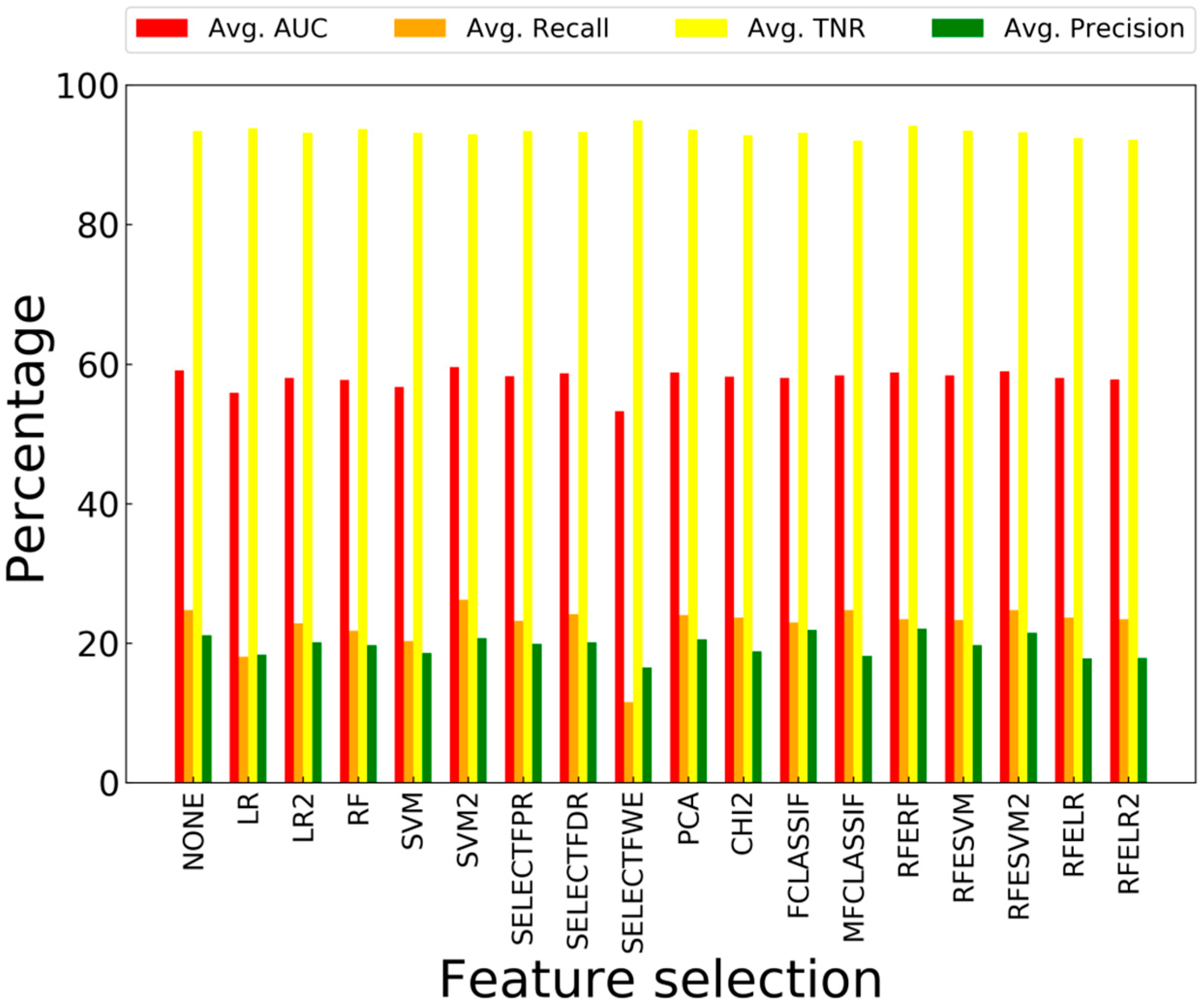
To evaluate the 18 different types of feature selection used in this work, similar to the previous section, we examine the average of the performance metrics, and the best performance of each approach in balanced and imbalanced cases. These results are shown in Figure 8, Figure 9, Figure 10 and Figure 11.
In both the balanced and imbalanced cases, SELECTFDR has given one of the best performances. The nature of SELECTFDR encourages the results to be in the favor of lower false discovery rate, therefore focusing on the identification of the positive class, i.e., faults.
As seen in Figure 8 and Figure 10, conducting no feature selection on the imbalanced data can yield one of the best results. When the data is imbalanced, more features have the potential to help represent the minority class and aid in discrimination of the small class from the large class, therefore feature selection might end-up hurting the end results. In the same figures it can be seen that alongside SELECTFDR, MFCLASSIF have shown good performance. MFCLASSIF relies on mutual info gathered from the classes and is adjusted to the size of the classes.
As seen in Figure 8 and Figure 9, on average SELECTFWE performance has the most improvement when the training data is balanced. This is because this feature selection approach uses family-wise error and the sizes of the classes have great effect on the outcome, making it unsuitable for the imbalanced cases.
As seen in Figure 9 and Figure 10, feature selection via SVM and LR can lead to high AUC and recall. Considering these results, the fact that these two classifiers had the best performance in the last section shows their suitability for discriminating the classes in the data distribution of the SECOM dataset.
4.2.3. Synthetic Data Generation Results
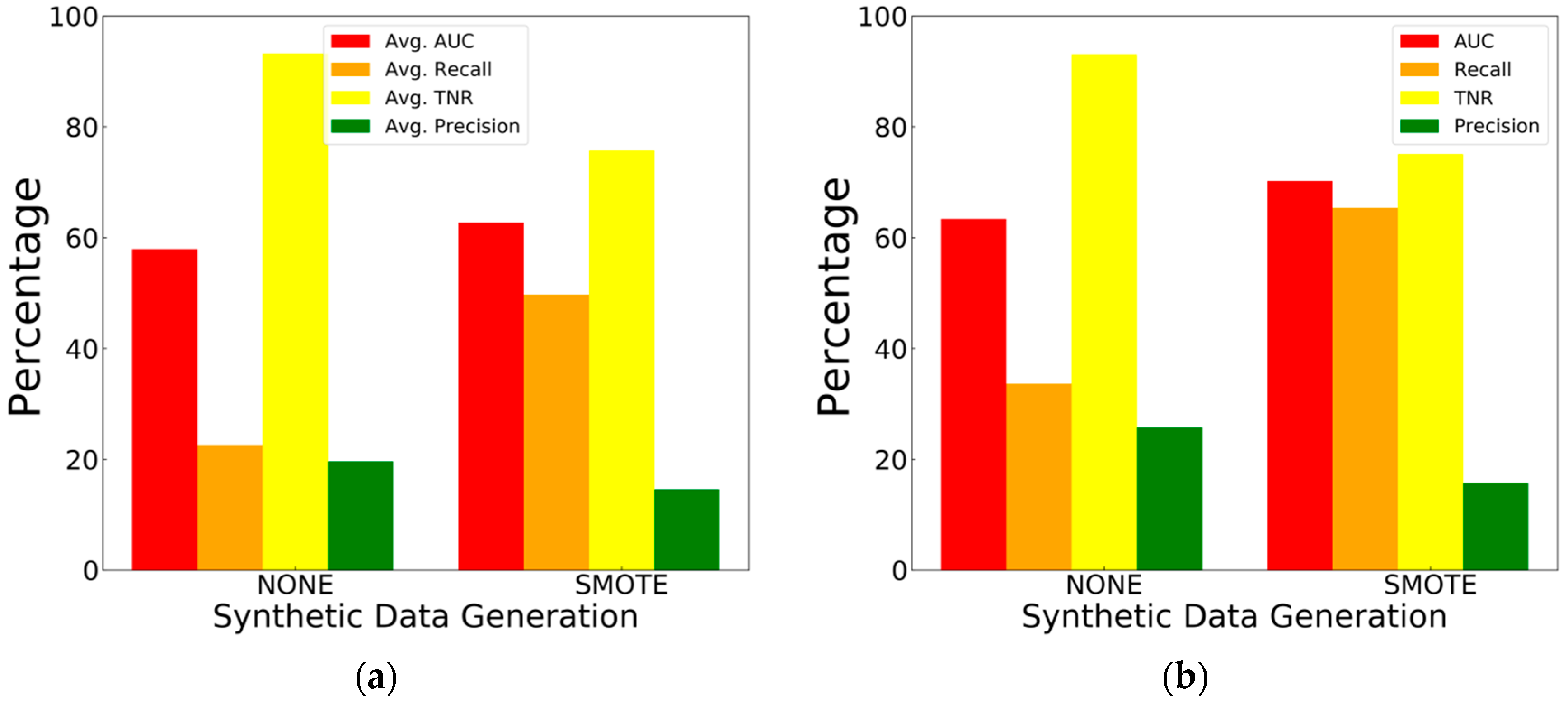
To evaluate the outcome of applying SMOTE on the dataset, the average and best performance of classification with imbalanced data and balanced data (using SMOTE) are compared in Figure 12.
Using SMOTE has resulted in a boost in performance via increasing AUC and recall. Since SMOTE creates a balanced training dataset, the models have a higher number of instances to train upon (compared to training on an imbalanced dataset), therefore, have a better understanding of the data distribution. A decrease in TNR is also visible which belongs to the trade-off between identifying more faults and having less false alarms. Therefore, the models trained on balanced data can classify more faults and deliver a better performance with acceptable change in the number of false alarms. These results show the importance of synthetic data generation.
4.2.4. Data Imputation Results
Training the KNN regression model relies heavily on the number of neighbors that are considered for regression (K). The number of neighbors is modified and the results, as shown in Figure 13, state that the best number of neighbors to consider for the regression and the familiarity metric is 3.
After finding the optimum number for K, the In-painting KNN-Imputation results are compared to imputation via replacing the missing values with the mean value of the feature vector. The results are shown in Figure 14.
While on average using mean value for imputation performs similar to In-painting KNN-Imputation, it is visible in Figure 14b that the best performance these approaches can give is highly different. In-painting KNN-Imputation has increased AUC and recall in the best approach, raising the limit our models could reach in performance.
To evaluate the metrics defined in our algorithm, the algorithm was implemented using three different order metrics (confidence, familiarity, and the multiplication product of both). In Figure 15, the performance of KNN-Imputation (regular) is compared to In-painting KNN-Imputation with these three different order metrics. The novel metrics of confidence and familiarity introduced in this work can each increase the AUC and recall of the original algorithm. By choosing the order metric as the multiplication of these two metrics, as introduced in Algorithm 1, the increase in AUC and recall are greater. This shows the effectiveness of In-painting KNN-Imputation since it results in models with better performance and higher probability in classifying a fault.
4.2.5. Feature Importance
Once the training is finished and the models are trained, it is possible to find out how important each feature is for each model and how much effect it has on the outcome of classification. The best model in this work results from In-painting KNN-Imputation, SELECTFDR feature selection, SMOTE data generation, and LR classification. By examining this model, the importance of each feature is observed.
SELECTFDR filters the p-values for an estimated false discovery rate from the p-values given to it. In this case, these p-values are delivered alongside the ANOVA F-values to the feature selection function. To compute the importance of each feature, the p-value for each feature is extracted inside each fold, and the average is calculated after the ten folds end. The average of the p-values is shown as importance in Figure 16.
Figure 16 reveals that the features that have the highest effect on the failures of the units are features 60, 104, 511, and 349. Via this approach, the root of the fault to failure is discovered, thus fault diagnosis is performed.
5. Conclusions
In this work, the SECOM dataset, containing data from a real-world semiconductor manufacturing plant, was examined and classified. During classification, 288 different approaches containing different stages for data imputation, data imbalance, feature selection, and classification were evaluated. Furthermore, a novel process for data imputation inspired by image in-painting was introduced. In the end, feature importance from the perspective of the best approach was analyzed, helping us gain insight to the result of failures and find the most crucial stages of the manufacturing line. By conducting this experimental evaluation, suitable tools and stages for classifying the SECOM dataset were identified, and the superiority of LR for classification, SMOTE for synthetic data generation, SELECTFDR for feature selection, and “In-painting KNN-Imputation” for data imputation were shown.
Author Contributions
M.S. formulated the idea, performed the simulations, and analyzed the results. S.T. reviewed the related literature, wrote the first draft, and drew the figures. J.-S.Y. formulated the problem, provided guidance in the writing of the manuscript, and reviewed the manuscript. All authors have proof-read the final manuscript.
Funding
This research received no external funding.
Conflicts of Interest
The authors declare no conflicts of interest.
References
- Kim, J.; Han, Y.; Lee, J. Data Imbalance Problem solving for SMOTE Based Oversampling: Study on Fault Detection Prediction Model in Semiconductor Manufacturing Process. Adv. Sci. Technol. Lett. 2016, 133, 79–84. [Google Scholar]
- Kim, J.K.; Cho, K.C.; Lee, J.S.; Han, Y.S. Feature Selection Techniques for Improving Rare Class Classification in Semiconductor Manufacturing Process; Springer: Cham, Switzerland, 2017; pp. 40–47. [Google Scholar]
- Moldovan, D.; Cioara, T.; Anghel, I.; Salomie, I. Machine learning for sensor-based manufacturing processes. In Proceedings of the 13th IEEE International Conference on Intelligent Computer Communication and Processing (ICCP), Cluj-Napoca, Romania, 7–9 September 2017; pp. 147–154. [Google Scholar]
- Kerdprasop, K.; Kerdprasop, N. A Data Mining Approach to Automate Fault Detection Model Development in the Semiconductor Manufacturing Process. Int. J. Mech. 2011, 5, 336–344. [Google Scholar]
- Wang, J.; Feng, J.; Han, Z. Discriminative Feature Selection Based on Imbalance SVDD for Fault Detection of Semiconductor Manufacturing Processes. J. Circuits Syst. Comput. 2016, 25, 1650143. [Google Scholar] [CrossRef]
- Kim, J.; Han, Y.; Lee, J. Euclidean Distance Based Feature Selection for Fault Detection Prediction Model in Semiconductor Manufacturing Process. Adv. Sci. Technol. Lett. 2016, 133, 85–89. [Google Scholar]
- Subramaniam, S.K.; Husin, S.H.; Singh, R.S.S. Production monitoring system for monitoring the industrial shop floor performance. Int. J. Syst. Appl. Eng. Dev. 2009, 3, 28–35. [Google Scholar]
- Caputo, G.; Gallo, M.; Guizzi, G. Optimization of Production Plan through Simulation Techniques. WSEAS Trans. Inf. Sci. Appl. 2009, 6, 352–362. [Google Scholar]
- Munirathinam, S.; Ramadoss, B. Predictive Models for Equipment Fault Detection in the Semiconductor Manufacturing Process. Int. J. Eng. Technol. 2016, 8, 273–285. [Google Scholar] [CrossRef]
- McCann, M.; Li, Y.; Maguire, L.; Johnston, A. Causality Challenge: Benchmarking relevant signal components for effective monitoring and process control. J. Mach. Learn. Res. 2010, 6, 277–288. [Google Scholar]
- Kim, J.K.; Han, Y.S.; Lee, J.S. Particle swarm optimization-deep belief network-based rare class prediction model for highly class imbalance problem. Concurr. Comput. Pract. Exp. 2017, 29, e4128. [Google Scholar] [CrossRef]
- Hastie, T.; Tibshirani, R.; Friedman, J.H. The Elements of Statistical Learning: Data Mining, Inference, and Prediction; Springer: New York, NY, USA, 2009. [Google Scholar]
- Gelman, A.; Hill, J. Missing-data imputation. In Data Analysis Using Regression and Multilevel/Hierarchical Models; Cambridge University Press: Cambridge, UK, 2006; pp. 529–544. [Google Scholar]
- Mockus, A. Missing Data in Software Engineering. In Guide to Advanced Empirical Software Engineering; Springer: London, UK, 2008; pp. 185–200. [Google Scholar]
- De Silva, H.; Perera, A.S. Missing data imputation using Evolutionary k- Nearest neighbor algorithm for gene expression data. In Proceedings of the 2016 Sixteenth International Conference on Advances in ICT for Emerging Regions (ICTer), Negombo, Sri Lanka, 1–3 September 2016; pp. 141–146. [Google Scholar]
- Troyanskaya, O.; Cantor, M.; Sherlock, G.; Brown, P.; Hastie, T.; Tibshirani, R.; Botstein, D.; Altman, R.B. Missing value estimation methods for DNA microarrays. Bioinformatics 2001, 17, 520–525. [Google Scholar] [CrossRef] [PubMed] [Green Version]
- Guillemot, C.; Le Meur, O. Image Inpainting: Overview and Recent Advances. IEEE Signal Process. Mag. 2014, 31, 127–144. [Google Scholar] [CrossRef]
- Biradar, R.L.; Kohir, V.V. A novel image inpainting technique based on median diffusion. Sadhana 2013, 38, 621–644. [Google Scholar] [CrossRef]
- Chawla, N.V.; Bowyer, K.W.; Hall, L.O.; Kegelmeyer, W.P. SMOTE: Synthetic Minority Over-sampling Technique. J. Artif. Intell. Res. 2002, 16, 321–357. [Google Scholar] [CrossRef]
- Pedregosa, F.; Varoquaux, G.; Gramfort, A.; Michel, V.; Thirion, B.; Grisel, O.; Blondel, M.; Prettenhofer, P.; Weiss, R.; Dubourg, V.; et al. Scikit-learn: Machine Learning in Python. J. Mach. Learn. Res. 2011, 12, 2825–2830. [Google Scholar]
- Chomboon, K.; Kerdprasop, K.; Kerdprasop, N.K. Rare class discovery techniques for highly imbalance data. In Proceedings of the International MultiConference of Engineers and Computer Scientists, Hong Kong, China, 13–15 March 2013. [Google Scholar]
Figure 1.
Overview of the diagnosis system architecture.

Figure 2.
Number of missing data points in: (a) Each instance; (b) Each feature.

Figure 3.
A sample of digital image in-painting: (a) Image with missing section; (b) Repaired Image after in-painting.
Figure 3.
A sample of digital image in-painting: (a) Image with missing section; (b) Repaired Image after in-painting.

Figure 4.
Average AUC when the value of K is changed in KNN classification on imbalanced data and on balanced data using SMOTE.
Figure 4.
Average AUC when the value of K is changed in KNN classification on imbalanced data and on balanced data using SMOTE.

Figure 5.
Average AUC when the value of N is changed in RF classification on imbalanced and balanced data.
Figure 5.
Average AUC when the value of N is changed in RF classification on imbalanced and balanced data.

Figure 6.
Average AUC when the value of C is changed in classification via: (a) SVM; (b) LR.

Figure 7.
Averaged results of each classifier on: (a) Imbalanced data; (b) Balanced data.

Figure 8.
Average performance of each feature selection approach on imbalanced data.

Figure 9.
Average performance of each feature selection approach on balanced data.

Figure 10.
Classification results with the highest AUC in each feature selection on imbalanced data.
Figure 10.
Classification results with the highest AUC in each feature selection on imbalanced data.

Figure 11.
Classification results with the highest AUC in each feature selection on balanced data.

Figure 12.
Classification results on balanced and imbalanced data: (a) Average of all approaches; (b) The best approaches (highest AUC).
Figure 12.
Classification results on balanced and imbalanced data: (a) Average of all approaches; (b) The best approaches (highest AUC).

Figure 13.
Classification results using different values for In-painting KNN-Imputation.

Figure 14.
Classification results on data filled with different imputation approaches: (a) Average of all approaches; (b) The best approaches (highest AUC).
Figure 14.
Classification results on data filled with different imputation approaches: (a) Average of all approaches; (b) The best approaches (highest AUC).

Figure 15.
Averaged classification results using different order metrics for KNN-Imputation.

Figure 16.
Importance of each feature.


Table 1.
Details of classification results with the highest AUC in each model.
| Classifier | Imputation | Feature Selection | True Positive | True Negative | False Positive | False Negative | TNR | Precision | Recall | AUC |
|---|---|---|---|---|---|---|---|---|---|---|
| LR | In-painting | SELECTFDR | 68 | 1098 | 365 | 36 | 75.05 | 15.70 | 65.38 | 70.22 |
| SVM | In-painting | SELECTFDR | 67 | 1104 | 359 | 37 | 75.46 | 15.72 | 64.42 | 69.94 |
| KNN | In-painting | SVM | 81 | 791 | 672 | 23 | 54.07 | 10.75 | 77.88 | 65.96 |
| RF | In-painting | SELECTFWE | 48 | 1152 | 311 | 56 | 78.74 | 13.37 | 46.15 | 62.45 |
Table 2.
Comparison of the results to a similar work [21].
© 2018 by the authors. Licensee MDPI, Basel, Switzerland. This article is an open access article distributed under the terms and conditions of the Creative Commons Attribution (CC BY) license (http://creativecommons.org/licenses/by/4.0/).
Share and Cite
MDPI and ACS Style
Salem, M.; Taheri, S.; Yuan, J.-S. An Experimental Evaluation of Fault Diagnosis from Imbalanced and Incomplete Data for Smart Semiconductor Manufacturing. Big Data Cogn. Comput. 2018, 2, 30. https://doi.org/10.3390/bdcc2040030
AMA Style
Salem M, Taheri S, Yuan J-S. An Experimental Evaluation of Fault Diagnosis from Imbalanced and Incomplete Data for Smart Semiconductor Manufacturing. Big Data and Cognitive Computing. 2018; 2(4):30. https://doi.org/10.3390/bdcc2040030
Chicago/Turabian StyleSalem, Milad, Shayan Taheri, and Jiann-Shiun Yuan. 2018. "An Experimental Evaluation of Fault Diagnosis from Imbalanced and Incomplete Data for Smart Semiconductor Manufacturing" Big Data and Cognitive Computing 2, no. 4: 30. https://doi.org/10.3390/bdcc2040030