
Optimization of Cryptocurrency Algorithmic Trading Strategies Using the Decomposition Approach
1
College of Computers and Artificial Intelligence, Helwan University, Cairo 11795, Egypt
2
College of Computing and Information Technology, Arab Academy for Science, Technology & Maritime Transport (AASTMT), Giza 12577, Egypt
*
Author to whom correspondence should be addressed.
Big Data Cogn. Comput. 2023, 7(4), 174; https://doi.org/10.3390/bdcc7040174
Submission received: 24 September 2023
/
Revised: 3 November 2023
/
Accepted: 9 November 2023
/
Published: 14 November 2023
(This article belongs to the Special Issue Applied Data Science for Social Good)
Abstract
:A cryptocurrency is a non-centralized form of money that facilitates financial transactions using cryptographic processes. It can be thought of as a virtual currency or a payment mechanism for sending and receiving money online. Cryptocurrencies have gained wide market acceptance and rapid development during the past few years. Due to the volatile nature of the crypto-market, cryptocurrency trading involves a high level of risk. In this paper, a new normalized decomposition-based, multi-objective particle swarm optimization (N-MOPSO/D) algorithm is presented for cryptocurrency algorithmic trading. The aim of this algorithm is to help traders find the best Litecoin trading strategies that improve their outcomes. The proposed algorithm is used to manage the trade-offs among three objectives: the return on investment, the Sortino ratio, and the number of trades. A hybrid weight assignment mechanism has also been proposed. It was compared against the trading rules with their standard parameters, MOPSO/D, using normalized weighted Tchebycheff scalarization, and MOEA/D. The proposed algorithm could outperform the counterpart algorithms for benchmark and real-world problems. Results showed that the proposed algorithm is very promising and stable under different market conditions. It could maintain the best returns and risk during both training and testing with a moderate number of trades.
1. Introduction
The crypto market environment has emerged as the most significant application of blockchain innovation in financial trading. Cryptocurrencies are advanced or virtual monetary forms supported by cryptographic frameworks. They enable secure online payment without the utilization of a third party or middleman. The term “crypto” refers to the different encryption calculations and cryptographic strategies that protect these payment operations. The crypto market is highly volatile due to the high fluctuations of asset values within a single day [1]. This volatility has a significant impact on the traders’ returns. That is why there is always a need for new, powerful algorithms that help traders improve their outcomes.
The cryptocurrency algorithmic trading models are classified into machine-learning-based models, portfolio optimization models, and trading strategy optimization models. Different researchers studied the deployment of a variety of machine-learning-based models in order to examine the predictability of cryptocurrencies using different time frames [2,3,4]. Gyamerah [5] proposed a hybrid model that uses both Support Vector Machine (SVM) and Technical Analysis (TA) tools to forecast the Bitcoin intraday price. In [6], Carbó investigated using machine learning techniques to identify the BTC pricing determinants. Deep learning models are also found in the literature in order to predict the fluctuations of cryptocurrency pricing; [7,8,9,10]. Portfolio optimization means the selection of the optimal portfolio or the optimal collection of assets from all those under consideration [11]. Portfolio optimization has been abundantly presented in the literature [11,12,13,14,15]. Trading strategy optimization means the optimization of the parameters of the trading rules used to examine historical trends in order to infer future behavior. With the help of one or more trading rules, the traders can determine the best entry and exit points, i.e., long and short positions. Karahan et al. [16] studied the incorporation of reinforcement learning as well as a collective decision optimization algorithm for Bitcoin (BTC) trading. The aim of their study is to maximize profits. Leung et al. [17] proposed an intelligent system for generating cryptocurrency trading signals that are developed using the sentiments exhibited in market tweets.
Despite its importance and widespread use, trading rule optimization is not frequently found in the literature. One of the main objectives of this research is to test the ability of optimized algorithmic trading strategies to hold on during different market conditions.
Cryptocurrency trading is a Multi-Objective Optimization (MOO) problem where there is more than one objective that needs to be optimized. Amongst these objectives are the return, the trading risks, the number of trades, the ratio between positive negative trades, the Maximum Draw-Down (MDD), which quantifies the maximum drop in an investment or asset’s value within a certain period, etc. [18].
The MOO problem can be described as shown in [19,20]:
where is the number of objectives, 𝛡 is the variable space or decision space, and F: is the objective space. The achievable objective set can be characterized as {}. Due to the conflicts among the objectives, the solution for such problems is not a single point, but rather a set of non-dominated points, i.e., the Pareto Set (PS) [21,22].
A solution is considered a non-dominated one when the advancement of one objective leads to the weakening of at least one of the other objectives. For any solution to be a Pareto Optimal (PO), it should not be dominated by another solution. It can be said that solution dominates another solution in the case that is not worse than for any of the objectives under study, and is better than B for at least one objective [21]. The Pareto Front (PF) is the set that is constructed by mapping the non-dominated points into the objective space, whereas the PS contains the PO points in the decision space.
The MOO algorithms can be categorized as algorithms based on Pareto-dominance and algorithms based on decomposition [20].
Multi-Objectives Evolutionary Algorithms using Decomposition (MOEA/D) is a promising algorithm used to resolve both multi- and many-objective optimization problems (i.e., MOO problems with ). Zhang and Li [21] first introduced MOEA/D to overcome the problems with dominance-based MOEAs, where they sometimes fail to handle many objective problems without a performance reduction. MOEA/D has demonstrated its simplicity and superiority in solving complex problems. It separates the complex MOO problem into a set of scalar Sub-Problems (SPs) with the help of a Scalarization Function (SF), also called an aggregation function. A set of well-generated weight vectors, as well as a finely selected SF, are the main factors that influence the performance of such an algorithm [21,22].
Due to the good performance shown by MOEA/D, different researchers have investigated some improvements to the original algorithm. The research studies for MOEA/D can be classified into four different categories: weight-generation strategies, the adaptation of one or more SFs, the implementation of different variants of the original algorithm to solve the challenges of more complex problems, and the application of MOEA/D algorithms to real-world problems.
Some new Pareto adaptively weighted generation aspects have been presented, such as paλ-MOEA/D [23], AWD-MOEA/D [24], MOEA/D-AWG [25], and MOEA/D-URAW [26].
New decomposition mechanisms were also found in the literature, either by using new SFs, as shown in [27,28,29], or by using a collection of different SFs [30,31].
The decomposition method has been expanded to a larger number of EAs, such as MOEA/DD-CMA [32] and MOEA/D-ACO [33]. The employment of a variety of novel operators to manage the diversity-convergence tradeoff has also been found in the literature, such as Differential-Evolution (DE) [34], a Two-Phase with Niching mechanism MOEA/D-TPN [35], and Hierarchical Decomposition (HD) [36].
MOEA/D was also applied to different application areas, such as network routing [37], portfolio optimization [38,39], image segmentation [40], and aerospace applications [41].
This study aims to evaluate the ability of the decomposition-based algorithms to enhance the performance of the cryptocurrency trading rules to help traders and investors improve their outcomes and compare them with the original or standard trading rules over a hardly predictable market condition, i.e., the COVID-19 pandemic.
In this paper, a decomposition-based Particle-Swarm-Optimization (MOPSO/D) algorithm, using a new linearly normalized Augmented-Weighed-Tchebycheff (AWTCH) scalarization method, has been proposed and applied to cryptocurrency trading strategy optimization. The AWTCH [42] is an updated version of the WTCH proposed by Zhang [21]. Normalization here is employed because the objective functions have extensively different ranges. The algorithm is used to optimize the controlling parameters of a set of four trading strategies named (Linear Weighted-Moving-Average, Bollinger-Bands, Stochastic Relative-Strength-Index, and Smoothed Rate-of-Change). In addition, a new hybrid weight generation strategy combining both systematic and random weight generation has also been proposed. The hybrid weight strategy is proposed to resolve the shortcomings of the systematic weight distribution proposed in [21] (as it fails to handle problems with complex PFs [20]) in a simple yet efficient methodology. The algorithm is trained and tested for the daily closing prices of Litecoin over two different periods. Litecoin was selected for two reasons. The first is that it can validate more transactions per unit time as compared to other cryptocurrencies. The second reason is that Litecoin has a low unit price, which makes it the best choice for novice traders.
The basic contributions of this research are:
- This research is the first to address using decomposition-based optimization strategies for cryptocurrency algorithmic trading.
- The proposed algorithm aims to find the best parameter set for each of the trading strategies in order to enhance the accuracy of the generated trading signals and avoid false signals.
- A new MOPSO/D has been proposed for the application at hand with two basic contributions, i.e., a newly proposed normalized aggregation mechanism and a new hybrid weight distribution mechanism.
- Furthermore, the algorithm is verified on some benchmark problems and compared against some state-of-the-art algorithms, such as the original MOEA/D and Strength Pareto Evolutionary Algorithm (SPEA2).
The following sections of this paper are organized as follows: Cryptocurrency algorithmic trading principles are shown in Section 2. The original MOEA/D algorithm is clarified in Section 3. The details of the proposed algorithm are presented in Section 4. The proposed hybrid weight generation strategy is presented in Section 5. In Section 6, the empirical results are shown, whereas the conclusions are viewed in Section 7.
2. Cryptocurrency Algorithmic Trading
Cryptocurrency investment involves a higher level of risk than other markets [43]. This risk arises from its volatile nature, where there is a wide range of fluctuations within limited time intervals [43]. The algorithmic trading of cryptocurrencies plays a crucial role in the world of digital currencies, providing numerous benefits and contributing to the market’s overall development and efficiency.
The algorithmic trading strategy used in this paper is accomplished with the help of four recommended technical indicators (TIs): Linear Weighted-Moving-Average (L-WMA), Bollinger-Bands (BB), Stochastic Relative-Strength-Index (St-RSI), and Smoothed Rate-of-Change (S-RoC). These indicators are mathematically based calculations that are used to generate trading signals (i.e., buy and sell signals) with the help of a set of controlling parameters [44].
These indicators are important for traders for many reasons:
- They are applicable for different types of markets, i.e., trending and sideways markets, such that the indicators are classified into overlay indicators and window oscillators suitable for trading and trending markets in sequence. The overlay indicators are lagging indicators (they are called lagging because the signals are generated based on price changes, such as Moving-Average (MA) indicators). The window oscillators are leading indicators (leading because the signals are generated prior to price changes, such as the RSI indicator) [44,46].
Each indicator has a set of standard parameters that were originally developed and recommended by its creator [49]. With different market conditions, there is no guarantee that these standard parameters could provide good profits or an acceptable level of risk [40]. Our aim here is to find the optimal indicators’ controlling parameters that simultaneously optimize the set of selected objective functions.
The L-WMA [41] is a Moving-Average (MA) indicator. MA indicators are used to find an updated price average, which helps to smooth and strip out the market’s sharp fluctuations. The L-WMA uses a previously decided weight value, which gradually decreases from the latest data point to the oldest one [50,51]. The greater the weighting factor, the more recent the pricing or data. The calculation for a L-WMA for an -days timespan is as follows:
Trading based on MAs is performed according to the crosses against the original price chart or against a longer-term MA. Crossing above the longer MA implies a long position (buy), while crossing below it implies a short position (sell) [51,52]. The standard n-values for double L-WMA are 20 and 50 days for short and long MAs, respectively.
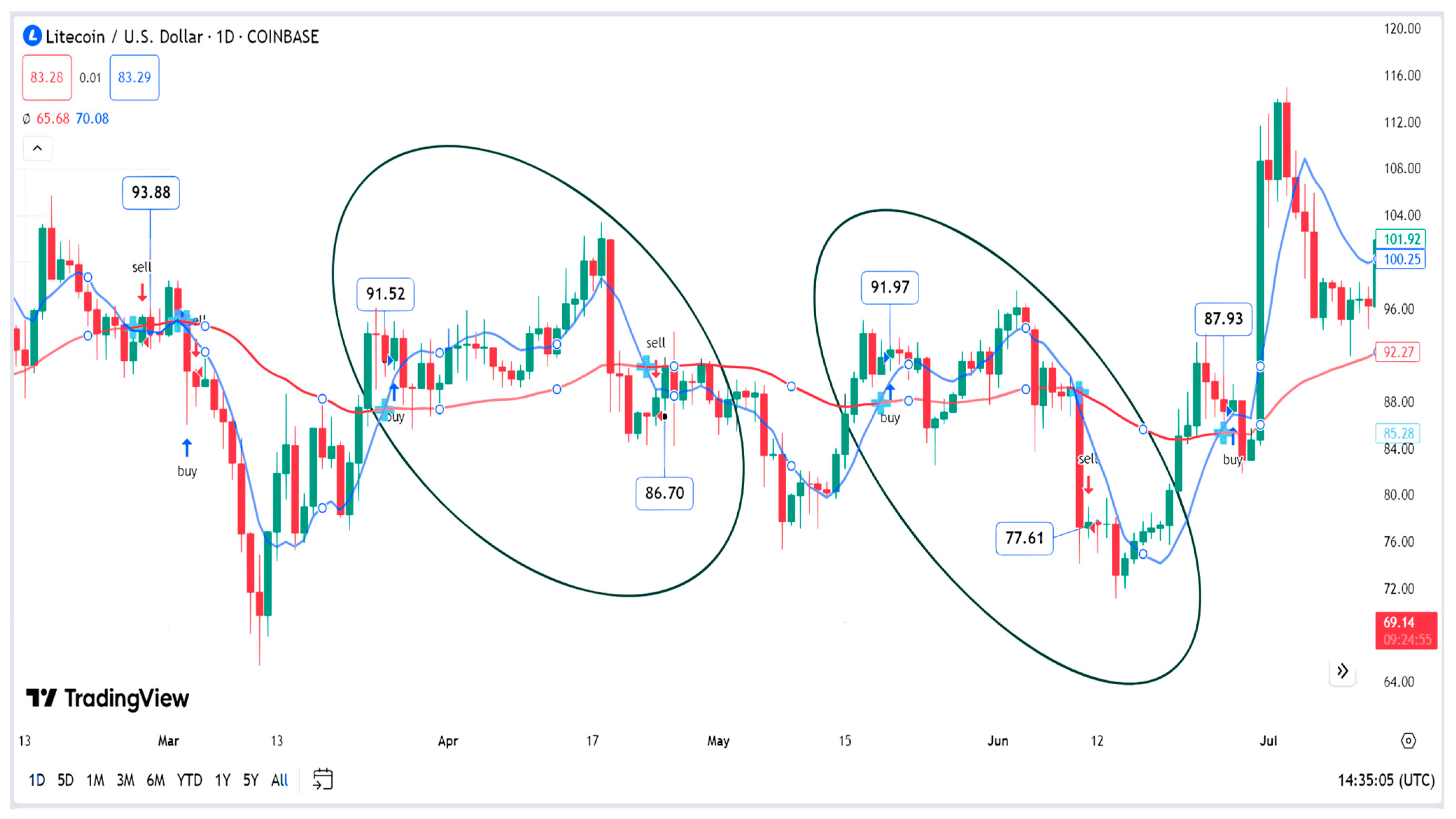
Figure 1 shows the effect of the chosen parameters for the L-WMA indicator on the final trading decisions. The two line charts represent the two L-WMAs, i.e., 20 and 50 days, while the bar chart is the daily price chart, where the color of the bar represents the rise or fall of the current price as compared to the previous one, i.e., red in case of a fall and green in case of a raise. As shown, there are many areas of false signals (shown in ovals). In these areas, the prices of buying are higher than those of selling, i.e., loss trade. This is due to the inability of the indicator’s parameters to reflect market changes. The smaller the number of days for the MA, the more sensitive the indicator is to market changes, but with more chances for false or wrong signals, i.e., high risk [44,53]. On the other hand, a larger number of days reduces the number of false signals at the expense of the sensitivity of the indicator, which in turn could generate many delayed signals and miss a large amount of profit [44]. This fact is common for all TIs. That is why the selection of the indicators’ parameters is a crucial decision in financial trading.
The BB [44] is a trading mechanism that employs two volatility bands: lower and upper bands, such that these bands are calculated as positive and negative Standard Deviations (STD) from a middle band. The middle band is typically calculated as the price Simple MA (SMA) (here, the Exponentially-MA (EXMA) is used instead in order to improve the accuracy). Trading using the BB is performed through the crossovers between the prices with the two volatility bands, i.e., the upper and lower bands [52,54].
The volatility of the bands is directly proportional to the STD, such that the bands expand with increasing volatility and contract otherwise [54]. The parameters that affect the BB indicator’s performance are the middle-band timespan , the STD lookback timespan , and the STD multiplier . The standard parameter values for the BB indicator are (20, 20, 2) for , and consequently. The three bands are calculated as shown below, where the is calculated the same as WMA with a higher weight on the latest data point, i.e., the current day, and equal weights on the rest of the days [44,53].
St-RSI [44] is a combined indicator that applies the Stochastic-Oscillator indicator to the RSI value, where RSI is another indicator that compares the change in the current price values to the prices of the recent past. The output is a value in the range between 0 and 100 that is used to determine the over-sold and over-bought layers. Upward and downward crossovers with these layers provide the buy and sell signals, consequently [52]. The value of St-RSI [44] is calculated as follows:
Such that is the RSI timespan, is the St-RSI timespan, and and are the average gains and losses during the past n-days. is the current RSI value whereas and are the maximum and the minimum values of the RSI during the past days. The standard St-RSI parameter values are (14, 14, 30, 70), such that the first two values are the values of both n and t, whereas the last two values are the values of the over-sold and over-bought levels in sequence.
The S-RoC [44] is also a combined indicator that applies the RoC to the EXMA value instead of the price data value. The output is a value in the range ±100. The power of this indicator is that it measures the trends’ strength by comparing the current EXMA value to the value of the EXMA calculated for the previous days. The S-RoC is calculated as shown:
The trading signals are generated through crossovers above and below a center line (typically a zero line) [52]. In this research, crossovers with over-bought and over-sold levels are used instead to generate trading signals. In this case, two additional parameters need to be optimized i.e., overbought and oversold levels. The standard parameter values for S-RoC are 14 days for the RoC calculation and 20 days for the EXMA.
These indicators have been selected in order to cover the two types of indicators, such that the first two (WMA and BBs) are classified as overlay indicators, whereas the last two (St-RSI and S-RoC) are classified as window oscillators [44].
During the optimization process, three objective functions have been considered: the Return on Investment (ROI), Sortino-Ratio (SOR), and the number of trades (TR). The ROI is the ratio between the net gain of the investment and the investment costs [55].
SOR is a statistical measurement used to evaluate the riskiness of an investment. It is one of the powerful tools used to evaluate the performance of the trading strategy, where high SOR values could reveal the stability of the selected strategy. It is calculated as the investment’s return relative to its downside volatility [56].
where r is the aggregated return value obtained by applying the trading strategy, is the risk-free rate, and is the downward standard deviation of returns.
The third objective function used is a calculation of the number of trades. The aim here is to minimize the number of trades, which in turn minimizes the trading costs.
The selected strategies are applied to the daily closing prices of Litecoin (LTC), which is one of the top three cryptocurrency trading volumes [18]. Two different time intervals were used. The first interval, starting from 3 January 2017 to 3 January 2019, was selected for training, while the second interval, starting from 3 January 2019 to 3 January 2021, was selected for testing, with 1460 data points divided equally between training and testing. These intervals were selected to test the robustness of the proposed methodology during the COVID-19 pandemic, as the crypto-market was highly influenced during that period [57].
3. Preliminaries of MOEA/D
In MOEA/D, the MOO problem is separated into a set of simultaneous single-objective Sub-Problems (SPs) with the help of an aggregation mechanism (i.e., a Scalarization Function (SF)). Several different SFs have been found in the literature. For example, Zhang [21] has evaluated three different SFs: Penalty-Boundary-Intersection (PBI), Weighted-Sum (WS), and Weighted-Tchebycheff (WTCH). Some other functions were also found in [28,30].
The Weighted Tchebycheff (WTCH), or weighted minimum-maximum, is one of the most suggested SFs as it is suitable for both convex and nonconvex problems [58]. As represented by Zhang [21], the PF of the MOO problem, shown in Equation (1), can be approximated by simplifying the problem into a set of SPs, such that the objective function of the SP can be shown as follows:
In [21], Zhang proposed a systematic weight distribution architecture, such that each weight vector , where H is a regulating integer parameter greater than 0. The number of SPs or weight vectors (such that denotes the mathematical combinations).
A neighborhood mechanism is employed such that each SP is optimized in accordance with its neighbors.
The neighborhood of the SP contains the set of SPs that have weight vectors distance away from , where is the neighborhood size. The basic steps of the original MOEA/D can be found in [21].
Due to the ability of the WTCH to solve various kinds of problems, different variants have been proposed to improve its performance [28,59]. The Augmented-Weighted-Tchebycheff (AWTCH) is one of the variants of the WTCH with a controlling parameter (ρ) that is provided in order to improve the quality of the generated non-dominated solutions and to avoid the weak optimal ones, such that ρ is a very small value in the range 0.001 to 0.1 [42]. The AWTCH is calculated as follows:
Some MOO problems have objectives that have extremely different ranges, which in turn affect the overall performance. So, different normalization processes have been found in the literature [60,61]. Linear normalization is a straightforward method that is simple and efficient. The result of this normalization process is that all the objectives will have the same range of values from 0 to 1. The linearly normalized form of the WTCH scalarization method (N-WTCH) is shown as follows:
Such that is the same as before, and is the minimum value of the objective space . As both and are not previously known, they are adaptively changed during each iteration [62].
4. The Proposed Algorithm
In this paper, a new decomposition-based Particle Swarm Optimization algorithm is proposed. The Normalized MOPSO/D (NMOPSO/D) is based on a linear normalization process to the AWTCH scalarization approach. The normalized form of the AWTCH (N-AWTCH) is calculated as:
The proposed algorithm (Algorithm 1) is used to optimize the parameters of a set of four algorithmic trading paradigms over three objective functions. The optimization process is performed using the MOPSO/D algorithm, where the algorithm first initializes the particles’ positions, velocities, and personal and global best positions. Each particle represents a separate SP, such that is the position of particle at time , while is the velocity of particle at time . For the application at hand, the particles’ positions are the indicators’ parameters. Each particle is assigned a weight vector that is used for fitness aggregation purposes. The Euclidean distance between each pair of particles, or SPs, is calculated in order to determine the particles that lie in the same neighborhood.
The evolution of the algorithm is obtained through a certain number of iterations. In order to find an optimum in the search space, the PSO formulation takes into account how the particles interact and move as a swarm. Over time, the particles cluster into an optimal location in the search space by using both exploration and exploitation. While the particles try to enhance or gain from the known promising locations through exploitation, the particles explore new areas of feasible space. Exploration and exploitation can be achieved and controlled during the velocity update through the inertia weight as well as the personal and global best constant accelerators ( and ). The inertia component is used for exploration principles as it is used to control the influence of the previous particle’s velocity, i.e., search direction.
The personal and global best accelerators are used for exploitation purposes, such that is the accelerator value that limits the step towards the particle’s personal best position , whereas is used to limit the step toward the global best position . The is the best position that the particle achieved through the past iterations (the one that provided the best-aggregated fitness).
| Algorithm 1: NMOPSO/D algorithm for cryptocurrency trading |
Inputs:
Steps: Repeat for each indicator: 1. Initialization:
For 2.1 Calculate the aggregation function: 2.2 According to the , update and . 2.3 Update the reference point . 2.4 Update the velocity as:
2.6 Apply mutation operator. 2.7 Repair. 2.8 Update the EA. 2.9 Update weight vectors W (Algorithm 2). 2.10 Update neighborhood . 3. If the stopping criteria is met, then stop. Else go back to step 2. 4. Return EA. |
The is the best obtainable position among the neighborhood of particle through the past iterations. To improve the exploration facility of the proposed algorithm and avoid premature convergence, a uniform mutation operator is applied to the particles’ positions and then the related data structures, i.e., , , and reference point are updated. In uniform mutation, the value to be mutated is exchanged with a new uniformly randomly generated value within the predetermined range of each variable [63]. As the mutation improves the diversity of the particles through the search process, it sometimes negatively affects their convergence. To improve the exploitation of the algorithm and ensure convergence, a repair strategy is proposed that re-evaluates the particle’s performance after mutation and ensures that it is not decayed; if so, the effect of the mutation is reversed, and the particle is returned to its previous position. An unbounded External Archive (EA) is used to hold the final non-dominated solutions found through the search process. Although using an unbounded archive increases computational complexity, it is very useful in keeping all the non-dominated solutions and not losing good solutions, which in turn improves diversity.
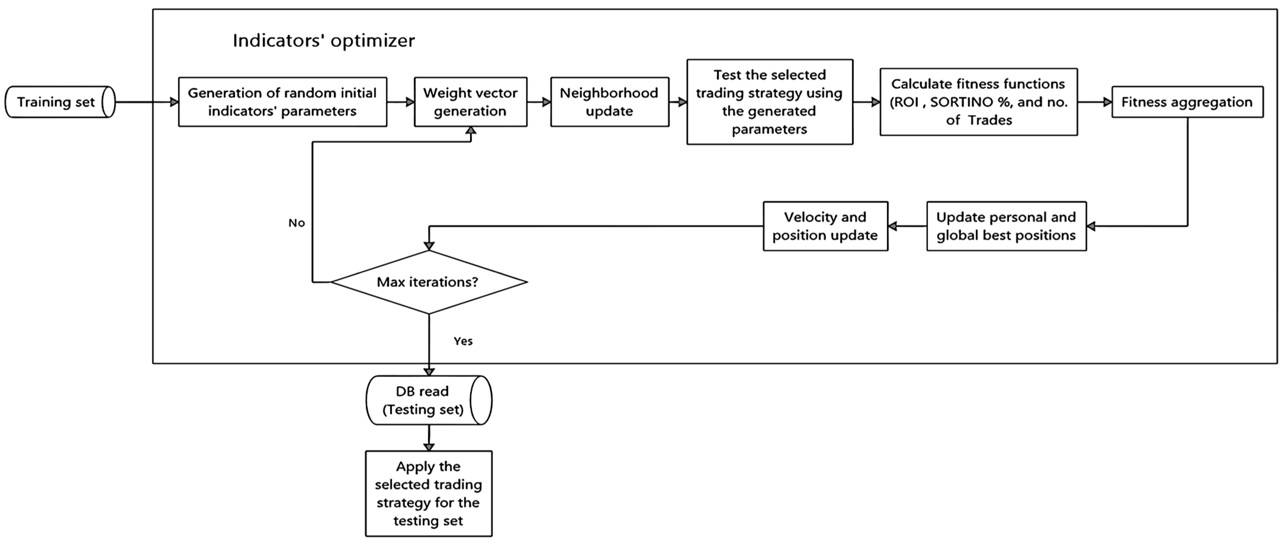
As shown in Figure 2, the algorithmic trader starts with randomly generated indicators’ parameters (particles’ positions) as well as a set of weight vectors. Applying the generated parameters to the crypto market produces a set of buy-sell signals. Such that the signals are generated based on the nature and the rules of every indicator (as shown in Section 2). These signals in turn are used to evaluate the objective functions at hand i.e., ROI, SOR, and trades.
A fitness aggregation mechanism is then applied to aggregate the objectives. Based on the aggregated value for each particle, the personal and global best positions are updated, as well as the particles’ positions and velocities as shown in Algorithm 1. The same process is repeated with the updated positions. The algorithm stops when it reaches the maximum number of iterations. Finally, it returns the non-dominated solutions found during the search process that are then applied to the testing set.
The Hybrid Weight Generation Mechanism
As previously mentioned, the weight assignment mechanism is one of the main factors that affect the MOEA/D search process. Identical or poorly distributed weight vectors lead to poor solutions that are unable to cover the entire PF [21,64]. The weight vector generation approaches can be classified into systematic and random weight generation.
In systematic weight generation, the weights are constructed in repeated patterns to ensure evenly distributed vectors over the PF. The systematic distribution works very well in problems with regular or continuous PF; however, its performance reduces for problems with complex or scattered PFs [65]. The other problem with systematic distribution is that it sometimes provides similar or very close vectors, which in turn leads to redundant solutions [12].
On the other hand, the random weight creation can provide a more thorough exploration of the search space since it generates vectors that are not necessarily equally distributed across the PF. This in turn provides some unique and diverse solutions since it creates vectors that are dissimilar to one another. The problem with random weight generation is that there is no guarantee that the generated vectors could represent the entire PF [12]. In real-world problems, the search complexity increases as the PF is scattered and hardly covered in most cases. In such a scenario, a Pareto solution set to a challenging subproblem cannot be located through a simple search. To handle this problem, a new hybrid weight assignment mechanism has been proposed.
The proposed strategy merges both the systematic and random weight assignment approaches in order to utilize the advantages of both of them in a single algorithm. The proposed methodology allows to hit different random areas in the search space while maintaining the systematic distribution mechanism.
As shown by Algorithm 2, the total number of subproblems is divided into two partitions. In the first partition, the weights are systematically generated once at equal distances across the PF, while in the second partition, they are randomly generated during each iteration.
| Algorithm 2: Hybrid weight generation algorithm |
Inputs:
Steps:
|
This process affects the neighborhood of each particle in the search space. Instead of having the same neighboring solutions during the search process, the neighbors are dynamically changed during each iteration, which in turn adds some more experience to the particles. The random assignment used here helps explore different areas that could hardly be reached using the systematic distribution alone, which aims at enhancing both convergence and diversity. In our experiments, the number of weight vectors that are systematically generated is set to 80% of the total number of SPs, while the rest of the weight vectors (20%) are randomly generated.
5. Results
The optimized algorithmic trading strategy is applied to Litecoin (LTC). The algorithm is trained first on the training data set, and then the set of the obtained optimized parameters is applied to the testing set. As mentioned before, the training and testing sets were selected in order to evaluate the performance of the proposed strategy during the COVID-19 pandemic. The cryptocurrency historical data used in this research is from CoinMarketCap and Yahoo Finance. The algorithmic trader is publicly available at https://github.com/SherinOmran/CryptoMarket.git (accessed on 23 September 2023).
5.1. Evaluation Metrics
The evaluation metric is an indicator or a measure of the quality of the generated solutions. There are various kinds of metrics to evaluate the MOO algorithms, each of which is used to evaluate different criteria [66]. Among the most important evaluation criteria are convergence, diversity, and statistical measurements. Different metrics have been found that evaluate either one or more criteria simultaneously. Three different indicators were used in this study: the Generational Distance (GD), the Hypervolume (HV), and the Average Fitness Value (AFV).
The GD is a convergence indicator that is used to measure the distance between the obtained non-dominated solutions (the obtained, also called the approximated PF) and the true PF [66,67]. Since the true PF is not known in real-world problems, a reference set that is obtained from the collection of the final non-dominated solution set among the approximated PFs found by all the considered search algorithms can be used instead. As a measure of how close the obtained solution set is to the true PF or the reference set, the lowest GD value is the best, and vice versa.
The HV indicator is a measure of both diversity and convergence. The HV quantifies the N-dimensional volume of the objective space area bounded by the approximated PF (y) and a dominated reference point (r) [66]. Higher values of the HV indicate a larger dominated area by the obtained approximated PF, so a higher HV is always preferred.
The AFV of each objective is calculated as the average of the fitness of the non-dominated solutions found during independent runs. Such that the total number of solutions are the number of non-dominated solutions found during each run multiplied by . However, the number of non-dominated solutions is not necessarily the same during each run. The results are available at https://drive.google.com/drive/folders/1V-bBCcs2L9XoOrXasHa4aowTf0oj0C8a (accessed on 23 September 2023).
5.2. Benchmark Problems
The proposed algorithm is first tested on three benchmark minimization problems with different PF shapes, i.e., ZDT2 [21], ZDT3 [21], and Viennet [68]. Such that, ZDT2 and ZDT3 are bi-objective problems, whereas the Viennet problem is a tri-objective problem.
To evaluate the performance of the hybrid assignment mechanism (MOPSO/D-Hyb), the proposed algorithm is compared against both Pareto-dominance-based algorithms, i.e., SPEA2 [69] and decomposition-based algorithms, i.e., the original MOEA/D and MOPSO/D with systematic weight distribution (MOPSO/D-Sys). For fair comparison and to evaluate the effect of the hybrid strategy clearly without any external improvements (specifically the normalization effect), all the three decomposition-based algorithms are implemented using the non-normalized WTCH aggregation function. In this case, all the algorithm steps are the same as mentioned, except step 2.1 in Algorithm 1, which will be replaced with Equation (11).
The parameter settings for the bi-objectives benchmark problems are as follows: The number of SPs for each of the algorithms is set to 250, the number of iterations is 100, the neighborhood size (T) is 20, a uniform mutation with a mutation rate of 0.25 (in this case, only one randomly selected decision variable is changed with each SP according to the mutation probability). The inertia weight is 0.98, and both and are set to 2. For the original MOEA/D, a blend crossover with a crossover rate of 1 is used, whereas the other parameters are the same. The number of SPs for the Viennet problem is set to 435 with 150 iterations while the rest of the parameters are kept the same as the other problems.
The results of the benchmark problems are evaluated based on the GD and HV obtained by each algorithm on each benchmark problem, such that the reported results are the best and average values over 20 independent runs.
Table 1 shows the best and average GD and HV as well as their standard deviations (STD) obtained by each algorithm for ZDT2, ZDT3, and the Viennet benchmark problems in sequence. The best result in each case is highlighted in bold.
As seen from the table, the original MOEA/D always had the least performance in terms of all the evaluation metrics at hand. Although SPEA2 showed the best obtainable GD in the Viennet problem, it could not efficiently cover the whole PF as shown by the associated HV values. In ZDT3 problem, it showed a good approximation to the true PF as it provided the second-best average values for both GD and HV, whereas it provided the lowest performance in the ZDT2 problem for all metrics. It can be seen that the MOPSO/D-Sys could provide good performance in the continuous optimization problem, i.e., ZDT2, as it provided the least average GD and could efficiently cover the whole PF. However, the STD of the GDs of the provided solutions is not the best. For the other benchmarks, the performance of MOPSO/D-Sys reduces in terms of both GD and HV, and the performance is not always stable, as can be seen through the STD of both metrics. On the other hand, the hybrid weight generation MOPSO/D-Hyb provided the best performance in problems with scattered PFs, i.e., ZDT3, and Viennet. MOPSO/D-Hyb has the best coverage of the PF, having the highest HVs, and the closest solution set to the true PF as it has the least GD. For the continuous problem, i.e., ZDT2, it could always cover the whole PF, giving equal best and average HV with MOPSO/D-Sys. Although the hybrid distribution strategy could not find the best average GD, it could find the best obtainable GD. The hybrid distribution strategy provided the least STD over all the test instances, which emphasizes its stability during different runs.
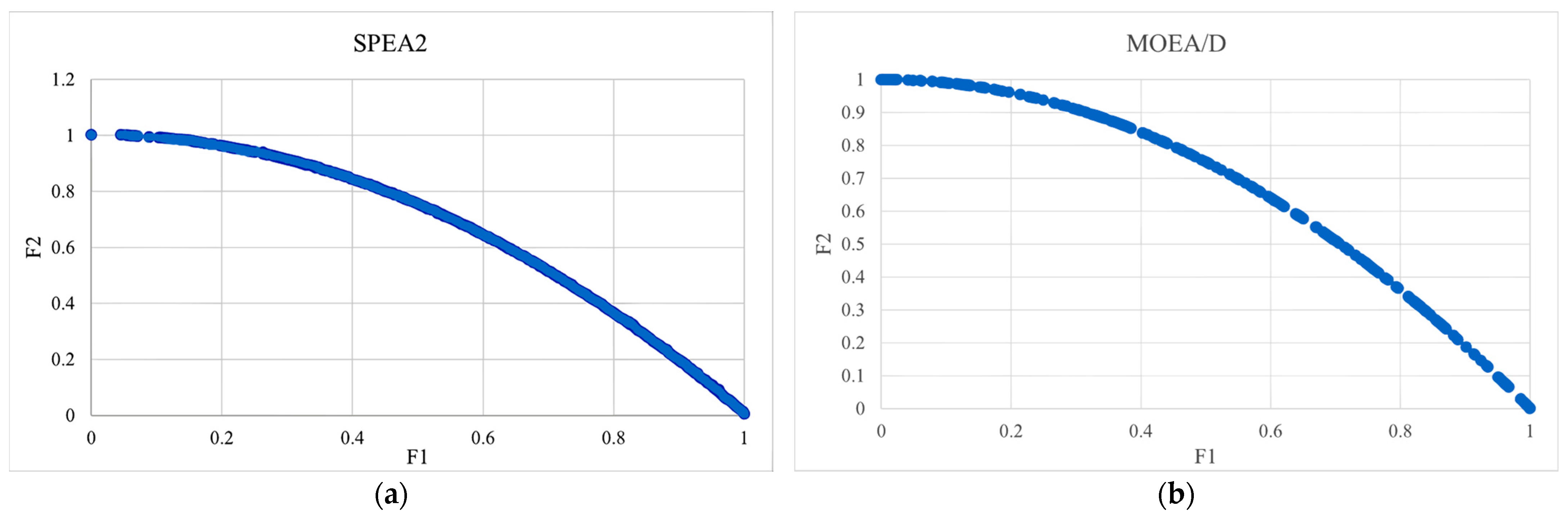
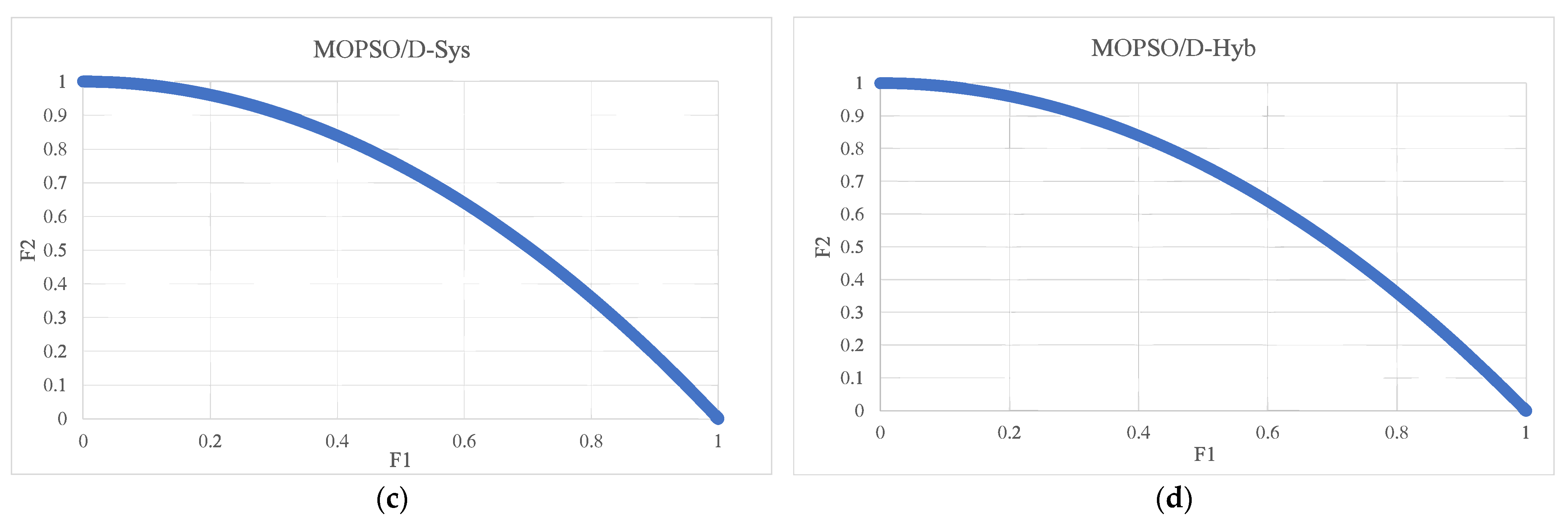
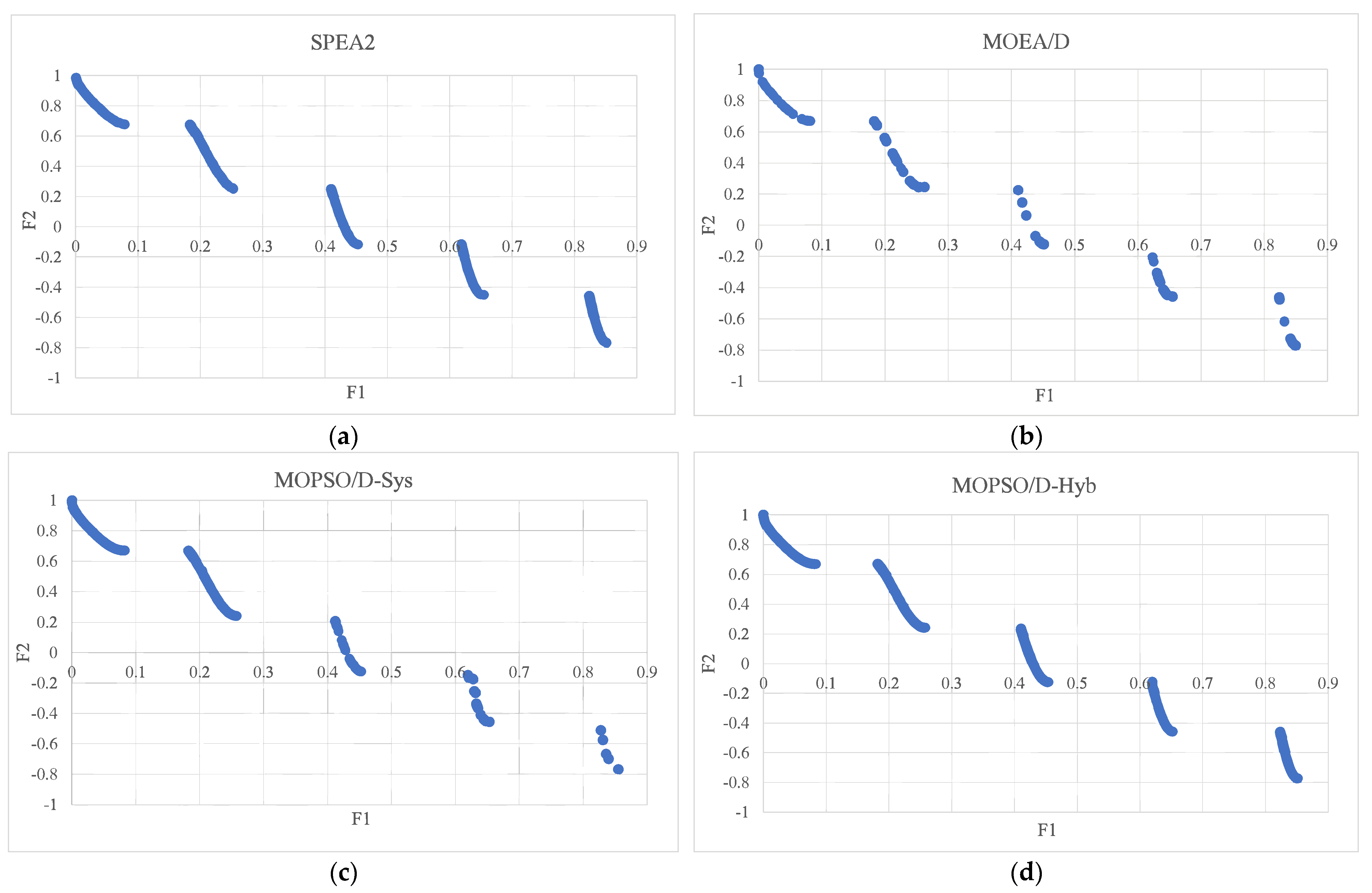
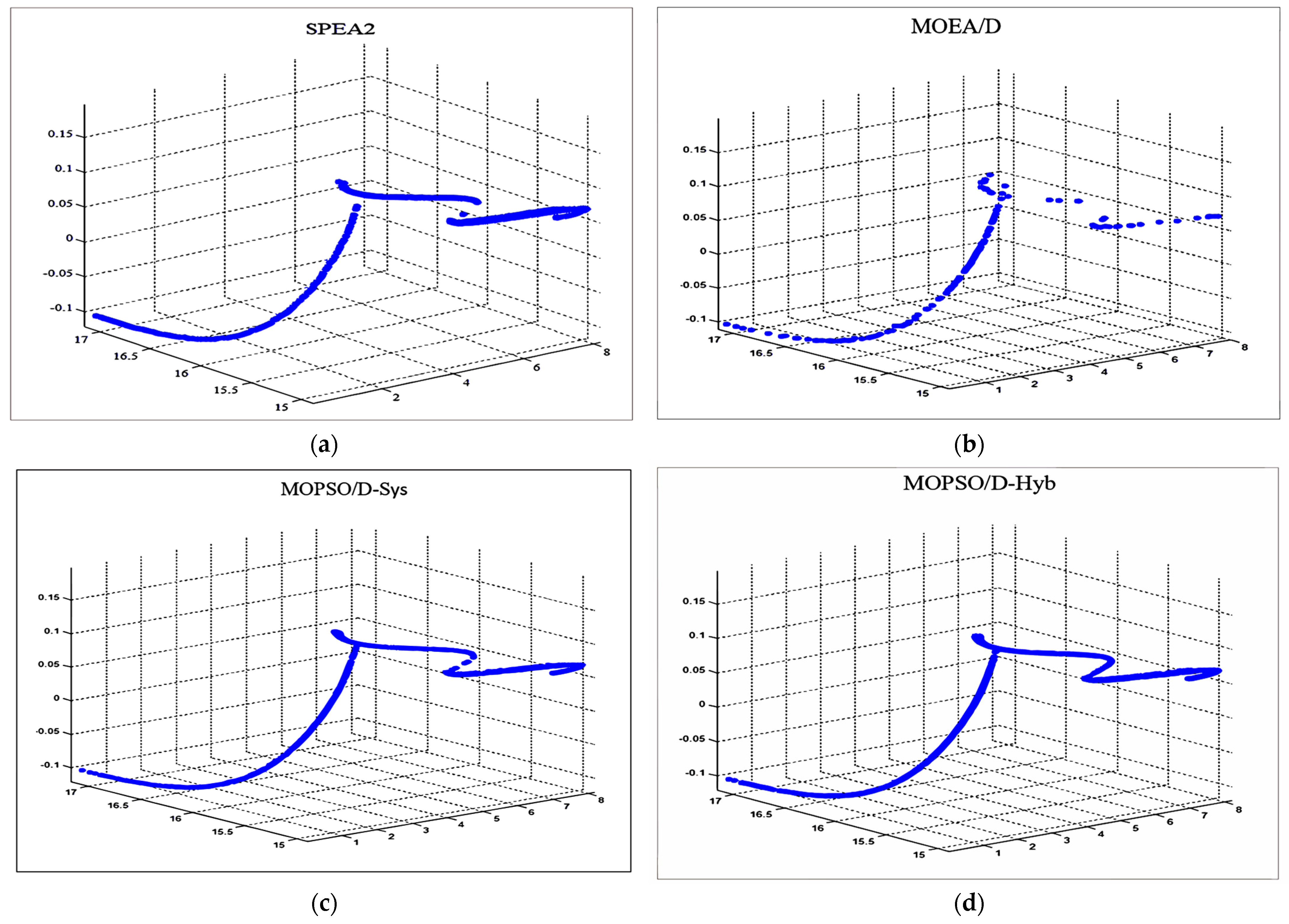
For more clarity, the PF solutions with the median GD for each algorithm over the different problems are presented in the following figures, such that Figure 3 shows the PFs obtained by the algorithms under study for the ZDT2 problem. Figure 4 presents the PFs for the ZDT3 problem, whereas Figure 5 shows the obtained PFs for the Viennet optimization problem. It can be seen from the figures that the hybrid weight generation could maintain the best distribution of solutions along the entire PFs for all the test instances. MOPSO/D-Sys showed the best distribution of solutions for only ZDT2. The MOEA/D algorithm always provided the least performance and could not efficiently cover the entire PFs for all the test instances. For SPEA2, it could efficiently cover the PF only in the ZDT3 problem.
5.3. The Algorithmic Trader Experimental Results
As seen above, the hybrid weight distribution methodology could provide the best results for the benchmark problems. For the algorithmic trader optimizer problem, four algorithms are used in comparison. The original MOEA/D is tested against the MOPSO/D using the normalized WTCH scalarization (N-WTCH). The other two are MOPSO/D using the proposed normalized AWTCH presented in Equation (14); one uses the systematic weight distribution denoted as (N-AWTCH-Sys), whereas the other uses the hybrid weight distribution denoted as (N-AWTCH-Hyb).
The parameter settings are as follows: The swarm size m = 351, where the organizing parameter H = 25. For the N-AWTCH-Hyb, the swarm is divided into two partitions; the first partition used for systematic weight distribution is chosen with H = 22, which generates 276 SPs, while the other partition size is 75 to keep the same total number of SPs (351 as the other algorithms). The maximum number of iterations is 200. The augmentation parameter is set to 0.05. A small neighborhood size T = 20 is selected to maintain the solutions’ diversity. For PSO parameters, the inertia parameter is 0.98, whereas the constant accelerators and are set to 2 and the mutation rate is 0.15. For MOEA/D, the crossover rate is 1 and the mutation rate is 0.15. The indicators’ parameters ranges are as follows: The number of days for any of the indicators ranges from 3 to 200 days. The St-RSI over-bought level , whereas the over-sold level . The S-RoC over-bought and over-sold levels range from 0 to 20% above and below the center line.
As mentioned before, the algorithms are evaluated based on the GD, the HV, and the AFVs found by each algorithm over five independent runs.
Table 2 shows the best and average HV and GD values obtained by optimizing the four trading strategies, i.e., L-WMA, St-RSI, S-ROC, and BB, using the four counterpart algorithms. The best results in each case are highlighted in bold. The results show clearly that the proposed N-AWTCH could outperform both the original MOEA/D and the N-WTCH in terms of the distribution of solutions and the distance to the true PF. Adding the hybrid distribution to the N-AWTCH could further improve the accuracy of the obtained results for most of the test instances.
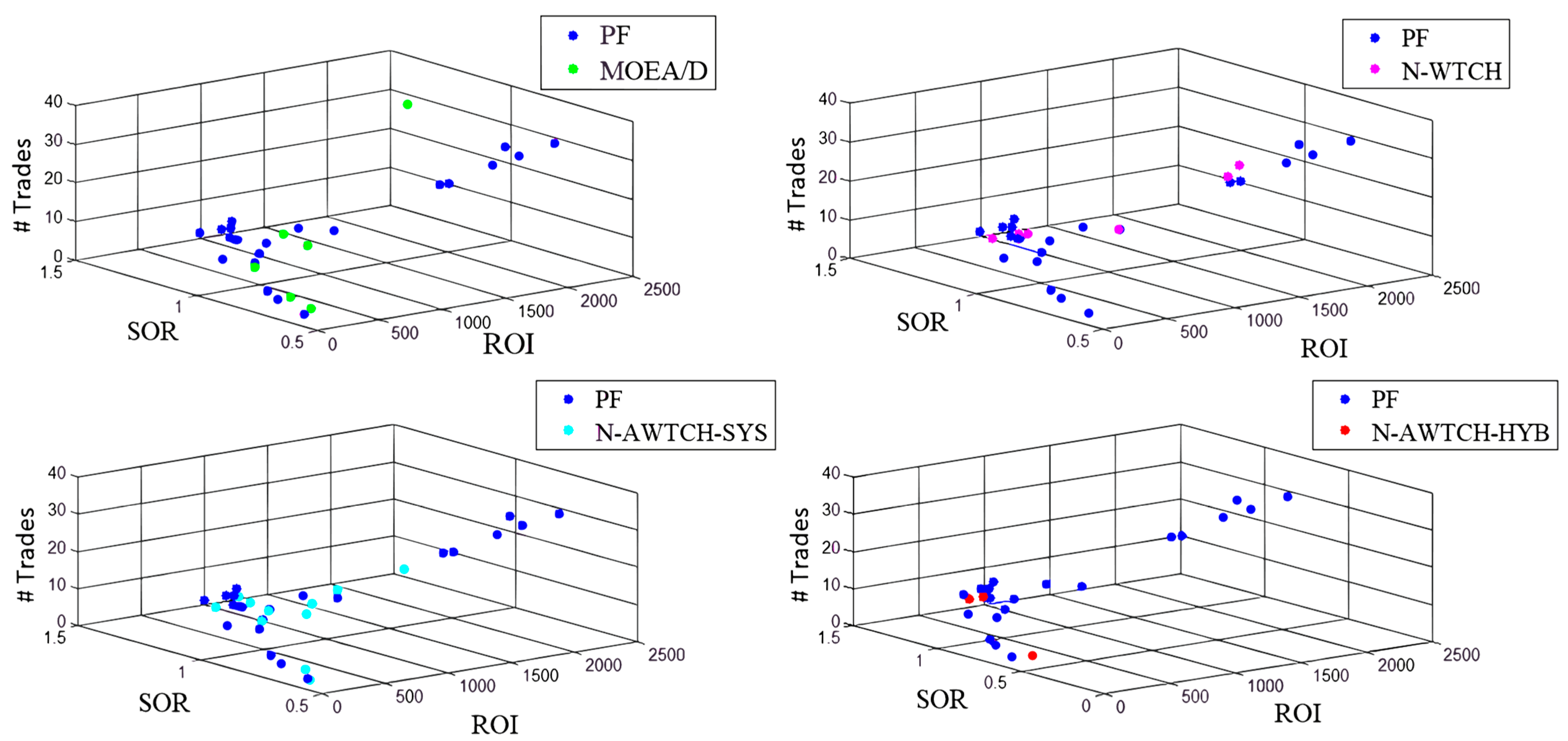
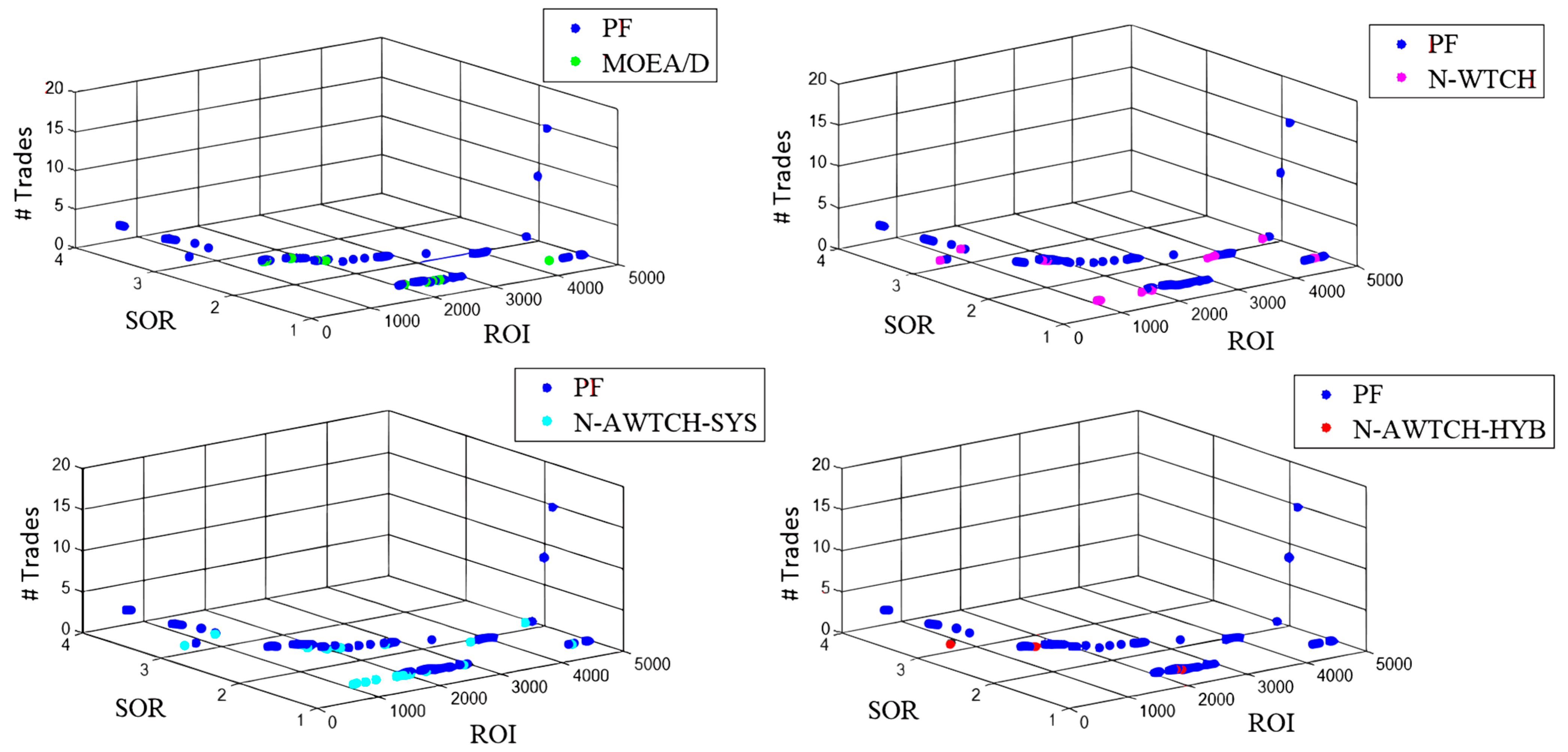
Figure 6 and Figure 7 show the approximated PFs obtained by optimizing the L-WMA and the St-RSI indicators in sequence. The two indicators, i.e., L-WMA and St-RSI, are selected as samples to figure out the shape of the true PF for each case and the distribution of the results. The figures show a comparison between the approximated PF solutions obtained by each of the algorithms under study and the true PF, such that the approximated PFs shown are the final solutions obtained from the run with the least GD. As seen from the figures, the shape of the true PFs is different for each test instance; however, they are all scattered.
To evaluate the results obtained by each algorithm in accordance with the indicators using their standard parameters, the AFVs for the final set of non-dominated solutions obtained by each algorithm are calculated. The non-dominated solutions are a set of vectors, where each vector has three components, one for each objective, i.e., ROI, SOR, and number of trades. The AFV is calculated by averaging the objectives of the non-dominated PF solutions over a set of five independent runs for each test instance in training.
During testing, the solutions obtained by each algorithm are re-evaluated, and the performance is averaged in the same way as in the training period. As is the case of all MOO problems, there are always tradeoffs between the objectives, so in order to compare the overall performance of each of the algorithms with the indicators’ standard parameters, each of the competitors is given a rank associated with each objective. The best value is given a rank of 1, and the second best is given a rank of 2, etc., while the worst value is assigned a rank of 5. The comparison includes the four counterpart algorithms and the indicator′s performance using their standard parameters.
Table 3 and Table 4 show a comparison of the AFVs by each algorithm for each trading strategy, i.e., TI, during the training and testing periods in sequence. The results reported as standard are the values of the objectives obtained by trading using the standard parameters of each indicator.
For example, as shown in Table 3, applying the L-WMA indicator using the crossovers between the 20–50 days L-WMAs to generate the trading signals, i.e., buy and sell, gives a set of 10 trades (each buy-sell pair is considered a single trade) with an overall ROI of 2677.46% and a SOR of 0.97, such that SOR is the measure of risk. By applying the same parameters to the L-WMA indicator during testing (Table 4), the overall ROI is 266.81% with a SOR of 0.78 over 10 trades.
The best AFV obtained in each case is highlighted in bold and given a rank of 1. As mentioned before, the optimization problem at hand has three objectives. Two of them are to be maximized, i.e., ROI and SOR, whereas the third objective is to be minimized, i.e., number of trades. So that the highest ROI values, SOR, and the minimum number of trades are highlighted in each case.
As seen from Table 4, the average number of trades is less than one in some cases. That is because some of the obtained parameters did not generate trading signals during testing. In such a case, values less than one cannot be considered the best values. To handle this limitation, the algorithm that provided an average number of trades less than one is assigned the same rank as the ROI.
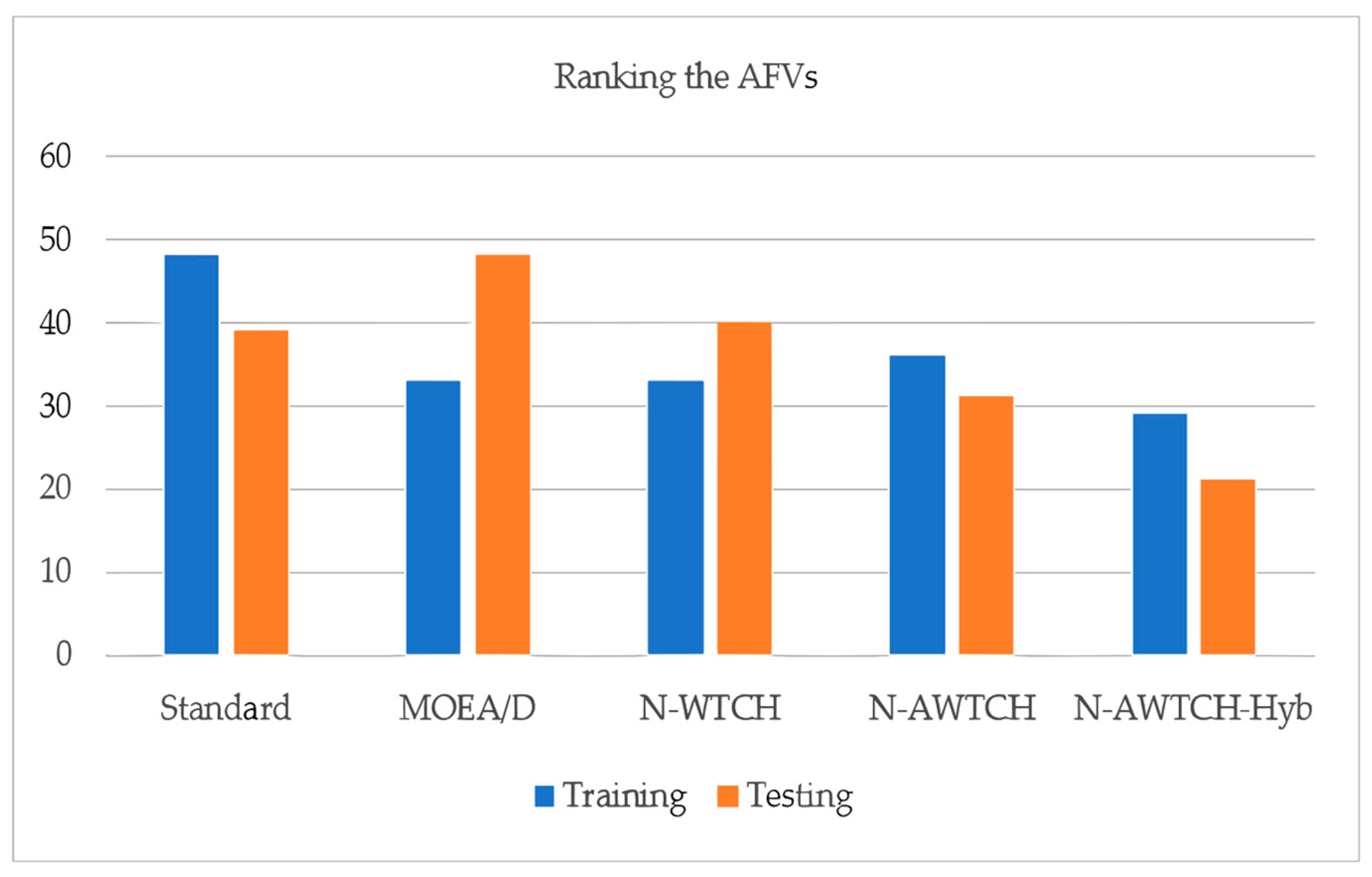
To evaluate the results presented in the last tables, the ranks obtained by each algorithm are summed, and the algorithm with the least summation of ranks is preferred. The summation of the ranks obtained by each algorithm during both training and testing is clarified in Figure 8.
For example, by going back to Table 3, the sum of ranks for MOEA/D during training is 33. The ranks assigned to the MOEA/D algorithm for L-WMA (5, 2, 1) for ROI, SOR, and number of trades in sequence, the ranks for St-RSI are (4, 4, 4), the ranks assigned to S-RoC are (4, 1, 1), and the ranks for BB are (4, 1, 2). The summation of the ranks obtained by each case gives an overall rank of 33, and so on for the rest of the competitive algorithms and the standard trading strategies.
It is obvious from the figure that N-AWTCH-Hyb has the best ranking during both training and testing, followed by both MOEA/D and N-WTCH during training, and N-AWTCH-Sys during testing. As seen from the results, the proposed algorithm provided the best trading strategies as compared to the other counterparts.
6. Discussion
Finding the best trading strategies is a great challenge for traders, as they always aim to find the most profitable strategy with the minimum level of risk. The crypto market is one of the most challenging markets due to the sudden daily fluctuations in prices. This research aims at finding the optimal parameters for four different trading strategies (also called TIs), i.e., L-WMA, St-RSI, S-RoC, and BB. The proposed algorithm is applied for one of the highest volume cryptocurrencies, i.e., LTC, using decomposition-based strategies, taking into consideration three conflicting objectives, i.e., ROI, SOR, and number of trades. The first two objectives are to be maximized whereas the last one is to be minimized.
As seen from the figures, the true PF shapes for our test instances are complex and scattered, with no definite shape. In this research, a MOPSO/D algorithm is proposed with a hybrid weight generation strategy that merges both systematic and random weight generations in order to handle the complexity of the PFs for the problem at hand.
In general, weight vector generation is one of the main factors that affect the performance of decomposition-based algorithms, as these weights are used to determine the neighborhood of each SP, which is important for recombination purposes and the generation of new solutions. Zhang [21] suggested that the recombination be performed within the same neighborhood; however, some argued that this is not efficient for more complex problems and suggested recombination with solutions from different neighborhoods instead [69].
With the proposed hybrid weight generation strategy, the recombination process (represented by position update) is performed with the help of the information gained from the same neighborhood; however, some particles (specifically, the particles with random weight generation) move through different neighborhoods over the iterations. This in turn improves the experience of the particles over time and ensures both diversity and convergence.
To test the performance of the proposed algorithm before applying it to our real-world problem, it was tested on three different benchmark problems with different PF shapes, i.e., ZDT2, ZDT3, and Viennet, such that ZDT2 has a concave continuous PF, whereas ZDT3 and Viennet have more complex and discontinuous PFs. It was proved that the proposed MOPSO/D-Hyb could overcome the performance of both the original MOEA/D and MOPSO/D using the systematic weight generation (MOPSO/D-Sys) in terms of all the evaluation metrics for the test instances at hand except for the average GD for ZDT2 problem, which was slightly worse than MOPSO/D-Sys. This means that the proposed algorithm could efficiently cover the true PF for complex problems, with discontinuity covering all the scattered partitions.
As the objectives of our real-world optimization problem have a very wide and extensively different range of variables, there was a need for an objective normalization process.
In this research, a new linearly normalized AWTCH (N-AWTCH) scalarization method has been proposed. The proposed algorithm was implemented in both systematic (N-AWTCH-Sys) and hybrid (N-AWTCH-Hyb) weight distribution strategies and is compared against the MOPSO/D using normalized WTH (denoted as N-WTCH) and the original MOEA/D.
As seen from Table 2, the proposed normalization method N-AWTCH-Sys could obtain better solutions in terms of GD and HV as compared to the original MOEA/D and N-WTCH, where it could outperform them in three out of the four test instances in terms of the average GD and two test instances in terms of the average HV.
As compared to the hybrid weight distribution strategy, the N-AWTCH-Hyb could further improve the performance of the N-AWTCH-Sys in terms of both GD and HV obtaining the best results in three out of the four test instances as compared to the other counterparts.
As noticed from the figures Figure 6 and Figure 7, the number of true PF points is limited that is due to many reasons. Among the factors that affect the number of true PF points is the relationship between the objectives, such that the objectives at hand are highly skewed. The second reason is the effect of the market changes during the period under study (i.e., the COVID-19 pandemic), such that a large number of parameter combinations are found to be non-sensitive to the market changes, generating either non-profitable trades or no trades. Moreover, some parameter combinations are found to generate the same trading signals.
To examine the performance of the proposed algorithm in terms of the efficiency of the generated trading strategies, the AFVs of the algorithms under study as well as the indicators using their standard parameters are calculated and ranked, such that the lowest rank is the best and the highest is the worst. It was found that the proposed algorithm (N-AWTCH-Hyb) obtains the best summation of ranks during both the training and testing periods.
By examining the ranking of the proposed algorithm in terms of each objective individually, we can find that it has the best ranking in terms of both ROI and SOR during both training and testing periods. In terms of the number of trades, it was found that the proposed algorithm sometimes provides a high number of trades during training; however, these trades are profitable. During testing, it could also provide the best ranking in terms of the number of trades.
7. Conclusions
The crypto market is extremely risky and volatile, which makes it hard to predict. An optimized algorithmic trading approach using four independent technical indicators (i.e., L-WMA, St-RSI, S-RoC, and BB) has been proposed, taking into consideration the trade-offs between different objectives. A Normalized MOPSO/D has been used to optimize the algorithmic trading over three different objectives: ROI, SOR, and number of trades. The normalization mechanism is applied for the Augmented Weighted-Tchebycheff (A-WTCH) scalarization function (N-AWTCH). As real-world optimization, problems always have complex PFs that are hardly covered with the regular weight generation strategy of the original decomposition approach, a hybrid weight distribution strategy is proposed that combines both systematic and random weight generations. In this context, a single grid of weight vectors is generated and partitioned such that the first partition is assigned constant and equally distant weight vectors that are generated once, whereas the other partition is randomly generated during each iteration. To evaluate the performance of the hybrid weight distribution strategy, it was first applied to some benchmark problems with different PF shapes and tested against the original MOEA/D and MOPSO/D with systematic weight distribution. The proposed algorithm was found to optimize the PF finding the best Generational Distance (GD) and Hyper Volume (HV) for problems with irregular PF shapes (i.e., noncontinuous and degenerated), which emphasizes the ability of the proposed weight generation strategy to handle complex PFs.
The proposed algorithm combining the N-AWTCH aggregation function as well as the hybrid weight distribution (N-AWTCH-Hyb) is applied to the real-world problem at hand and is compared against the N-AWTCH using systematic weight distribution (N-AWTCH-Sys), the normalized version of the WTCH scalarization (N-WTCH), the original MOEA/D, as well as the indicators with their standard parameters. Three different evaluation criteria have been taken into account: the GD, the HV, and the Average Fitness Values (AFV). The proposed approaches were tested on Litecoin, across training and testing sets. The COVID-19 outbreak has been taken into consideration such that the training period is the pre-pandemic period, whereas the testing period is considered the pandemic period.
Results showed that the proposed N-AWTCH-Hyb outperformed the other counterpart algorithms in 75% of the test instances in terms of both convergence and diversity indicators (i.e., GD and HV). In terms of the AFVs, the proposed strategy provided the best ranking as compared to all the competitive algorithms as well as the indicators with their standard parameters. Although there were extreme market changes during both training and testing due to the outbreak effect, the optimized trading strategy using the proposed algorithm revealed its stability over the other counterparts during both training and testing periods (which is the main challenge).
Author Contributions
Conceptualization, A.A.A.Y. and W.H.E.-B.; data curation, S.M.O.; formal analysis, S.M.O. and A.A.A.Y.; investigation, W.H.E.-B.; methodology, S.M.O.; supervision, A.A.A.Y.; validation, W.H.E.-B.; writing—original draft, S.M.O.; writing—review and editing, A.A.A.Y. and W.H.E.-B. All authors have read and agreed to the published version of the manuscript.
Funding
This research received no external funding.
Informed Consent Statement
Informed consent is not required for this study.
Data Availability Statement
The data used in this study is publicly available on CoinMarketCap.
Conflicts of Interest
All authors declare that they have no conflict of interest.
References
- Daskalakis, N.; Georgitseas, P. An Introduction to Cryptocurrencies: The Crypto Market Ecosystem; Routledge: London, UK, 2020. [Google Scholar]
- Sebastião, H.; Godinho, P. Forecasting and trading cryptocurrencies with machine learning under changing market conditions. Financ. Innov. 2021, 7, 3. [Google Scholar] [CrossRef]
- Jaquart, P.; Dann, D.; Weinhardt, C. Short-term bitcoin market prediction via machine learning. J. Financ. Data Sci. 2021, 7, 45–66. [Google Scholar] [CrossRef]
- Borrageiro, G.; Firoozye, N.; Barucca, P. The Recurrent Reinforcement Learning Crypto Agent. IEEE Access 2022, 10, 38590–38599. [Google Scholar] [CrossRef]
- Gyamerah, S.A. Two-Stage Hybrid Machine Learning Model for High-Frequency Intraday Bitcoin Price Prediction Based on Technical Indicators, Variational Mode Decomposition, and Support Vector Regression. Complexity 2021, 2021, 1767708. [Google Scholar] [CrossRef]
- Carbó, J.M.; Gorjon, S. Application of Machine Learning Models and Interpretability Techniques to Identify the Determinants of the Price of Bitcoin; Working Paper No. 2215; Carbó, J.M., Gorjon, S., Eds.; IdeBanco de Espana: Madrid, Spain, 2022. [Google Scholar]
- Ammer, M.A.; Aldhyani, T.H.H. Deep Learning Algorithm to Predict Cryptocurrency Fluctuation Prices: Increasing Investment Awareness. Electronics 2022, 11, 2349. [Google Scholar] [CrossRef]
- Akila, V.; Nitin MV, S.; Prasanth, I.; Reddy, S.; Kumar, A. A Cryptocurrency Price Prediction Model using Deep Learning. E3S Web Conf. 2023, 391, 01112. [Google Scholar]
- Negi, P.; Dhawad, R.; Morris, N.C.; Agrawal, R.; Dhule, C. Cryptocurrency Price Analysis using Deep Learning. In Proceedings of the International Conference on Sustainable Computing and Smart Systems (ICSCSS), New Delhi, India, 10–12 July 2023. [Google Scholar]
- El-Berawi, A.S.; Belal, M.A.F.; Abd Ellatif, M.M. Adaptive Deep Learning based Cryptocurrency Price Fluctuation Classification. Int. J. Adv. Comput. Sci. Appl. (IJACSA) 2021, 12, 487–500. [Google Scholar] [CrossRef]
- Frajtova-Michalikova, K.; Spuchľakova, E.; Misankova, M. Portfolio Optimization. In Proceedings of the 4th World Conference on Business, Economics and Management, WCBEM, Ephesus, Turkey, 30 April–2 May 2015. [Google Scholar]
- Hrytsiuk, P.; Babych, T.; Bachyshyna, L. Cryptocurrency Portfolio Optimization Using Value-At-Risk Measure. In Proceedings of the 6th International Conference on Strategies, Models and Technologies of Economic Systems Management (SMTESM 2019), Khmelnytskyi, Ukraine, 4–6 October 2019. [Google Scholar]
- He, Y.; Aranha, C. Solving Portfolio Optimization Problems Using MOEA/D and L´evy Flight. Adv. Data Sci. Adapt. Anal. 2020, 12, 2050005. [Google Scholar] [CrossRef]
- Joemon, B.; Ghazanfar, M.A.; Azam, M.A.; Jhanjhi, N.Z.; Khan, A.A. Novel heuristics for Stock portfolio optimization using machine learning and Modern Portfolio Theory. In Proceedings of the International Conference on Business Analytics for Technology and Security (ICBATS), Dubai, United Arab Emirates, 7–8 March 2023. [Google Scholar]
- Lorenzo, L.; Arroyo, J. Online risk-based portfolio allocation on subsets of crypto assets applying a prototype-based clustering algorithm. Financ. Innov. 2023, 9, 25. [Google Scholar] [CrossRef]
- Karahan, Ç.; Öğüdücü, Ş.G. Cryptocurrency Trading based on Heuristic Guided Approach with Feature Engineering. In Proceedings of the International Conference on Data Science and Its Applications (ICoDSA), Bandung, Indonesia, 6–7 July 2022. [Google Scholar]
- Leung, M.-F.; Chan, L.; Hung, W.-C.; Tsoi, S.-F.; Lam, C.-H.; Cheng, Y.-H. An Intelligent System for Trading Signal of Cryptocurrency Based on Market Tweets Sentiments. FinTech 2023, 2, 153–169. [Google Scholar] [CrossRef]
- Koker, T.E.; Koutmos, D. Cryptocurrency Trading Using Machine Learning. Risk Financ. Manag. 2020, 13, 178. [Google Scholar] [CrossRef]
- Deb, K. Multi-Objective Optimization Using Evolutionary Algorithms; John Wiley & Sons, Inc.: New York, NY, USA, 2001. [Google Scholar]
- Omran, S.M.; El-Behaidy, W.H.; Youssif, A.A.A. Decomposition Based Multi-objectives Evolutionary Algorithms Challenges and Circumvention. Adv. Intell. Syst. Comput. 2020, 1229, 82–93. [Google Scholar]
- Zhang, Q.; Li, H. MOEA/D: A Multiobjective Evolutionary Algorithm Based on Decomposition. IEEE Trans. Evol. Comput. 2007, 11, 712–731. [Google Scholar] [CrossRef]
- Bui, L.T.; Alam, S. Multi Objective Optimization in Computational Intelligence: Theory and Practice, Hershey; IGI Global: New York, NY, USA, 2008. [Google Scholar]
- Jiang, S.; Cai, Z.; Zhang, J.; Ong, Y.-S. Multiobjective Optimization by Decomposition with Pareto-adaptive Weight Vectors. In Proceedings of the Seventh International Conference on Natural Computation, Shanghai, China, 26–28 July 2011. [Google Scholar]
- Guo, X.; Wang, X.; Wei, Z. MOEA/D with Adaptive Weight Vector Design. In Proceedings of the 11th International Conference on Computational Intelligence and Security, Shenzhen, China, 19–20 December 2015. [Google Scholar]
- Wu, M.; Kwong, S.; Jia, Y.; Li, K.; Zhang, Q. Adaptive weights generation for decomposition-based multi-objective optimization using Gaussian process regression. In Proceedings of the GECCO’17 Genetic and Evolutionary Computation Conference, Berlin, Germany, 15–19 July 2017. [Google Scholar]
- Farias, L.R.C.D.; Braga, P.H.M.; Bassani, H.F.; Araújo, A.F.R. MOEA/D with Uniformly Randomly Adaptive Weights. In Proceedings of the GECCO’18, Kyoto, Japan, 15–18 July 2018. [Google Scholar]
- Zheng, R.; Wang, Z. A Generalized Scalarization Method for Evolutionary Multi-Objective Optimization. In Proceedings of the Thirty-Seventh AAAI Conference on Artificial Intelligence (AAAI-23), Washington, DC, USA, 7–14 February 2023. [Google Scholar]
- Jiang, S.; Yang, S.; Wang, Y.; Liu, X. Scalarizing Functions in Decomposition-Based Multiobjective Evolutionary Algorithms. IEEE Trans. Evol. Comput. 2018, 22, 296–313. [Google Scholar] [CrossRef]
- Rodriguez, A.V.B.; Coello, C.A.C. Designing Scalarizing Functions Using Grammatical Evolution. In Proceedings of the GECCO’23, Lisbon, Portugal, 15–19 July 2023. [Google Scholar]
- Ishibuchi, H.; Sakane, Y.; Sakane, Y.; Sakane, Y. Simultaneous Use of Different Scalarizing Functions in MOEA/D. In Proceedings of the GECCO’10, Portland, OR, USA, 7–11 July 2010. [Google Scholar]
- Pescador-Rojas, M.; Coello, C.A.C. Collaborative and Adaptive Strategies of Different Scalarizing Functions in MOEA/D. In Proceedings of the IEEE Congress on Evolutionary Computation (CEC), Rio de Janeiro, Brazil, 8–13 July 2018. [Google Scholar]
- Castro, O.R.; Santana, R.; Lozano, J.A.; Pozo, A. Combining CMA-ES and MOEA/DD for many-objective optimization. In Proceedings of the IEEE Congress on Evolutionary Computation (CEC), San Sebastian, Spain, 5–8 June 2017. [Google Scholar]
- Ke, L.; Zhang, Q.; Member, S.; Battiti, R. MOEA/D-ACO: A Multiobjective Evolutionary Algorithm Using Decomposition and Ant Colony. IEEE Trans. Cybern. 2013, 43, 1845–1859. [Google Scholar] [CrossRef]
- Li, H.; Zhang, Q. Multiobjective Optimization Problems With Complicated Pareto Sets, MOEA/D and NSGA-II. IEEE Trans. Evol. Comput. 2009, 13, 284–302. [Google Scholar] [CrossRef]
- Jiang, S.; Yang, S. An Improved Multiobjective Optimization Evolutionary Algorithm Based on Decomposition for Complex Pareto Fronts. IEEE Trans. Cybern. 2016, 46, 421–437. [Google Scholar] [CrossRef]
- Xu, H.; Zeng, W.; Zhang, D.; Zeng, X. MOEA/HD: A Multiobjective Evolutionary Algorithm Based on Hierarchical Decomposition. IEEE Trans. Cybern. 2019, 49, 517–526. [Google Scholar] [CrossRef]
- Xing, H.; Wang, Z.; Li, T.; Li, H. An Improved MOEA/D Algorithm for Multi-objective Multicast Routing with Network Coding. Appl. Soft Comput. 2017, 59, 88–103. [Google Scholar] [CrossRef]
- Zhang, Q.; Li, H.; Maringer, D.; Tsang, E. MOEA/D with NBI-style Tchebycheff approach for Portfolio Management. In Proceedings of the IEEE Congress on Evolutionary Computation, Barcelona, Spain, 18–23 July 2010. [Google Scholar]
- Erwin, K.; Engelbrecht, A. Meta-heuristics for portfolio optimization. In Soft Computing; Springer: Berlin/Heidelberg, Germany, 2023. [Google Scholar]
- Sarkar, S.; Das, S.; Chaudhuri, S.S. Multi-Level Thresholding with a Decomposition-based Multi-Objective Evolutionary Algorithm for Segmenting Natural and Medical Images. Appl. Soft Comput. 2017, 50, 142–157. [Google Scholar] [CrossRef]
- Hartjes, V.; Visser, S.G.; Curran, H.R. An Efficient Application of the MOEA/D Algorithm for Designing Noise Abatement Departure Trajectories. Aerospace 2017, 4, 54. [Google Scholar]
- Dachert, K.; Gorski, J.; Klamroth, K. An augmented weighted Tchebycheff method with adaptively chosen parameters for discrete bicriteria optimization problems. Comput. Oper. Res. 2012, 39, 2929–2943. [Google Scholar] [CrossRef]
- Almuqren, A.; Bukhowah, R.; Rahman, M.M.H. A Review on Risk Analysis of Cryptocurrency; Springer: Singapore, 2023. [Google Scholar]
- Lim, M.A. The Handbook of Technical Analysis; John Wiley & Sons: Singapore, 2016. [Google Scholar]
- Stanković, J.; Marković, I.; Stojanović, M. Investment Strategy Optimization Using Technical Analysis and Predictive Modeling in Emerging Markets. Procedia Econ. Financ. 2015, 19, 51–62. [Google Scholar] [CrossRef]
- Oktaba, P.; Grzywińska-Rąpca, M. Modification of technical analysis indicators and increasing the rate of return on investment. Cent. Eur. Econ. J. 2023, 1057, 148–162. [Google Scholar] [CrossRef]
- Silva, A.; Neves, R.F.; Horta, N. Portfolio Optimization Using Fundamental Indicators Based on Multi-Objective EA; Springer: Berlin/Heidelberg, Germany, 2014. [Google Scholar]
- Metaxiotis, K.; Liagkouras, K. Multiobjective Evolutionary Algorithms for Portfolio Management: A comprehensive literature review. Expert Syst. Appl. 2012, 39, 11685–11698. [Google Scholar] [CrossRef]
- Pardeshi, Y.K.; Kale, P. Technical Analysis Indicators in Stock Market Using Machine Learning: A Comparative Analysis. In Proceedings of the 12th International Conference on Computing Communication and Networking Technologies (ICCCNT), Kharagpur, India, 6–8 July 2021. [Google Scholar]
- Su, Y.; Cui, C.; Qu, H. Self-Attentive Moving Average for Time Series Prediction. Appl. Sci. 2022, 12, 3602. [Google Scholar] [CrossRef]
- Chen, Y.-H.; Chang, C.-H.; Kuo, S.-Y.; Chou, Y.-H. A Dynamic Stock Trading System Using GQTS And Moving Average in the U.S. Stock Market. In Proceedings of the IEEE International Conference on Systems, Man, and Cybernetics (SMC), Toronto, ON, Canada, 11–14 October 2020. [Google Scholar]
- García, R.M.; Ventura, E.; Sanz, R.A. Temporal optimisation of signals emitted automatically by securities exchange indicators. Cuad. Gestión 2020, 1, 61–71. [Google Scholar] [CrossRef]
- Kuo, S.-Y.; Chou, Y.-H. Building Intelligent Moving Average-Based Stock Trading System Using Metaheuristic Algorithms. IEEE Access 2021, 9, 140383–140396. [Google Scholar] [CrossRef]
- Day, M.-Y.; Cheng, Y.; Huang, P.; Ni, Y. The Profitability of Bollinger Bands Trading Bitcoin Futures. Appl. Econ. Lett. 2022, 30, 1437–1443. [Google Scholar] [CrossRef]
- Botchkarev, A. Estimating the Accuracy of the Return on Investment (ROI) Performance Evaluations. Interdiscip. J. Inf. Knowl. Manag. 2015, 10, 217–233. [Google Scholar] [CrossRef]
- Bacon, C.R. Risk-Adjusted Performance Measurement; John Wiley & Sons, Ltd.: London, UK, 2013. [Google Scholar]
- Mansour, N.; Salem, S.B. COVID-19’s Impact on the Cryptocurrency Market and the Digital Economy; IGI Global: Hershey, PA, USA, 2021. [Google Scholar]
- Ma, X.; Zhang, Q.; Tian, G.; Yang, J.; Zhu, Z. On Tchebycheff Decomposition Approaches for Multi-objective Evolutionary Optimization. IEEE Trans. Evol. Comput. 2018, 22, 226–244. [Google Scholar] [CrossRef]
- Chugh, T. Scalarizing Functions in Bayesian Multiobjective Optimization. In Proceedings of the 2020 IEEE Congress on Evolutionary Computation (CEC), Glasgow, UK, 19–24 July 2020. [Google Scholar]
- Wang, R.; Zhang, Q.; Zhang, T. Decomposition Based Algorithms Using Pareto Adaptive Scalarizing Methods. IEEE Trans. Evol. Comput. 2016, 20, 821–837. [Google Scholar] [CrossRef]
- Ishibuchi, H.; Nojima, Y.; Doi, K. On the effect of normalization in MOEA/D for multi-objective and many-objective optimization. Complex Intell. Syst. 2017, 3, 279–294. [Google Scholar] [CrossRef]
- He, L.; Ishibuchi, H.; Trivedi, A.; Wang, H.; Nan, Y.; Srinivasan, D. A Survey of Normalization Methods in Multiobjective Evolutionary Algorithms. IEEE Trans. Evol. Comput. 2021, 25, 1028–1048. [Google Scholar] [CrossRef]
- Joseph, N.P.; Ramadoss, B. A Genetic Algorithm Applying Single Point Crossover and Uniform Mutation to Minimize Uncertainty in Production Cost. World Appl. Sci. 2013, 23, 1013–1017. [Google Scholar]
- Santiago, A.; Huacuja, H.J.F.; Dorronsoro, B.; Pecero, J.E.; Santillan, C.G.; Barbosa, J.J.G.; Monterrubio, J.C.S. A Survey of Decomposition Methods for Multi-objective Optimization. Recent Advances on Hybrid Approaches for Designing Intelligent Systems. Stud. Comput. Intell. 2014, 547, 453–465. [Google Scholar]
- Chen, X.; Yin, J.; Yu, D.; Fan, X. A decomposition-based many-objective evolutionary algorithm with adaptive weight vector strategy. Appl. Soft Comput. 2022, 128, 109412. [Google Scholar] [CrossRef]
- Audet, C.; Bigeon, J.; Cartier, D.; Le Digabel, S.; Salomon, L. Performance indicators in multiobjective optimization. Eur. J. Oper. Res. 2020, 292, 397–422. [Google Scholar] [CrossRef]
- Li, M.; Chen, T. How to Evaluate Solutions in Pareto-based Search-Based Software Engineering? A Critical Review and Methodological Guidance. IEEE Trans. Softw. Eng. 2022, 48, 1771–1799. [Google Scholar] [CrossRef]
- Liu, D.; Guo, S.; Chen, X.; Shao, Q.; Ran, Q.; Song, X.; Wang, Z. A macro-evolutionary multi-objective immune algorithm with application to optimal allocation of water resources in Dongjiang River basins, South China. Stoch. Environ. Res. Risk Assess. 2012, 26, 491–507. [Google Scholar] [CrossRef]
- Zitzler, E.; Eckart, L.; Thiele, L. SPEA2: Improving the strength pareto evolutionary algorithm. In Proceedings of the Evolutionary Methods for Design, Optimization and Control with Applications to Industrial Problems, Athens, Greece, 19–21 September 2001. [Google Scholar]
Figure 1.
The crossovers between 20- and 50-days L-WMA indicator for LTC/USD trading. (The red line is for the short MA and the blue line is for the long MA, whereas the ovals show the areas of false signals) (using Tradingview.com, accessed on 8 November 2023).
Figure 1.
The crossovers between 20- and 50-days L-WMA indicator for LTC/USD trading. (The red line is for the short MA and the blue line is for the long MA, whereas the ovals show the areas of false signals) (using Tradingview.com, accessed on 8 November 2023).

Figure 2.
The proposed cryptocurrency algorithmic trader model.

Figure 3.
The set of Pareto optimal solutions found by SPEA2 (a), MOEA/D (b), MOPSO/D−Sys (c), and MOPSO/D−Hyb (d) for the ZDT2 problem.
Figure 3.
The set of Pareto optimal solutions found by SPEA2 (a), MOEA/D (b), MOPSO/D−Sys (c), and MOPSO/D−Hyb (d) for the ZDT2 problem.


Figure 4.
The set of Pareto optimal solutions found by SPEA2 (a), MOEA/D (b), MOPSO/D−Sys (c), and MOPSO/D−Hyb (d) for the ZDT3 problem.
Figure 4.
The set of Pareto optimal solutions found by SPEA2 (a), MOEA/D (b), MOPSO/D−Sys (c), and MOPSO/D−Hyb (d) for the ZDT3 problem.

Figure 5.
The set of Pareto optimal solutions found by SPEA2 (a), MOEA/D (b), MOPSO/D−Sys (c), and MOPSO/D−Hyb (d) for the Viennet problem.
Figure 5.
The set of Pareto optimal solutions found by SPEA2 (a), MOEA/D (b), MOPSO/D−Sys (c), and MOPSO/D−Hyb (d) for the Viennet problem.

Figure 6.
The approximated PF versus the true PF for L-WMA indicator optimization of each algorithm for LTC trading.
Figure 6.
The approximated PF versus the true PF for L-WMA indicator optimization of each algorithm for LTC trading.

Figure 7.
The approximated PF versus the true PF for St-RSI indicator optimization of each algorithm for LTC trading.
Figure 7.
The approximated PF versus the true PF for St-RSI indicator optimization of each algorithm for LTC trading.

Figure 8.
The summation of the ranks for each algorithm and the indicators′ standard parameters during both training and testing.
Figure 8.
The summation of the ranks for each algorithm and the indicators′ standard parameters during both training and testing.


Table 1.
The GDs and HVs obtained by each algorithm for each benchmark problem.
| GD | HV | ||||||
|---|---|---|---|---|---|---|---|
| Best | Average | STD | Best | Average | STD | ||
| ZDT2 | SPEA2 | 2.0350 × 10⁻⁴ | 2.5175 × 10⁻⁴ | 3.2318 × 10⁻⁵ | 4.4380 × 10⁻¹ | 4.4234 × 10⁻¹ | 1.0559 × 10⁻³ |
| MOEA/D | 5.7890 × 10⁻⁷ | 8.0228 × 10⁻⁷ | 9.6221 × 10⁻⁸ | 4.4620 × 10⁻¹ | 4.4480 × 10⁻¹ | 6.9510 × 10⁻⁴ | |
| MOPSO/D-Sys | 1.2353 × 10⁻⁷ | 1.5280 × 10⁻⁷ | 3.5567 × 10⁻⁸ | 4.4890 × 10⁻¹ | 4.4890 × 10⁻¹ | 5.6953 × 10⁻¹⁷ | |
| MOPSO/D-Hyb | 1.2152 × 10⁻⁷ | 1.6424 × 10⁻⁷ | 2.2852 × 10⁻⁸ | 4.4890 × 10⁻¹ | 4.4890 × 10⁻¹ | 5.6953 × 10⁻¹⁷ | |
| ZDT3 | SPEA2 | 8.7146 × 10⁻⁵ | 1.4222 × 10⁻⁴ | 7.8160 × 10⁻⁵ | 6.0030 × 10⁻¹ | 5.9765 × 10⁻¹ | 4.6254 × 10⁻¹ |
| MOEA/D | 2.9423 × 10⁻⁵ | 1.1886 × 10⁻⁴ | 9.9334 × 10⁻⁵ | 5.9890 × 10⁻¹ | 5.9646 × 10⁻¹ | 1.2709 × 10⁻³ | |
| MOPSO/D-Sys | 7.2900 × 10⁻⁶ | 4.5964 × 10⁻⁴ | 1.5465 × 10⁻³ | 6.0090 × 10⁻¹ | 5.9687 × 10⁻¹ | 1.1177 × 10⁻² | |
| MOPSO/D-Hyb | 6.9152 × 10⁻⁶ | 2.8271 × 10⁻⁵ | 2.5840 × 10⁻⁵ | 6.0160 × 10⁻¹ | 6.0020 × 10⁻¹ | 9.9233 × 10⁻⁴ | |
| Viennet | SPEA2 | 1.6463 × 10⁻⁴ | 1.9837 × 10⁻⁴ | 1.8045 × 10⁻⁵ | 6.2180 × 10⁻¹ | 6.1925 × 10⁻¹ | 9.2593 × 10⁻⁴ |
| MOEA/D | 2.688 × 10⁻⁴ | 7.7789 × 10⁻⁴ | 2.864 × 10⁴ | 6.218 × 10⁻¹ | 6.177 × 10⁻¹ | 2.520 × 10⁻³ | |
| MOPSO/D-Sys | 2.138 × 10⁻⁴ | 2.3292 × 10⁻⁴ | 1.577 × 10⁻⁵ | 6.246 × 10⁻¹ | 6.227 × 10⁻¹ | 9.080 × 10⁻⁴ | |
| MOPSO/D-Hyb | 1.745 × 10⁻⁴ | 1.9829 × 10⁻⁴ | 1.458 × 10⁻⁵ | 6.251 × 10⁻¹ | 6.233 × 10⁻¹ | 8.113 × 10⁻⁴ | |
Table 2.
The best and average GD and HV values obtained by each algorithm for the set of optimized indicators.
Table 2.
The best and average GD and HV values obtained by each algorithm for the set of optimized indicators.
| GD | HV | ||||
|---|---|---|---|---|---|
| Best | Average | Best | Average | ||
| L-WMA | MOEA/D | 1.35 × 10⁻⁴ | 9.00 × 10⁻⁴ | 4.76 × 10⁻¹ | 4.73 × 10⁻¹ |
| N-WTCH | 1.20 × 10⁻³ | 6.96 × 10⁻² | 4.45 × 10⁻¹ | 4.11 × 10⁻¹ | |
| N-AWTCH-Sys | 1.50 × 10⁻³ | 1.93 × 10⁻² | 4.76 × 10⁻¹ | 4.26 × 10⁻¹ | |
| N-AWTCH-Hyb | 9.07 × 10⁻⁵ | 2.38 × 10⁻⁴ | 4.82 × 10⁻¹ | 4.78 × 10⁻¹ | |
| St_RSI | MOEA/D | 0.344 × 101 | 0.768 × 101 | 3.75 × 10⁻¹ | 3.30 × 10⁻¹ |
| N-WTCH | 1.11 × 10⁻¹ | 1.51 × 10⁻¹ | 4.75 × 10⁻¹ | 4.68 × 10⁻¹ | |
| N-AWTCH-Sys | 8.33 × 10⁻² | 1.38 × 10⁻¹ | 4.76 × 10⁻¹ | 4.68 × 10⁻¹ | |
| N-AWTCH-Hyb | 6.17 × 10⁻² | 1.07 × 10⁻¹ | 4.88 × 10⁻¹ | 4.70 × 10⁻¹ | |
| S-RoC | MOEA/D | 2.84 × 10⁻² | 2.34 × 10⁻¹ | 5.04 × 10⁻¹ | 4.21 × 10⁻¹ |
| N-WTCH | 1.56 × 10⁻² | 7.61 × 10⁻² | 6.97 × 10⁻¹ | 6.84 × 10⁻¹ | |
| N-AWTCH-Sys | 5.50 × 10⁻³ | 1.12 × 10⁻² | 7.20 × 10⁻¹ | 7.01 × 10⁻¹ | |
| N-AWTCH-Hyb | 5.30 × 10⁻³ | 9.38 × 10⁻³ | 7.02 × 10⁻¹ | 6.96 × 10⁻¹ | |
| BB | MOEA/D | 0 | 3.92 × 10⁻³ | 6.877 × 10⁻¹ | 6.875 × 10⁻¹ |
| N-WTCH | 5.19 × 10⁻⁵ | 4.77 × 10⁻³ | 6.903 × 10⁻¹ | 6.897 × 10⁻¹ | |
| N-AWTCH-Sys | 0 | 8.80 × 10⁻⁴ | 6.897 × 10⁻¹ | 6.845 × 10⁻¹ | |
| N-AWTCH-Hyb | 0 | 2.25 × 10⁻³ | 6.903 × 10⁻¹ | 6.900 × 10⁻¹ | |
Table 3.
The AFVs obtained for each indicator using the algorithms under study during the training period for LTC.
Table 3.
The AFVs obtained for each indicator using the algorithms under study during the training period for LTC.
| Standard | MOEA/D | N-WTCH | N-AWTCH-Sys | N-AWTCH-Hyb | ||||||||||||
|---|---|---|---|---|---|---|---|---|---|---|---|---|---|---|---|---|
| ROI% | SOR | #Trades | ROI% | SOR | #Trades | ROI% | SOR | #Trades | ROI% | SOR | #Trades | ROI% | SOR | #Trades | ||
| L-WMA | AFV | 2677.46 | 0.97 | 10.00 | 1676.62 | 1.43 | 2.59 | 2101.66 | 1.42 | 3.01 | 2088.16 | 1.34 | 2.69 | 2178.14 | 1.52 | 3.33 |
| Rank | 1 | 5 | 5 | 5 | 2 | 1 | 4 | 3 | 3 | 3 | 4 | 2 | 2 | 1 | 4 | |
| St-RSI | AFV | −90.54 | -0.31 | 61.00 | 306.34 | 0.56 | 35.95 | 791.89 | 0.96 | 12.90 | 693.04 | 0.93 | 11.72 | 834.94 | 0.95 | 13.32 |
| Rank | 5 | 5 | 5 | 4 | 4 | 4 | 2 | 1 | 2 | 3 | 3 | 1 | 1 | 2 | 3 | |
| S-RoC | AFV | −71.32 | -0.21 | 4.00 | 178.67 | 25.23 | 2.48 | 411.19 | 24.26 | 7.11 | 416.39 | 18.90 | 7.18 | 403.17 | 20.01 | 6.80 |
| Rank | 5 | 5 | 2 | 4 | 1 | 1 | 2 | 2 | 4 | 1 | 4 | 5 | 3 | 3 | 3 | |
| BB | AFV | 251.470 | 8.409 | 2.000 | 306.62 | 17.68 | 2.553 | 625.95 | 12.12 | 2.59 | 651.408 | 11.94 | 2.583 | 652.253 | 11.92 | 2.583 |
| Rank | 5 | 4 | 1 | 4 | 1 | 2 | 3 | 2 | 5 | 2 | 5 | 3 | 1 | 3 | 3 | |
| Sum of ranks | 48 | 33 | 33 | 36 | 29 | |||||||||||
Table 4.
The AFVs obtained for each indicator using the algorithms under study during the testing period for LTC.
Table 4.
The AFVs obtained for each indicator using the algorithms under study during the testing period for LTC.
| Standard | MOEA/D | N-WTCH | N-AWTCH-Sys | N-AWTCH-Hyb | ||||||||||||
|---|---|---|---|---|---|---|---|---|---|---|---|---|---|---|---|---|
| ROI% | SOR | #Trades | ROI% | SOR | #Trades | ROI% | SOR | #Trades | ROI% | SOR | #Trades | ROI% | SOR | #Trades | ||
| L-WMA | AFV | 266.81 | 0.78 | 10.00 | 70.81 | 0.62 | 4.83 | 91.95 | 0.68 | 19.83 | 92.54 | 0.67 | 4.75 | 118.63 | 0.69 | 5.29 |
| Rank | 1 | 1 | 4 | 5 | 5 | 2 | 4 | 3 | 5 | 3 | 4 | 1 | 2 | 2 | 3 | |
| St-RSI | AFV | −85.02 | −0.32 | 58.00 | 43.01 | 0.09 | 40.51 | 23.43 | 0.30 | 19.83 | 25.42 | 0.31 | 18.05 | 29.5736 | 0.31 | 20.51 |
| Rank | 5 | 5 | 5 | 1 | 4 | 4 | 4 | 3 | 2 | 3 | 1 | 1 | 2 | 1 | 3 | |
| S-RoC | AFV | −30.39 | −0.07 | 5.00 | 69.74 | 2.02 | 0.91 | 144.63 | 2.10 | 5.02 | 148.74 | 2.21 | 5.09 | 150.85 | 2.26 | 4.82 |
| Rank | 5 | 5 | 2 | 4 | 4 | 4 | 3 | 3 | 3 | 2 | 2 | 5 | 1 | 1 | 1 | |
| BB | AFV | 107.87 | 3.00 | 1.00 | 106.48 | 2.07 | 3.45 | 115.28 | 2.43 | 2.59 | 117.24 | 2.44 | 2.60 | 118.83 | 2.46 | 2.50 |
| Rank | 4 | 1 | 1 | 5 | 5 | 5 | 3 | 4 | 3 | 2 | 3 | 4 | 1 | 2 | 2 | |
| Sum of ranks | 39 | 48 | 40 | 31 | 21 | |||||||||||
Disclaimer/Publisher’s Note: The statements, opinions and data contained in all publications are solely those of the individual author(s) and contributor(s) and not of MDPI and/or the editor(s). MDPI and/or the editor(s) disclaim responsibility for any injury to people or property resulting from any ideas, methods, instructions or products referred to in the content. |
© 2023 by the authors. Licensee MDPI, Basel, Switzerland. This article is an open access article distributed under the terms and conditions of the Creative Commons Attribution (CC BY) license (https://creativecommons.org/licenses/by/4.0/).
Share and Cite
MDPI and ACS Style
Omran, S.M.; El-Behaidy, W.H.; Youssif, A.A.A. Optimization of Cryptocurrency Algorithmic Trading Strategies Using the Decomposition Approach. Big Data Cogn. Comput. 2023, 7, 174. https://doi.org/10.3390/bdcc7040174
AMA Style
Omran SM, El-Behaidy WH, Youssif AAA. Optimization of Cryptocurrency Algorithmic Trading Strategies Using the Decomposition Approach. Big Data and Cognitive Computing. 2023; 7(4):174. https://doi.org/10.3390/bdcc7040174
Chicago/Turabian StyleOmran, Sherin M., Wessam H. El-Behaidy, and Aliaa A. A. Youssif. 2023. "Optimization of Cryptocurrency Algorithmic Trading Strategies Using the Decomposition Approach" Big Data and Cognitive Computing 7, no. 4: 174. https://doi.org/10.3390/bdcc7040174