
Enhancing Credit Card Fraud Detection: An Ensemble Machine Learning Approach
by
 , , and
Abdul Rehman Khalid
1, 
Nsikak Owoh
1,*,
Omair Uthmani
1,
Moses Ashawa
1,
Jude Osamor
1 and
John Adejoh
2
1
Department of Cyber Security and Networks, Glasgow Caledonian University, Glasgow G4 0BA, UK
2
Department of Software Engineering, African University of Science and Technology, Abuja 900107, Nigeria
*
Author to whom correspondence should be addressed.
Big Data Cogn. Comput. 2024, 8(1), 6; https://doi.org/10.3390/bdcc8010006
Submission received: 21 November 2023
/
Revised: 22 December 2023
/
Accepted: 28 December 2023
/
Published: 3 January 2024
Abstract
:In the era of digital advancements, the escalation of credit card fraud necessitates the development of robust and efficient fraud detection systems. This paper delves into the application of machine learning models, specifically focusing on ensemble methods, to enhance credit card fraud detection. Through an extensive review of existing literature, we identified limitations in current fraud detection technologies, including issues like data imbalance, concept drift, false positives/negatives, limited generalisability, and challenges in real-time processing. To address some of these shortcomings, we propose a novel ensemble model that integrates a Support Vector Machine (SVM), K-Nearest Neighbor (KNN), Random Forest (RF), Bagging, and Boosting classifiers. This ensemble model tackles the dataset imbalance problem associated with most credit card datasets by implementing under-sampling and the Synthetic Over-sampling Technique (SMOTE) on some machine learning algorithms. The evaluation of the model utilises a dataset comprising transaction records from European credit card holders, providing a realistic scenario for assessment. The methodology of the proposed model encompasses data pre-processing, feature engineering, model selection, and evaluation, with Google Colab computational capabilities facilitating efficient model training and testing. Comparative analysis between the proposed ensemble model, traditional machine learning methods, and individual classifiers reveals the superior performance of the ensemble in mitigating challenges associated with credit card fraud detection. Across accuracy, precision, recall, and F1-score metrics, the ensemble outperforms existing models. This paper underscores the efficacy of ensemble methods as a valuable tool in the battle against fraudulent transactions. The findings presented lay the groundwork for future advancements in the development of more resilient and adaptive fraud detection systems, which will become crucial as credit card fraud techniques continue to evolve.
1. Introduction
Fraudulent activities are on the rise within the financial sector, with an escalating trend observed in credit card fraud. The incidence of credit card fraud is expanding swiftly in tandem with the increasing daily usage of credit cards [1]. The Federal Trade Commission (FTC) report underscores the severity of the issue, noting that 2021 marked the most challenging year in history for identity theft [2]. It is crucial to note that many cases of identity theft go unreported, suggesting that the actual number may surpass the reported figures. The FTC report emphasises the need for innovative approaches to safeguard the financial well-being of both consumers and businesses.
According to the United Kingdom Finance Annual Fraud Report 2022, in 2022, over £1.2 billion was stolen through authorised and unauthorised criminal activities, equaling a staggering £2300 lost every minute. Notably, 78% of Authorised Push Payment (APP) fraud cases originated online, while 18% occurred via telecommunications channels. The banking and finance sector successfully prevented an additional £1.2 billion of unauthorised fraud, showcasing effective measures to safeguard funds [3]. One prevalent source of losses is remote purchase fraud, where fraudsters employ stolen card information for online or telephone/mail purchases, resulting in £395.7 million in losses.
Meanwhile, in the United States, reported fraud incidents surged, with the Consumer Sentinel Network recording 2.4 million fraud reports in 2022, as documented by the Federal Trade Commission’s 2022 report [2]. The total reported losses in the U.S. for 2022 reached nearly $8.8 billion, exceeding the $6.1 billion reported in 2021. Imposter scams top the list of reported fraud incidents, followed by online shopping, prizes and sweepstakes, investments, and business and job opportunities frauds. Individuals reported losses of $2.6 billion to imposters in 2022, showcasing an increase from $2.4 billion the previous year. A concerning trend involves the surge in losses attributed to business imposters, reaching $660 million in 2022, up from $196 million in 2020. Furthermore, investment scams accounted for nearly $3.8 billion in losses in 2022, more than doubling the losses reported for such scams in 2021 [2].
Various approaches, including Statistical, Machine Learning, and Deep Learning methods, are utilised for credit card fraud detection. Statistical techniques such as Regression, hypothesis testing, and clustering are applied to identify and analyse anomalies in credit card transactions. In contrast, machine learning methods leverage algorithms to detect fraudulent activity in real time by analysing historical data. Deep learning methodologies utilise neural networks to autonomously identify intricate patterns and features within complex datasets, resulting in exceptionally accurate detection of fraudulent activities.
A significant issue with credit card fraud detection is data imbalance which stems from the uneven distribution of fraudulent and non-fraudulent transactions within the dataset. This imbalance poses a risk of biased model outcomes and suboptimal fraud detection capabilities. Several studies [4,5,6] have tackled this concern through the application of machine learning techniques like data balancing, oversampling, under-sampling, and the utilisation of the synthetic minority oversampling technique (SMOTE) to manage imbalanced credit card fraud data. However, a comprehensive exploration of the effectiveness of these techniques remains lacking.
Ensemble learning models and techniques play a crucial role in credit card fraud detection. These approaches involve combining multiple individual models to create a more robust and accurate fraud detection system. Ensemble methods, such as bagging, boosting, and stacking, are commonly employed to address challenges like imbalanced datasets and to enhance overall predictive power [7]. By leveraging the strengths of diverse base models, ensemble techniques contribute to improved fraud detection performance, reducing the risk of false positives and false negatives. The adaptability and effectiveness of ensemble learning make it a valuable strategy in the continuous battle against credit card fraud [8]. Despite their success, there exists a crucial need to delve into the computational efficiency of these ensemble models.
The demand for computational efficiency in ensemble machine learning models is paramount due to its implications for real-world applicability and scalability. As these models become increasingly prevalent in finance, the ability to process large datasets swiftly and make timely predictions is crucial. Computational efficiency ensures that ensemble models can handle the complexities of intricate algorithms, intricate feature engineering, and the integration of diverse base models without compromising speed or responsiveness [8]. This metric is especially pertinent in scenarios such as credit card fraud detection, where rapid decision-making is essential for preventing financial losses. Moreover, efficient computation supports the deployment of ensemble models in resource-constrained environments, making them accessible to a broader range of applications [9].
This paper seeks to assess the overall performance, including the computational efficiency of ensemble models implementing data balancing techniques in credit card fraud detection. By addressing this gap in research, the aim is to contribute to the advancement of effective and computationally efficient strategies for mitigating fraud activities in credit card transactions. The main contributions of this paper are as follows:
- To propose an effective credit card fraud detection model that addresses the prevalent challenge of data imbalance, a major concern arising from the uneven distribution of fraudulent and non-fraudulent transactions within datasets.
- To demonstrate the computational efficiency of the proposed ensemble models, ensuring that the ensemble models can effectively handle complex algorithms, intricate feature engineering, and the integration of diverse base models without compromising speed.
- To compare the performance of various machine learning models in identifying credit card fraud, such as Support Vector Machine (SVM), K-Nearest Neighbor (KNN), Random Forest (RF), Bagging, and Boosting.
The subsequent sections of the paper are structured as follows: Section 2 reviews existing works related to credit card fraud detection, encompassing various Machine Learning and Deep Learning techniques. In Section 3, a comprehensive elucidation of the proposed model is provided. Section 4 presents experimental results, performance analyses, comparisons, and in-depth discussions. The paper is concluded in Section 5, which also includes discussions on future work pertaining to the advancement of fraud detection solutions.
2. Related Work
In this section, we examine the related literature on proposed systems and techniques for credit card fraud detection. The existing work in this field is categorised into three sections based on the technique used, i.e., Statistical methods, Machine Learning Algorithms, and Deep Learning Techniques.
2.1. Statistical Methods
Statistical approaches have been extensively employed in the identification of credit card fraud. These methods discover suspicious trends by analysing the statistical properties of transaction data [10]. Statistical models identify outlier transactions using thresholds or criteria. Popular statistical methods include descriptive statistics, hypothesis testing, and time series analysis.
Descriptive statistics, hypothesis testing, and time-series analysis detect credit card fraud. Descriptive statistics, such as mean, standard deviation, and percentiles, can help uncover abnormal transactions [11]. Hypothesis testing compares genuine and fraudulent transactions using null and alternative hypotheses and statistical tests like t-tests or chi-square tests [12]. ARIMA (AutoRegressive Integrated Moving Average) models and STL (Seasonal and Trend Decomposition using Loess) provide transaction data patterns and trends for fraud detection [13].
2.2. Deep Learning (DL) in Credit Card Fraud Detection
Deep learning teaches multi-layered neural networks hierarchical data representations. These techniques collect complex patterns and relevant attributes from high-dimensional data. They revolutionised computer vision, natural language processing, and credit card fraud detection. Convolutional Neural Networks (CNN), Long Short-Term Memory (LSTM), Multilayer Feed Forward Neural Networks (MLFF), Artificial Neural Networks (ANNs), and Recurrent Neural Networks (RNNs) are some of the deep learning algorithms.
Deep learning techniques, such as Convolutional Neural Networks (CNN), Long Short-Term Memory (LSTM), and Generative Adversarial Networks (GAN), have revolutionised various fields, including credit card fraud detection. CNNs are adept at classifying images and extracting features from temporal data, making them suitable for detecting fraud in transaction sequences. LSTM, as a recurrent neural network, excels at analysing sequential data and capturing long-term dependencies, allowing it to identify complex fraud patterns involving multiple transactions effectively. GANs, with their generator and discriminator networks, can synthesise realistic fraud patterns, enhancing the adaptability and robustness of fraud detection systems. These deep-learning approaches have significantly improved the accuracy and efficiency of credit card fraud detection [14,15,16,17].
2.3. Machine Learning (ML) in Credit Card Fraud Detection
Due to the ability to learn from data, find complex patterns, and predict credit card theft, machine learning algorithms are important in credit card fraud detection. These algorithms are supervised and unsupervised learning methods. A few of the algorithms used for CCFD (Credit Card Fraud Detection) include Logistic Regression (LR), Support Vector Machines (SVM), K-Nearest Neighbors (KNN), Naive Bayes (NB), Decision Trees (DT), Random Forest (RF), and Tree-Augmented Naive Bayes (TAN).
For credit card fraud detection, SVM, KNN, NB, DT, RF, and TAN are powerful machine learning models. SVM classifies data points using the best hyperplane [18], KNN classifies transactions based on their K-Nearest Neighbors [19], NB uses probabilistic learning to estimate class probabilities [20], DT generates decision trees for feature-based classification [20], RF combines decision trees to reduce overfitting [21], and TAN enhances NB with a tree-like dependency structure to capture feature correlations [22]. These models offer diverse approaches to identifying and preventing fraudulent transactions, contributing to robust fraud detection systems. Credit card fraud detection algorithms have pros and downsides. When choosing an algorithm for an application, dataset size, feature space, processing needs, interpretability, and fraud must be considered.
Several researchers have highlighted the route to improved fraud prevention and detection in this comprehensive analysis of credit card fraud detection with machine learning. In [23], Prasad Chowdary et al. propose an ensemble technique to improve credit card fraud detection. The authors focus on optimising model parameters, improving performance measures, and integrating deep learning to fix identification errors and reduce false negatives. Decision Tree (DT), Gradient Boosting Classifier (XGBoost), Logistic Regression (LR), Random Forest (RF), and Support Vector Machine were used in this paper. The paper compares these algorithms across multiple evaluation metrics and finds that DT performs best with a 100% recall value, followed by XGBoost, LR, RF, and SVM with 85%, 74.49%, 75.9%, and 69%, respectively. By combining multiple classifier ensembles and rigorously assessing their performance, this project greatly improves CCFD system efficiency. However, the evaluation parameters reveal the low performance of the model.
Sahithi et al. [1] developed a credit card fraud detection algorithm in 2022. Their model used a Weighted Average Ensemble to combine Logistic Regression (LR), Random Forest (RF), K-Nearest Neighbors (KNN), Adaboost, and Bagging. The paper used the European Credit Card Company dataset. Their model had 99% accuracy, topping base models like RF Bagging (98.91%), LR (98.90%), Adaboost (97.91%), KNN (97.81%), and Bagging (95.37%). This paper shows that their ensemble model can detect credit card theft in this key domain. Nevertheless, the feature selection process was not provided, which hinders reproducibility.
Also, in 2022, Qaddoura et al. [24] investigated the effectiveness of oversampling methods: SMOTE, ADASYN, borderline1, borderline2, and SVM oversampling algorithms for credit card fraud detection. The paper used Random Forest (RF), Logistic Regression (LR), Naive Bayes (NB), K-Nearest Neighbor (KNN), Support Vector Machine (SVM), and Decision Tree. The authors found that oversampling can improve model performance, although the exact strategy depends on the machine learning algorithm. However, the applicability of the model in real-life situations can be affected due to the computational overhead.
Tanouz et al. [25] extensively studied machine learning for credit card fraud classification. The Decision Trees classifier, Random Forest (RF), Logistic Regression (LR), and Naive Bayes (NB) were evaluated, with a focus on imbalanced datasets. This investigation showed that the Random Forest (RF) approach performed well, scoring 96.77%. Logistic Regression (LR), Naive Bayes (NB), and Decision Trees classifiers had accuracy scores of 95.16, 95.16, and 91.12%, respectively. The detailed investigation shows that Random Forest is effective at credit card fraud detection, which is vital to financial security. Nonetheless, the performance of the proposed models is hampered due to the lack of feature selection.
The fundamental objective of the study [26] undertaken by Ruttala et al. was to provide a comparative examination of the Random Forest and AdaBoost algorithms in the context of credit card fraud detection. The findings of their analysis demonstrated similar levels of accuracy when comparing the two algorithms. It is worth mentioning that the Random Forest method demonstrated higher performance in terms of precision, recall, and F1-score compared to Adaboost. However, the dataset used by the authors is skewed, with no clear mention of how the issue was addressed.
The primary objective of the research performed by Sadgali et al. [27] was to identify the most effective approaches for detecting financial fraud. The methodology employed in their paper involved the utilisation of a wide range of techniques, such as Support Vector Machine (SVM), Bayesian Belief Networks, Naive Bayes, Genetic Algorithm, Multilayer Feed Forward Neural Network (MLFF), and Classification and Regression Tree (CART). Significantly, as a comprehensive and evaluative investigation of previous scholarly studies, the present paper did not require the use of a particular dataset for analysis. Their results highlighted the dominant performance of Naive Bayes, which achieved the greatest accuracy rate of 99.02%. SVM closely followed it with an accuracy rate of 98.8%, and the genetic algorithm had an accuracy rate of 95%. Despite that, the authors limited their work to insurance fraud.
The study conducted by Raghavan et al. [28] aimed to detect anomalies or fraudulent actions using data mining techniques. They utilised three distinct datasets from Australia (AU), Germany, and the European (EU) to achieve this objective. Their work employed Support Vector Machine (SVM), K Nearest Neighbor (KNN), and Random Forest algorithms, in addition to creating two separate ensembles: one integrating KNN, SVM, and Convolutional Neural Network (CNN) and another combining KNN, SVM, and Random Forest. Their findings highlighted the dominant performance of the Support Vector Machine (SVM) in terms of accuracy, achieving a notable rate of 68.57%. In comparison, Random Forest and KNN exhibited accuracy of 64.37% and 60.47%, respectively. The present paper offers a comprehensive examination that yields useful information regarding the effectiveness of various algorithms and ensemble tactics within the domain of fraud detection. However, the performance of the model was low for all the datasets used.
Saputra et al. [29] compare the effectiveness of Decision Tree, Naïve Bayes, Random Forest, and Neural Network machine learning approaches. SMOTE was used to solve the problems of imbalanced datasets. This study’s dataset was provided by Kaggle. At 0.093% of records, the dataset included few fraudulent transactions. The examination using confusion matrices revealed that the Neural Network had the highest accuracy (96%), followed by Random Forest (95%), Naïve Bayes (95%), and Decision Tree (91%). SMOTE enhanced the average F1-Score and G-Score performance measures and addressed skewed data, proving its benefits. However, the dataset used in the paper does not fully represent all the e-commerce platforms.
A comparative analysis of credit card fraud detection methods was conducted by Tiwari et al. [30]. The authors examined SVM, ANN, Bayesian Network, K-Nearest Neighbor (KNN), Hidden Markov Model, Fuzzy Logic-Based System, and Decision Trees. Analysis of the KDD dataset from the standard KDD CUP 99 Intrusion Dataset showed differing accuracy levels across approaches: SVM—94.65%, ANN—99.71%, Bayesian—97.52%, K-Nearest Neighbors—97.15%, Hidden Markov Model (HMM)—95.2%, Fuzzy Logic-Based System—97.93%, and Decision Trees—94.7%. This extensive assessment evaluated numerous credit card fraud detection methods. However, the dataset did not fully depict financial activities.
Naik et al. [31] evaluated and compared some machine learning algorithms, including Naïve Bayes, J48, Logistic Regression, and AdaBoost, in the domain of Credit Card Fraud Detection (CCFD). Their approach utilised an online dataset consisting of 1000 items that contained both fraudulent and non-fraudulent transactions. The results indicated high levels of accuracy, with Logistic Regression and AdaBoost having a perfect accuracy rate of 100%. Naïve Bayes and J48 also displayed noteworthy accuracies of 83% and 69.93%, respectively. The findings above highlighted the diverse abilities of different algorithms in tackling the complexities associated with credit card fraud detection situations, providing useful insights for the advancement of resilient fraud detection systems. Nevertheless, the dataset used by the authors was limited to 1000 credit card transaction records, which is not typical of the credit card user population.
Karthik et al. [9] introduced a novel model for credit card fraud detection that combines ensemble learning techniques such as boosting and bagging. The model incorporates the key characteristics of both techniques to obtain a hybrid model of bagging and boosting ensemble classifiers. The authors employed Adaboost for feature engineering of the behavioural feature space. The model’s predictive performance was analysed using the area under the precision-recall (AUPR) curve, showing marginal improvement in the range of 58.03–69.97% and 54.66–69.40% on the Brazilian bank dataset and UCSD-FICO dataset, respectively. Nevertheless, the paper did not provide an in-depth analysis of the computational complexity or resource requirements of the proposed model.
Similarly, Forough et al. [8] proposed an ensemble model based on the sequential modelling of data using deep recurrent neural networks and a novel voting mechanism based on an artificial neural network to detect fraudulent action. The proposed model uses several recurrent networks as the base classifier, either LSTM or GRU networks, and aggregates their output using a feed-forward neural network (FFNN) as the voting mechanism. The ensemble model based on GRU achieves its best results using two base classifiers on both the European cards dataset and the Brazilian dataset. It outperforms the solo GRU model in all metrics and the baseline ensemble model in most metrics. However, the authors did not discuss the limitations of the proposed ensemble model based on the sequential modelling of data using deep recurrent neural networks and a novel voting mechanism.
Esenogho et al. [32] proposed an efficient approach for credit card fraud detection using a neural network ensemble classifier and a hybrid data resampling method. The ensemble classifier was obtained using a long short-term memory (LSTM) neural network as the base learner in the adaptive boosting (AdaBoost) technique. The hybrid resampling technique used in this approach is the synthetic minority oversampling technique and modified nearest neighbour (SMOTE-ENN) method. SMOTE is an oversampling technique that balances the class distribution by adding synthetic samples to the minority class, while ENN is an under-sampling method that removes some majority class samples. SMOTE-ENN performs both oversampling and under-sampling to obtain a balanced dataset. However, the authors did not explore the impact of different hyperparameter settings or variations in the neural network architecture on the performance of the proposed method.
Table 1 presents a summary of ensemble machine-learning models used for credit card fraud detection.
3. Methodology
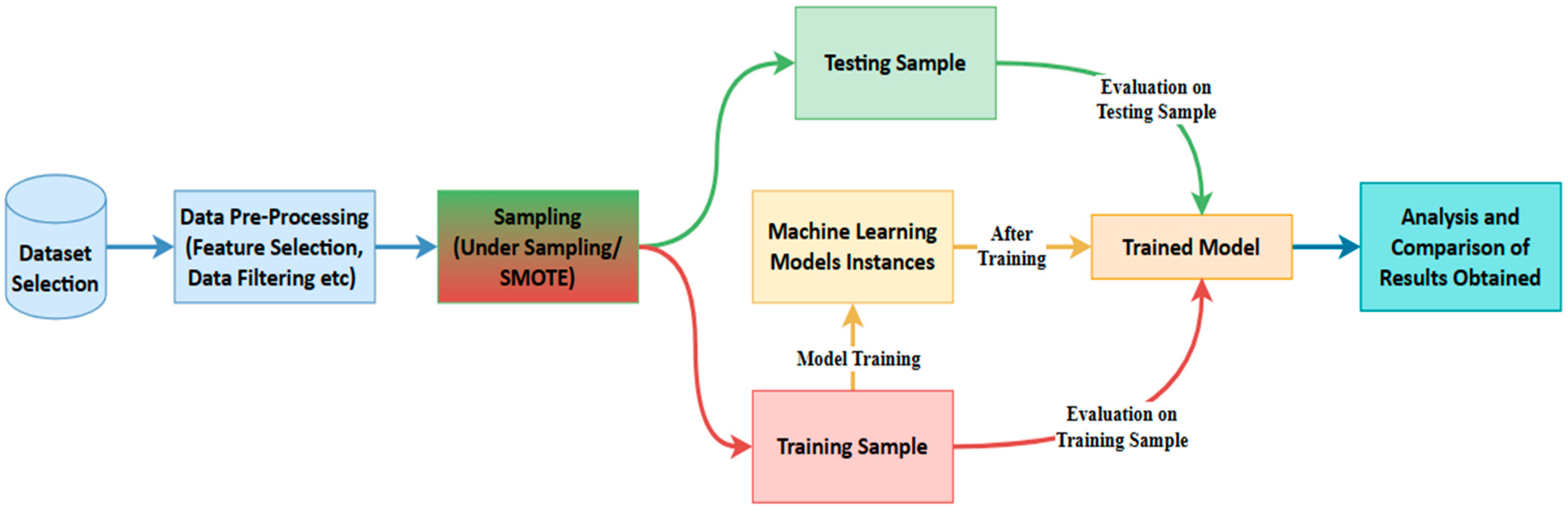
Machine learning detects fraud by leveraging historical data on both fraudulent and non-fraudulent transactions. ML algorithms excel at identifying abnormalities in transactions before they escalate into unmanageable issues. Figure 1 illustrates the flow diagram depicting how machine learning detects credit card fraud.
As shown in Figure 1, the initial step in the process involves selecting a dataset containing records of both legitimate and fraudulent transactions. Due to the presence of unordered, raw, missing, or duplicate instances in the dataset, system predictions may be prone to inaccuracies, requiring data pre-processing. To address data imbalance, the sampling of imbalanced datasets is performed. Subsequently, the organised and sampled data are divided into training and testing samples, where the chosen machine learning models are trained using the training sample, and both samples are employed to observe the behaviour of the trained models. Following the acquisition of results for selected evaluation parameters such as accuracy, precision, recall, confusion matrix, and AU-ROC values, performance is analysed and compared. The methodology employed in this paper adopts an experimental design, aiming to create and execute a practical experiment for credit card fraud detection.
3.1. Dataset
For our model training and testing, the Credit Card Fraud Detection dataset [33] was utilised. The dataset contained records of transactions conducted by European credit cardholders over two days. In the dataset, there were 492 instances of fraud out of a total of 284,807 transactions during the specified time frame. Notably, the dataset exhibited significant skewness, with the positive class (frauds) representing only 0.172% of all transactions. Each transaction in the dataset was associated with 28 additional features labelled as V1–V28. Due to confidentiality concerns, these features were transformed using Principal Component Analysis (PCA). It is important to note that the ‘Time’ and ‘Amount’ features were exceptions to this transformation; PCA did not alter them. The ‘Time’ feature represents the elapsed time in seconds between each transaction and the first transaction in the dataset. On the other hand, the ‘Amount’ feature corresponds to the transaction amount [29].
As previously stated, the dataset utilised in this paper exhibited a pronounced skewness attributable to the few fraud entries. The efficacy of training and testing the model was significantly compromised when conducted on such imbalanced datasets [34]. To address this challenge, two methodologies were employed: under-sampling and Synthetic Minority Over-sampling Technique (SMOTE). In the under-sampling approach, 492 entries were randomly selected from the 284,315 legitimate entries to achieve a balanced distribution of 50% for each class (legitimate and fraud). Conversely, the SMOTE technique involved oversampling 492 instances to augment the fraud class to match the volume of legitimate entries, resulting in an equitable representation of each class.
The ethical dimensions inherent in the dataset of this project encompass issues of data ownership, consent, and privacy. The ULB Machine Learning Group oversees the dataset in collaboration with Worldline. This collaborative initiative underscores a collective research endeavour that seamlessly integrates big data mining and fraud detection [33]. Nonetheless, this scientific undertaking harbours a discreet decision to transform dataset attributes into numerical entities through the application of Principal Component Analysis. This pivotal ethical transition underscores dedication to safeguarding the distinct intricacies of individual transactions while navigating the forefront of data science. It prompts contemplation regarding the delicate equilibrium between the pursuit of scientific knowledge and the ethical obligation associated with harnessing the formidable power inherent in datasets teeming with financial activities [35].
3.2. The Proposed Model
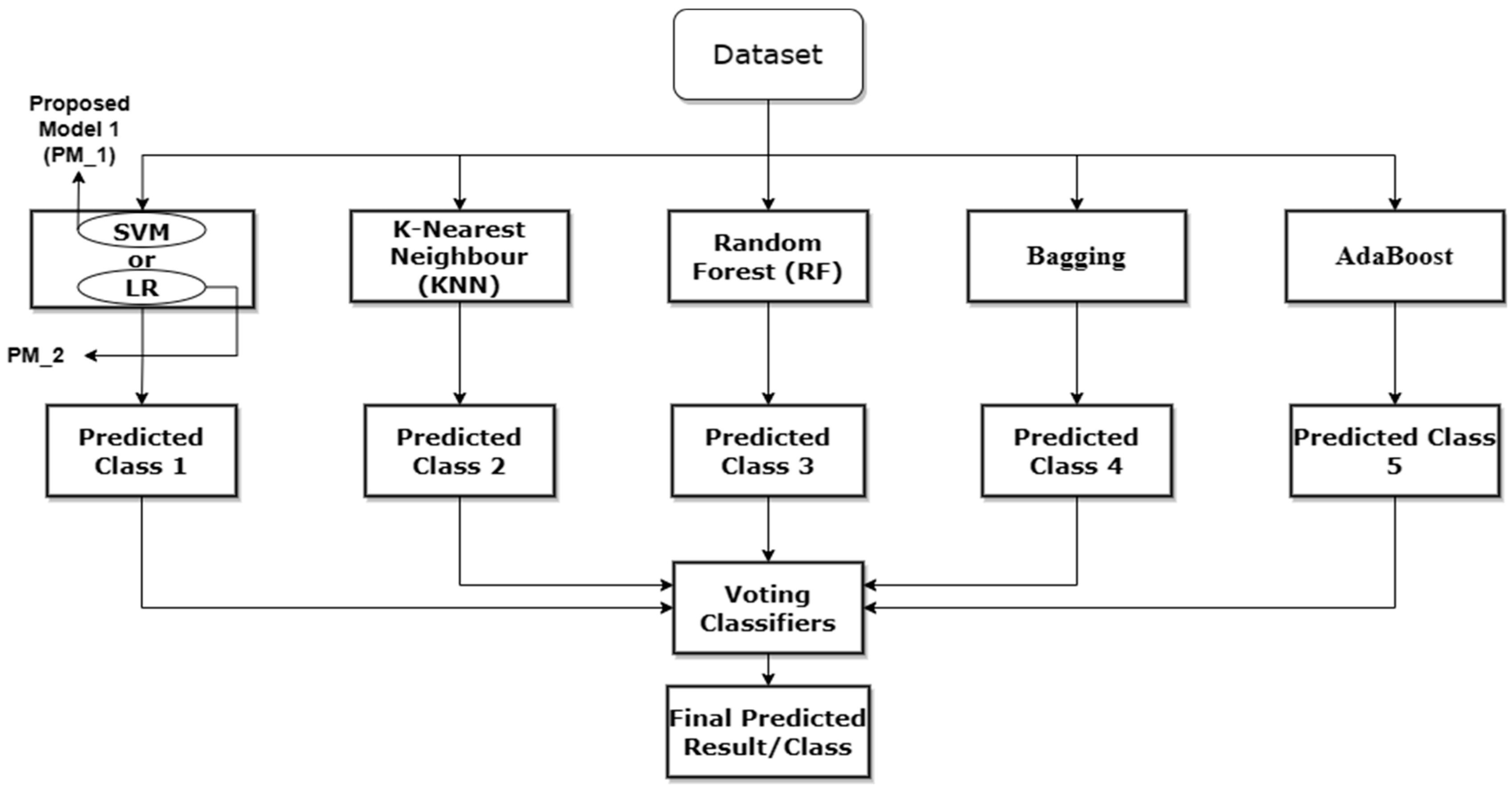
The proposed model for this paper is displayed in Figure 2. The experimental approach, contents, and architecture were designed using insights and findings from the existing literature to ensure that the experiment is relevant and appropriate for investigating the real-world occurrence of credit card fraud.
The experimental design of our proposed model was selected to test and assess fraud detection strategies in a controlled environment. This approach allowed for variable manipulation and cause-and-effect analysis, which is vital for assessing ensemble credit card fraud detection solutions. The work used a practical experiment to reconcile theoretical concepts and real-world applications, providing insights for constructing a strong and efficient fraud prevention system.
The ensemble machine learning approach used in this paper combines various classifiers, each chosen for its distinct capabilities. SVM excels in determining appropriate hyperplanes for class separation [18], whereas Logistic Regression (LR) models event probability. Random Forest (RF) builds robust decision trees [21], while K-Nearest Neighbors (KNN) performs classification based on the majority class among its nearest neighbours [19]. Bagging uses KNN as its basic classifier to enrich the ensemble further. Boosting uses RF as its base [36]. An important contribution is the Voting Classifier, which combines the various predictions from these classifiers. All of these choices were thoughtfully determined based on their demonstrated performance in earlier research, which was thoroughly detailed in the literature study. This extensive ensemble of classifiers is a deliberate tactic aiming to improve the prediction power of the proposed model.
The ensemble machine learning classifiers were adopted in this paper due to their superior performance when dealing with datasets containing limited labelled data, as exemplified in this paper. Credit card fraud datasets often exhibit imbalances, where fraudulent transactions constitute a small fraction of the overall data [6]. Ensemble methods excel in addressing class imbalances, demonstrating robust performance in detecting minority classes. Moreover, ensemble models contribute to interpretability and transparency in decision-making, crucial attributes in financial domains where understanding the model’s rationale is essential. They facilitate the aggregation of diverse weak learners, thereby enhancing the overall predictive capabilities of the model. Additionally, ensembles prove to be computationally less intensive compared to deep learning architectures, rendering them more suitable for scenarios with constrained computational resources [4].
The process of developing the suggested ensemble model involved a careful examination of different base classifiers and weighting schemes. The ensemble combined Support Vector Machines (SVM), K-Nearest Neighbors (KNN), Random Forest (RF), Bagging, Adaboost, and a voting classifier. The SVM model was thoroughly evaluated across multiple configurations, which involved testing different regularisation values ranging from 1.0 to 10 and various kernels such as linear, poly, and rbf. Interestingly, the highest level of efficiency was achieved with the default setup parameters during both the training and testing phases. Similarly, KNN and RF were examined using various values for n-neighbors (ranging from 2.0 to 10) and n-estimators (ranging from 10 to 100). The analysis showed that the default parameters produced the best outcomes. Since Bagging and Boosting are ensemble algorithms, KNN and RF were used as base classifiers with their default settings. Significantly, these varied arrangements were assessed on a dataset that had a lower number of samples, resulting in faster training and evaluation processes compared to the SMOTE dataset.
3.3. Hardware and Platforms
The experimental setup was supported by hardware and cloud resources. The local computer was outfitted with an Intel(R) Core (TM) i5-2520M CPU running at 2.50 GHz and 12 GB of RAM, ensuring efficient processing and memory for the tasks at hand. The storage capacity of the local machine was sufficient for hosting the dataset and project files, with an extra 900 GB of cloud-based storage readily available when needed. The work primarily occurred in a cloud environment equipped with 12.68 GB of RAM and approximately 107.72 GB of disk space. These cloud-based resources significantly enhanced the computational power necessary for tasks such as data processing, model creation, and training.
The selection of platforms and tools for our proposed model was guided by considerations such as usability, compatibility with chosen machine-learning techniques, and the availability of pre-trained models. Notably, the well-established machine learning framework, sci-kit-learn, was employed. In terms of data pre-processing, feature extraction, and exploratory data analysis, the proposed model leveraged the efficiency of pandas, NumPy, and Matplotlib. Together, these libraries provided robust capabilities for data manipulation and analysis, streamlining tasks related to data processing and exploration. For model creation and training, we utilised Google Colab, a cloud-based platform recognised for its flexibility and resource efficiency, particularly compared to conventional platforms like Jupyter Notebook. The cloud-based architecture of Google Colab facilitated convenient access to computational resources. A comprehensive set of metrics was employed to evaluate machine learning models, encompassing accuracy, precision, recall, F1-score, confusion metrics, ROC Curve, and AU-ROC Score. Visualisation packages such as Matplotlib and Seaborn were employed to enhance data understanding and assess model performance. These libraries aided in constructing graphical representations that provided insights into data trends, model performance, and the significance of dataset aspects.
3.4. Model Design
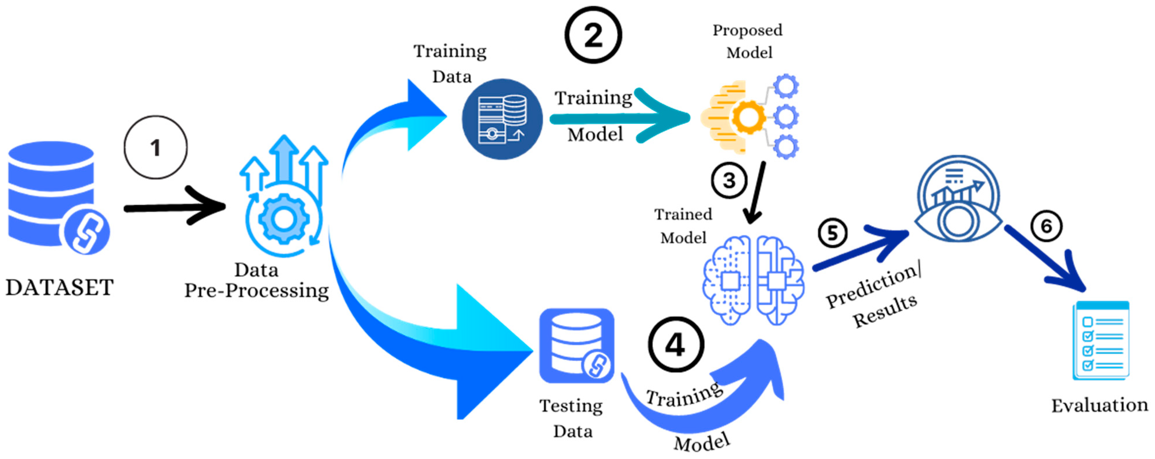
Figure 3 displays the architecture of the implementation process, encompassing dataset pre-processing and the division of the dataset into training and testing data. The training dataset is subsequently input into the chosen models for both the training and testing phases. Following this, the evaluation and results are conducted on the trained model to assess its performance.
Algorithm 1 presents the algorithm of the proposed model. The algorithm follows a systematic approach, starting with data loading, preprocessing, and sampling. The numbers in Figure 3 explains the sequence of each phase in the whole process. It then iterates over different machine learning model types, trains each model, and evaluates their performance using testing data. Finally, the results, including confusion matrices, are displayed for analysis.
| Algorithm 1 Credit Card Fraud Detection Using Ensemble Machine Learning Models | |
| Input: | Credit_Card_Fraud_Dataset |
| Output: | Trained_Machine_Learning_Models |
| 1. | dataset ß Load_CreditCard_Fraud_Dataset() |
| 2. | processed_data ß PreprocessedData(dataset) |
| 3. | labels ß (processed_data) |
| 4. | under_sampled_data ß (labels) |
| 5. | smote_data ß (labels) |
| 6. | for model_type in [‘SVM’, ‘RF’, ‘Bagging’, ‘Boosting’, ‘LR’, ‘P_M_1’, ‘P_M_2’]: |
| 7. | training_data, testing_data ß TrainTestSplit(under_sampled_data) |
| 8. | if model_type == model: |
| 9. | model ß model_type |
| 10. | elif model_type == ‘Proposed_model’ |
| 11. | models.append(mode_type) |
| 12. | for model_type, model in models: |
| 13. | testing_data_features ß tresting_data.drop(‘Class’) |
| 14. | testing_data_labels ß testing_data[‘Class’] |
| 15. | confusion_matrix ß Evaluate_model(model, testing_data_features, testing_data_labels) |
| 16. | endif |
| 17. | end for |
| 18. | return display_results ß (confusion_matrix, model_type) |
3.4.1. Data Pre-Processing
After selecting the dataset, the first step is to pre-process the data to make it suitable for model training and testing. In this step, the data were processed in the following ways.
- Finding and filling/removing any null values.
- Standardising the ‘Amount’ column to make it easy for analysis.
- Removing the ‘Time’ Column from the dataset as it was not contributing much during training and evaluation.
- Checking and removing duplicate entries in the dataset.
The dataset used in the process was devoid of any missing or null values. It is important to mention that intentional actions to reduce the influence of outliers were not included. The conclusion was based on the understanding that the selected machine-learning model is naturally resistant to outliers. Moreover, incorporating outliers into the dataset was considered advantageous since it brings the model into closer alignment with the complexities of real-world situations. This study sought to improve the model’s capacity to handle the dynamic and different nature of credit card transactions by not using explicit outlier-handling strategies. This approach made the model more adaptable and applicable to real-world scenarios.
The reason for standardising the ‘Amount’ column instead of normalising it is that, as mentioned in the description of the dataset, all features were the result of Principal Component Analysis (PCA) except ‘Time’ and ‘Amount’, and the ‘Amount’ scale differed significantly from all other features (V1–V28). Hence, the ‘Amount’ feature was standardised.
The feature engineering component of this credit card fraud detection research was complicated by the intrinsic limitations imposed by the dataset, which did not provide information about its features [33]. Therefore, the use of feature selection techniques was not possible because it would have required clear visibility of feature information. To avoid any potential confusion caused by algorithmic feature selection, a deliberate choice was made to abstain from this process. Furthermore, the ‘Time’ column was excluded from consideration during manual analysis because it did not contribute any meaningful information. It only reflected a sequential count of entries without any temporal significance. Although the lack of feature selection techniques may result in longer training and testing durations, this strategy was considered the best choice to guarantee the retention of all potentially relevant features without relying on feature-specific knowledge.
3.4.2. Data Sampling
Following pre-processing, the subsequent step in the process involved addressing the data imbalance issue through data sampling. After pre-processing, the dataset comprised 275,190 legitimate entries and 473 fraud-labelled entries, indicating a significant skewness for model training. This paper employed two sampling techniques: under-sampling and SMOTE. The sampling process involved two steps, outlined as follows:
- Separate data entries based on labels (Legit/Fraud in this case)
- Apply the required sampling technique to specific data
- Concatenate all data to have all data in a single dataset
Under-Sampling
In sampling, a random sample was picked from the major class, which were legit transactions (labelled as 0) in this case. The number of random samples was determined according to the ratio required concerning the minority class. In this paper, for better model training, the entries for both classes were made equal by choosing a random sample equal to minority class entries and concatenating the data from both classes to have one dataset.
SMOTE (Synthetic Minority Over-Sampling Technique)
SMOTE is a statistical method for extending the number of minority class instances in a balanced manner in a dataset. The component created new instances from existing minority cases that were provided as input [37]. So, for SMOTE, the fraud class (labelled as 1) was oversampled, equal to the legit class to have identical entries for each class to train models optimally. And like under-sampling, both classes were merged to have one dataset.
3.4.3. Model Training
After the sampling process, the subsequent step involved splitting the data into training and testing samples. The training samples were utilised for model training and result assessment, while the testing samples were employed to evaluate how the model performs on unseen data. Before the data split, the ‘Class’ column, containing the label of each entry, was separated. The dataset was then divided into training (80% of the dataset) and testing samples (20% of the dataset). Following this, the training sample was employed for model training. Once the models were trained, evaluations were conducted on both the training and testing samples, with the results discussed in the next section.
After carefully dividing the dataset into training and testing samples, the model training phase focused on identifying patterns and relationships in the data. The chosen machine learning algorithms utilised the training samples to undertake a detailed process of learning and adjusting to the complexities of credit card transaction characteristics. The model-refining method involved iteratively modifying the intrinsic parameters of the algorithms to improve predicted accuracy. It is crucial to emphasise that this step goes beyond simple algorithmic integration; it involves a dynamic interaction between the algorithms and the subtle details of the dataset. This mutually beneficial interaction not only enabled the extraction of complicated patterns but also guaranteed the model’s ability to withstand real-world difficulties. Afterward, the trained models were subjected to a thorough evaluation of both the training and previously unused testing data, which provided a reliable assessment of their ability to generalize model outputs. The results of this phase, explained in the next part, reveal the effectiveness and flexibility of the developed models in successfully traversing the complex field of credit card fraud detection.
4. Results and Discussion
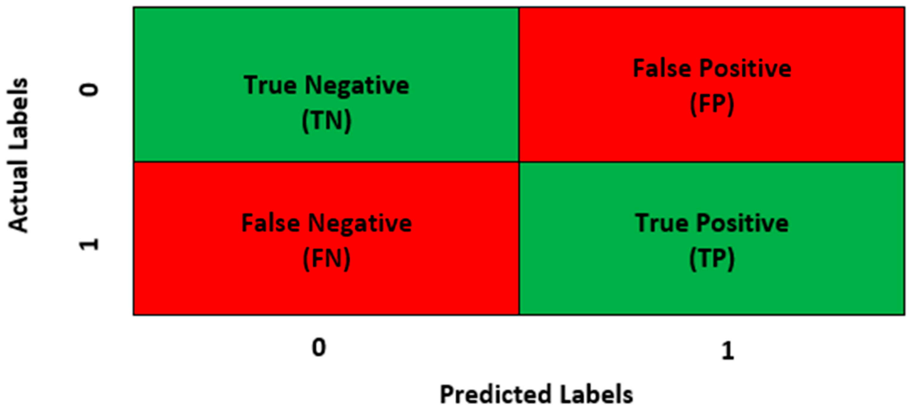
This section delves into a comprehensive discussion and analysis of the performance parameters acquired during the evaluation. It includes detailed insights into how each model performed in the context of credit card fraud detection. Prior to this discussion, the following details about the performance parameters used in this research are provided. All parameters were calculated using the True Positive (TP), True Negative (TN), False Positive (FP), and False Negative (FN) values of each model, with the confusion matrix (CM) encapsulating these values. Figure 4 visually presents a representation of the confusion matrix utilised for the proposed model, enhancing clarity and understanding.
Accuracy (ACC) is the ratio of all correct predictions (TP + TN) to the total number of predictions or entries in the sample (TP + TN + FN + FP) [38]. Equations (1)–(4) show the mathematical representation of how the Accuracy, Precision, Recall, and Fi-score of a model are calculated.
Precision is the ratio of TP to all positive predictions (TP + FP) made by a model. In other words, it is the accuracy of the positive predictions made by the model.
Recall is a metric used to measure the ability of the machine learning model to identify all relevant instances of the positive class [39]. It is the ratio of correctly predicted positive observations to the total actual positive observations.
F1-score is a metric used to combine the results of precision and recall into a single value. The formula of the F1-score is as follows.
4.1. Performance Evaluation
The performance evaluation for both Under-sampling and SMOTE samples for each model are divulged in the sections below.
4.1.1. Under-Sampling Results
The results of the confusion matrix obtained during the evaluation of each model for under-sampling are presented in Table 2.
Based on the provided results, both RF and boosting models exhibited 0 false positive and false negative values, indicating accurate predictions for both classes. The second proposed model predicted all negative class values accurately but misclassified 20 positive class values. The proposed model with SVM (P_M_1) ranked third, with 24 false predictions for positive class values. However, relying solely on these results, derived from the data sample used for model training, is insufficient, as the models are already familiar with these data points. To assess how the models respond to unseen data, the evaluation was conducted on a testing sample of under-sampled data. Additionally, examining the results of the prediction sample helps ensure that machine learning models are optimally trained, avoiding underfitting or overfitting. Table 3 displays the values of the confusion matrix for all models obtained from the testing Sample.
The comparison of results between Table 2 and Table 3 indicates that the models are optimally fitted, as the results obtained from both samples are consistent (further clarified in the discussion of other parameters). According to these findings, the second proposed model with LR (P_M_2) and bagging outperformed all other models, with ten values predicted falsely (8 FP, 2 FN). As mentioned earlier, accuracy is the ratio of all correct predictions to the total number of predictions or entries in the sample [38]. Table 4 shows the accuracy values of all models on the training sample and testing sample.
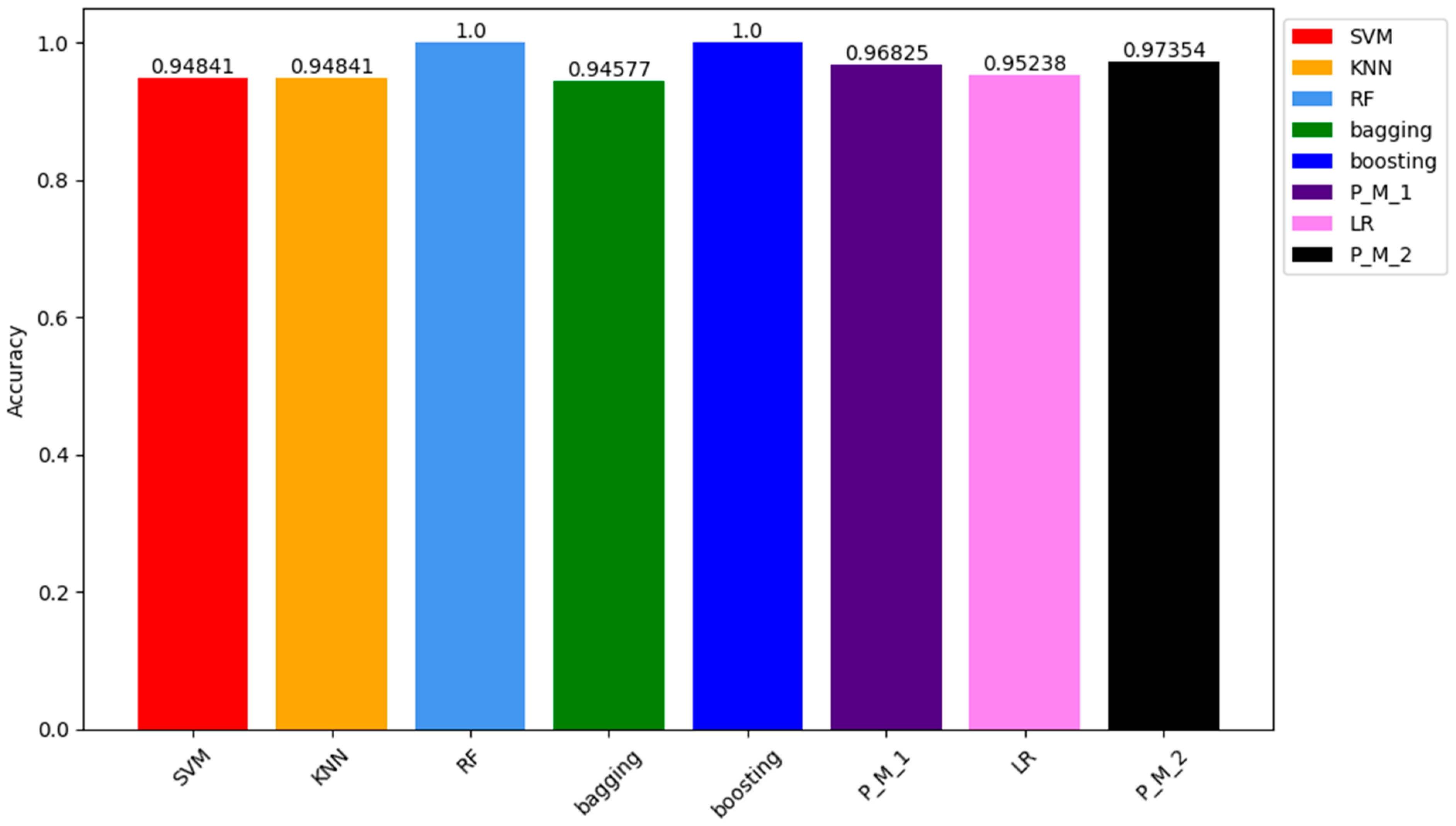
Similar to the results of the confusion matrix for training samples, the ACC of RF and Boosting models is 100%. The ACC of other models, including P_M_1, P_M_2, LR, SVM, KNN, and bagging, are 97.35%, 96.82%, 95.23%, 94.81%, 94.81%, and 94.57%, respectively. Figure 5 visually represents these values through a bar chart. Each colour in the chart corresponds to a model, with details about the colour and corresponding model specified in the legend box located at the top right corner.
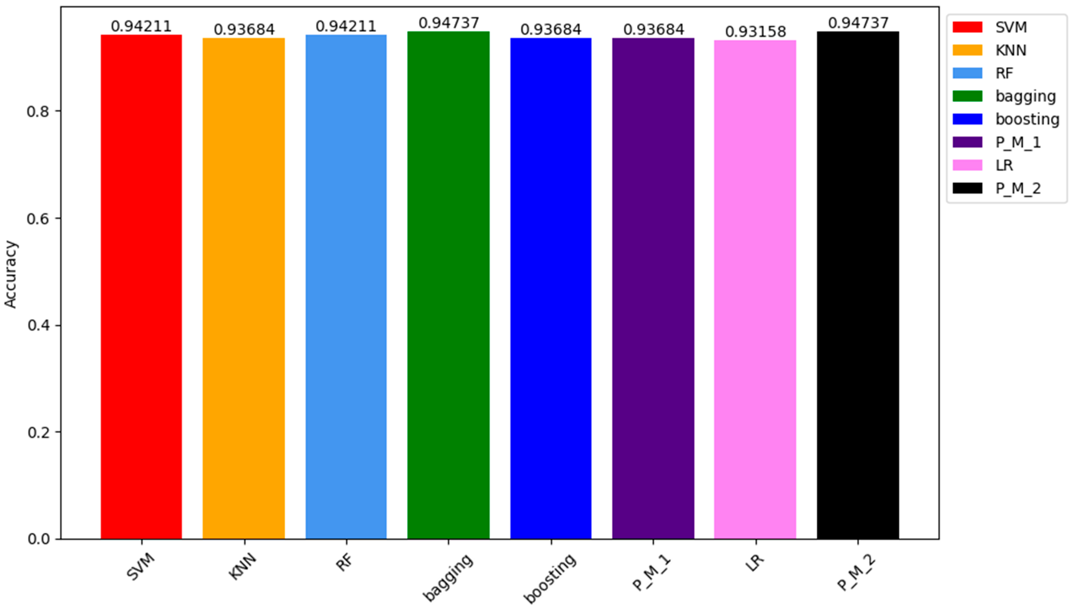
In the results obtained from the testing sample, the ACC of P_M_2 and the bagging classifier were the highest among all models, reaching 94.73%. Following closely were the ACC values of SVM and RF classifiers, both at 94.21%. The ACC of KNN, Boosting, P_M_1, and LR classifiers were 93.68%, 93.68%, 93.68%, and 93.0%, respectively. The graphical representation of these results can be seen in Figure 6, which depicts how models respond to the unseen data.
The precision, recall, and F1-score of a machine learning model explain how well a classifier performs, rather than just relying on overall accuracy [39]. The results of these parameters obtained on the training sample are listed in Table 5.
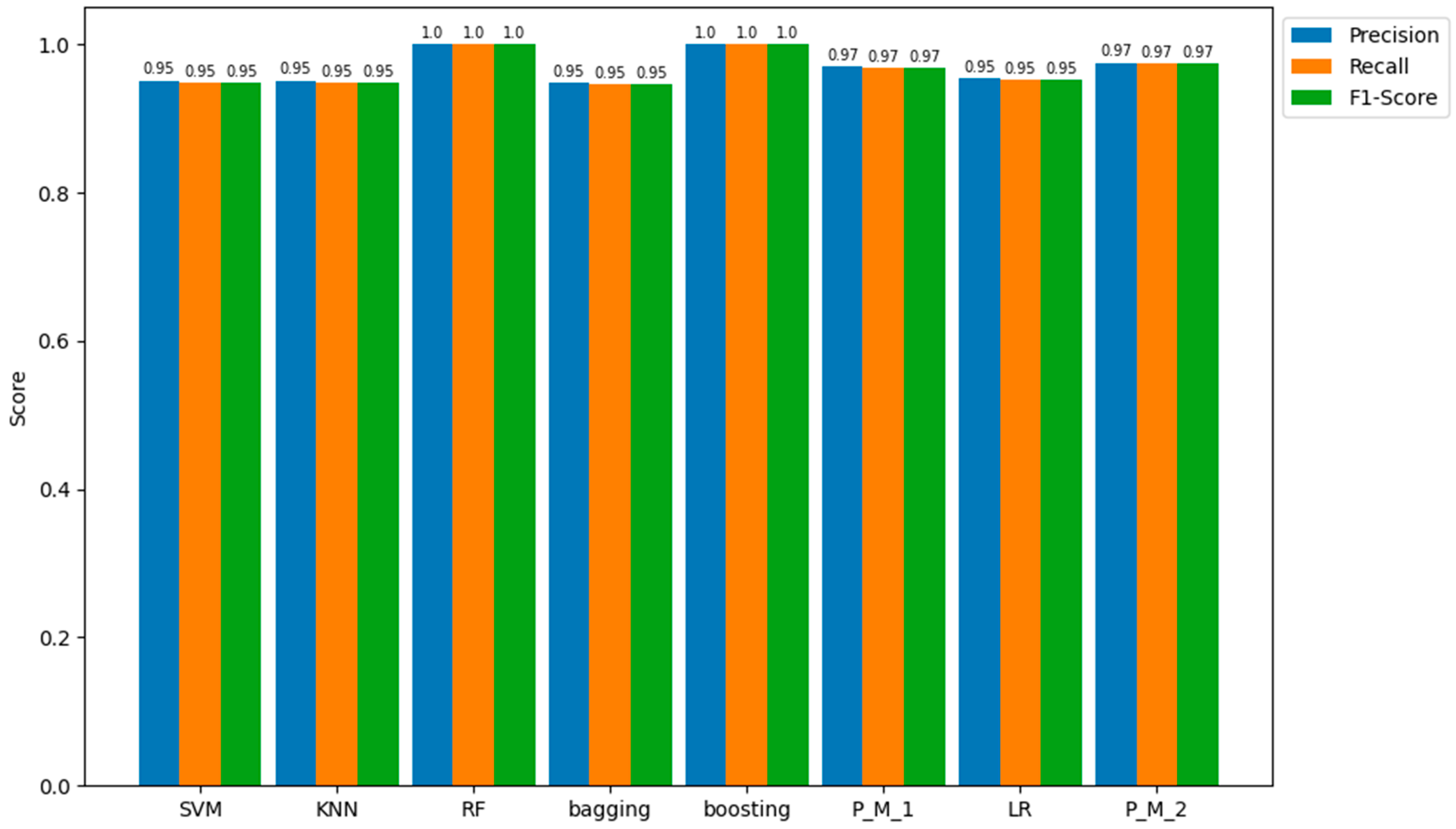
In line with the confusion matrix and ACC values, the RF and boosting classifiers demonstrated 100% precision (accuracy of positive prediction) and 100% recall (ability to identify the positive class correctly). Next to the best-performing classifiers are P_M_2 and P_M_1, both achieving an accuracy of 97%. Subsequently, SVM, KNN, bagging, and LR each attained results of 95%. The representation of these parameters is visually presented in Figure 7.
Likewise, Table 6 presents the results for precision, recall, and F1-score for all models when applied to unseen samples of the under-sampled data.
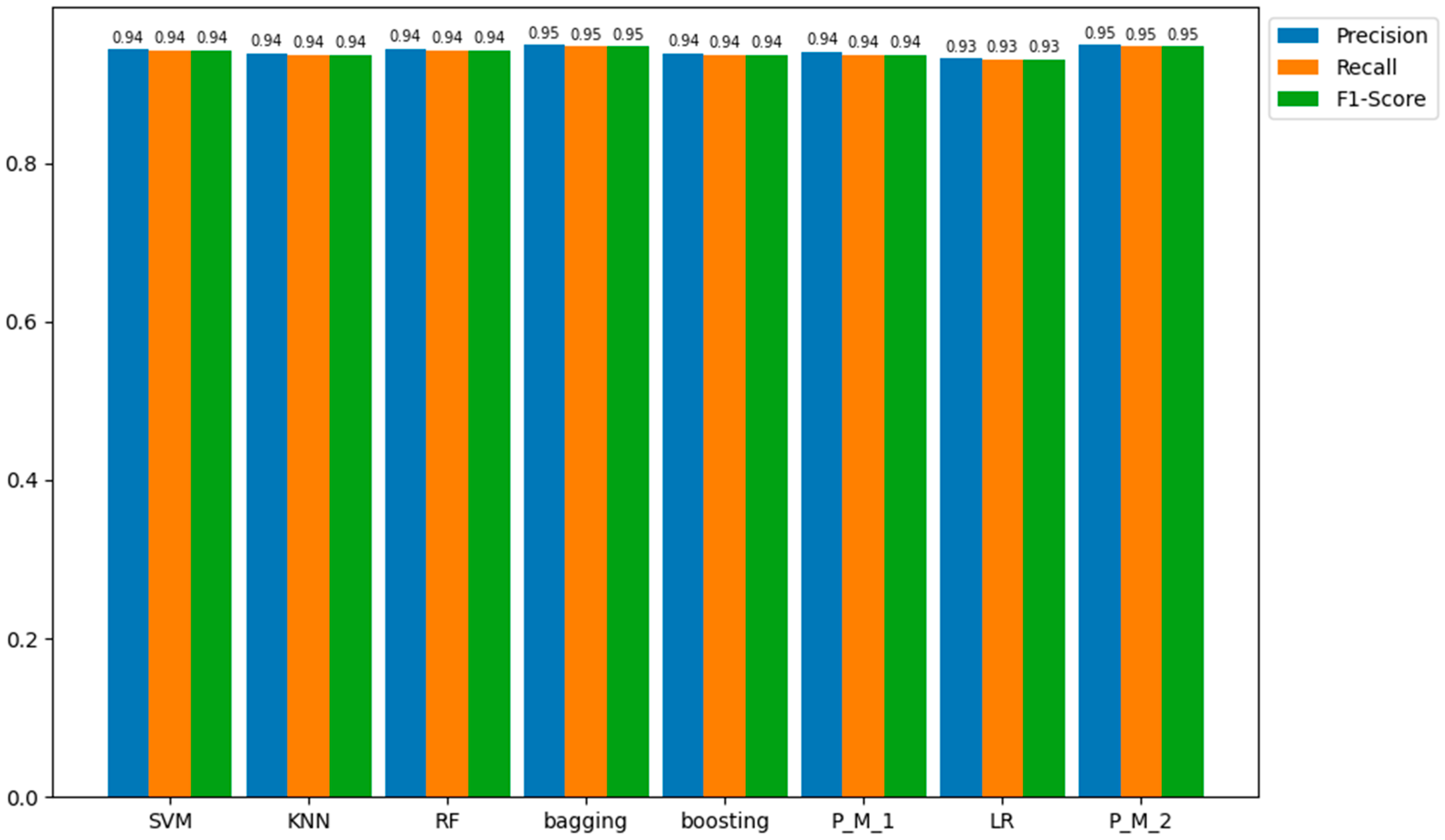
Regarding the outcomes from the testing samples, the proposed model with LR (P_M_2) emerges as the most proficient among all models in predicting the positive class (fraud), achieving precision, recall, and an F1-score of 95%. In comparison, the other models—bagging, SVM, KNN, RF, boosting, P_M_1, and LR—display precision, recall, and F1-score values of 95.0%, 94.0%, 94.0%, 94.0%, 94.0%, 94.0%, 94.0%, and 94.0%, respectively. These quantitative values are represented in Figure 8 for a more detailed understanding of these results.
The ROC curve presented in Figure 9 illustrates the trade-off between the true positive rate (sensitivity or recall) and the false positive rate as the classifier’s decision threshold varies. The ROC curve is generated by plotting the true positive rate (TPR) on the y-axis against the false positive rate (FPR) on the x-axis at different classification thresholds. Figure 9 displays the ROC curve for all models, with the corresponding AUC-ROC values of each model indicated in the bottom right corner of the image.
The ROC curves highlight distinct trade-offs between sensitivity and specificity across our models. AUC-ROC values provide a concise overview of the overall ability of the model to distinguish between positive and negative examples, with larger values indicating superior performance. Notably, the Support Vector Machine (SVM) model exhibited the highest Area Under the Receiver Operating Characteristic Curve (AUC-ROC) value at 0.9846, signifying robust discriminatory capabilities. Furthermore, the Logistic Regression (LR) K Nearest Neighbor (KNN) and our proposed models (P_M_1 and P_M_2) emerge as strong contenders, with AUC-ROC values surpassing 0.979.
4.1.2. SMOTE Results
All the training and testing results presented in this section were obtained using the SMOTE sampled dataset. Similar to the previous section, we begin by discussing the results of the confusion matrix for all models, as other parameters are derived from TP, FP, TN, and FN values, and the confusion matrix encompasses all of these values. Table 7 shows the confusion matrix for all models obtained for the oversampled dataset training sample. These confusion matrices represent the results of predictions for 440,304 entries or values present in the training sample.
The results indicate that, similar to the under-sampled dataset, RF and Boosting classifiers emerged as the top-performing models, making no false predictions on the trained sample. The proposed model followed closely, exhibiting 70 false negative values and no false positive values. Subsequently, KNN and Bagging showed 284 and 288 false negative values, respectively, with no false positives. LR ranked last, displaying the highest false negative and false positive values. Table 8 shows the prediction of models on the unseen sample (Testing sample).
According to the results obtained from the testing sample of 110,076 entries, which were unknown entries to machine learning models, RF and boosting showed the same results with 10 FN values and no FP, which were the best results compared to other models. The proposed model was second with 45 FN and 0 FP prediction, followed by KNN and bagging classifiers, with 91 and 97 FN and 0 FP predictions, respectively. LR showed the highest FN and FP results again. For a detailed evaluation of these models, other performance parameters results are discussed in the next sections. To see how accurately all models predict the training sample and testing sample, Table 9 summarises the accuracy prediction results of all the models.
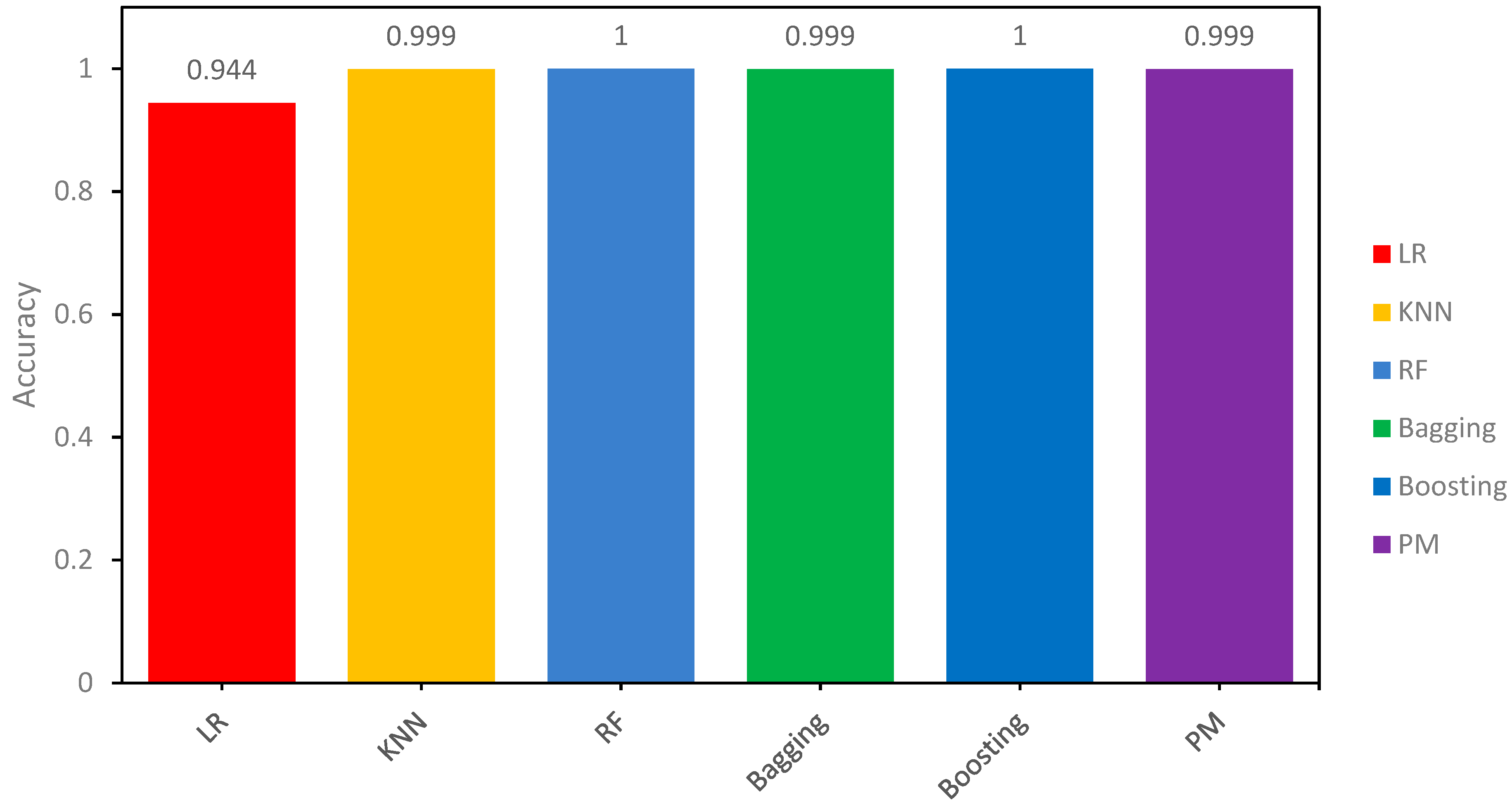
Concerning the training samples PM (Proposed Model) results, Adaboost and RF showed about 100% accuracy on the seen or training sample while KNN and Bagging classifiers had 99.93% accuracy and LR was ranked last with the lowest accuracy at 94.44%. Figure 10 shows the comparison results of all the models.
The accuracy results of all models on the testing sample are also shown in Table 9 to demonstrate how the proposed models respond to new data. Results on the unseen data show that the proposed models (PM) alongside Adaboost and Random Forest (RF) classifiers demonstrate significantly high accuracy, with all three converging at roughly 100% on the testing samples. This outcome highlights the effectiveness of these models in comprehending the underlying patterns present in the training data, resulting in predictions that nearly correspond to the accurate labels. Equally noteworthy, the K-Nearest Neighbors (KNN) and Bagging classifiers have a remarkable accuracy rate of 99.93%. These results are also presented visually in Figure 11.
This visual representation of the outcomes underscores the adeptness of models in extracting valuable insights from the provided training data. In contrast, Logistic Regression (LR) demonstrates a lower accuracy rate of 94.44%, indicating a relatively higher rate of misclassification compared to other models. Given the consistent presence of these patterns throughout the training sample, it reaffirms the stability and generalizability of our proposed model.
Table 10 consolidates the results of our analysis, specifically focusing on the evaluation metrics of precision, recall, and F1-score. This comprehensive depiction demonstrates the models’ performance in accurately predicting the positive class within the training sample, elucidating their proficiency in correctly assessing positive class predictions (recall) and the equilibrium between these two metrics as reflected in the F1-score.
In a parallel evaluation of the results of the confusion matrix, we observe a consistent trend in the precision, recall, and accuracy metrics across our models compared to both the training and testing samples. Particularly, the majority of models have precision, recall, and accuracy scores around 100 percent, demonstrating their proficiency in correctly classifying positive instances, as shown in Figure 12.
Based on the results and visual representations, it is evident that these models adeptly capture relevant data, leading to precise predictions and minimal false negatives. Despite this outstanding performance, the Logistic Regression (LR) model stands out with slightly lower yet commendable precision, recall, and accuracy scores of 95.0%. This distinction highlights the sensitivity of the LR classifier to specific data complexities while affirming the overall robustness of the results obtained by other classifiers. As mentioned earlier, the results for precision, recall, and F1-score obtained for both training and testing samples are consistent, as verified by the data presented in Table 11 and Figure 13.
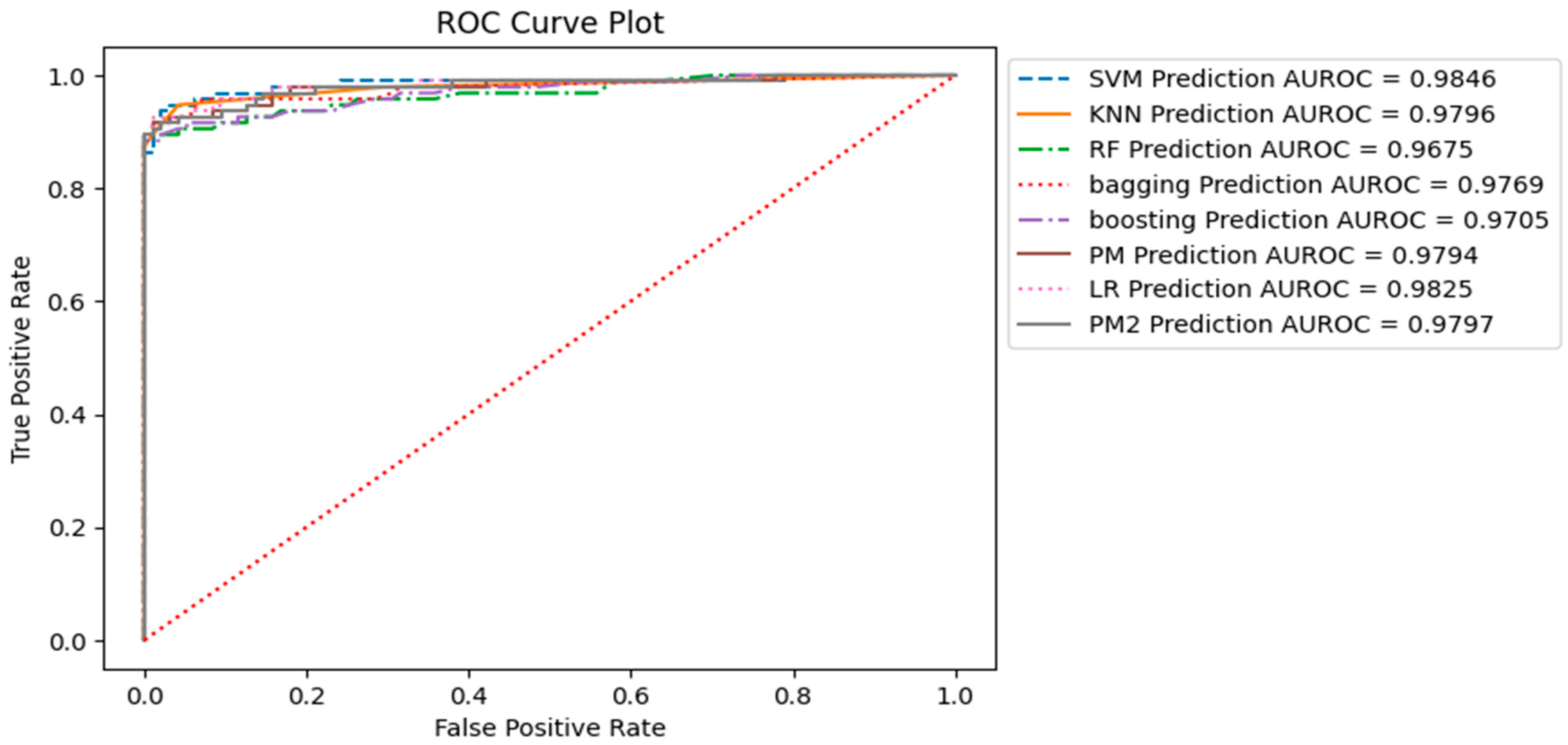
All ROC curves obtained from the SMOTE-sampled dataset, including Support Vector Machine (SVM), K-Nearest Neighbors (KNN), Random Forest (RF), Bagging, AdaBoost, and the proposed model (PM), exhibit exceptional performance, as indicated by the steep ascent towards the upper-left corner of the graph. This demonstrates that these models achieve high sensitivity while maintaining low false positive rates, highlighting their ability to classify positive instances while minimising misclassifications of negative instances accurately. Figure 14 shows the results of the ROC curve of all models, with the AUC-ROC values of all models shown in the bottom right corner.
The AUC-ROC values offer a quantitative assessment of the capability of the models. The AUC-ROC values, which range from 0.988 to 0.999, highlight the exceptional performance exhibited by all the models. A higher AUC-ROC value indicates a stronger discriminatory ability of the model to distinguish between positive and negative events. In this comparative analysis, the AUC-ROC values continually converge towards or even attain a value of 1, validating the excellent predictive capacities exhibited by the models. The high AUC-ROC values observed in these models suggest a constant ability to predict genuine positives while effectively minimising false positives accurately. The combined utilisation of ROC curve analysis and the notable AUC-ROC values demonstrates the effectiveness of the models under consideration in accurately distinguishing between positive and negative occurrences.
4.2. Computational Efficiency
Computational efficiency in Machine Learning pertains to the time an algorithm requires for training and evaluation, as well as the utilisation of system resources such as RAM and storage during these processes. In this paper, the python-auto time and memory-profiler extensions were employed to measure the training and evaluation durations and the RAM usage, respectively. RAM usage was documented both before and after each training and testing phase, with the results summarised in Table 12.
The collected data revealed variations in training and testing times among the different algorithms. Notably, some algorithms, such as LR, SVM, and KNN, exhibited longer training times but shorter testing times, while others demonstrated the opposite trend. RAM usage values in the table are presented in units of Mebibyte (MiB), where 1 MiB is equivalent to 1.04858 MB. It is crucial to emphasise that RAM usage values were recorded both before and after each training and testing phase.
Furthermore, Figure 15 illustrates random RAM usage values noted during the training and testing phases. These fluctuations indicate that RAM usage ranged between 2.3 to 4.0 GB during these phases. Specifically, in the case of SMOTE, where the training dataset comprised 440,304 entries, the highest time recorded for evaluating results on these entries was 11,681 s. Consequently, the system identified approximately 38 entries per second as either legitimate or fraudulent during the utilisation of these computational resources.
The RAM usage values presented in Table 12 were documented in Mebibyte (MiB), with the conversion factor of 1 MiB equaling 1.04858 MB. Additionally, the computational resource usage values were carefully recorded just before and after each training and testing phase. In tandem with these measurements, random values of RAM usage were also observed throughout the training and testing phases. Analysis of these random values indicates that the RAM usage fluctuated between 2.3 to 4.0 GB during both the training and testing phases. A visual representation of the time taken by each algorithm in the training and testing phases is shown in Figure 15 and Figure 16. These graphical representations provide insights into the efficiency and performance of each algorithm throughout the different stages of the machine-learning process.
As depicted in Figure 15 and Figure 16, certain algorithms, such as LR, KNN, and Adaboost, exhibited longer training times and shorter testing times. Conversely, other algorithms, including Bagging and PM, needed less training time but had longer testing times. In the case of SMOTE, where the training dataset comprised 440,304 entries, the highest time recorded for evaluating the results on these entries was 11,681 s. Consequently, utilising these computational resources, the system demonstrated the capability to identify approximately 38 entries per second as either legitimate or fraudulent. These observations provide valuable insights into the performance characteristics of each algorithm during both the training and testing phases.
4.3. Comparison with Existing Models
As in the literature review of this paper, different studies have been summarised in Table 1. The models proposed in [1,40] are comparable to the models proposed in this paper. In [40], the proposed model consisted of a K-Nearest Neighbor (K-NN), Extreme Learning Machine (ELM), Random Forest (RF), Multilayer Perceptron (MLP), and Bagging classifier while the dataset used is different than that used in this research. In [1], the proposed model contained Random Forest (RF), K-Nearest Neighbors (KNN), Logistic Regression (LR), Adaboost, and Bagging, similar to P_M_2 in under-sampling and PM in SMOTE. In [1], SMOTE was used for an unbalanced dataset, which was also used for our proposed model. Table 13 and Figure 17 show the evaluation metrics adopted for the benchmarking of the proposed model.
The accuracy achieved by the present model [28] is 83.83%, which is significantly lower compared to the accuracy achieved by our proposed model. This observation implies that there may be certain constraints in the accurate classification of cases, as shown by [24]. The proposed model in [25] had a strong performance, with an accuracy percentage of 99.9455%. Although it demonstrated a high level of precision, it is crucial to consider additional measures to offer a thorough evaluation. The proposed model, PM (SMOTE), demonstrated exceptional performance with an accuracy of 99.9591%, exceeding the results achieved by both references [17,28]. This suggests that the PM (SMOTE) algorithm demonstrates a noteworthy capability in accurately classifying cases, perhaps leading to enhanced skills in fraud detection.
P_M_1 and P_M_2, two more models under consideration, exhibited comparable or somewhat inferior performance in accuracy, precision, recall, and F1-score compared to the PM (SMOTE) model. The P_M_2 is the same model as PM; the only difference is the sampling technique used for the dataset. In P_M_2, under-sampling was used, while in the PM, SMOTE was used as a sampling technique. This implies that the utilisation of under-sampling as the sampling strategy in P_M_1 and P_M_2 may have resulted in a decrease in the size of the dataset. Although the process of reducing class distribution might contribute to achieving a balanced distribution in a class, it is important to acknowledge that this approach may lead to a certain degree of information loss. Consequently, the performance of this method may be comparatively weaker than the PM (SMOTE) technique.
In summary, the assessment findings underscore the merits and limitations of different approaches. The PM (SMOTE) technique demonstrated superior performance, exhibiting the greatest levels of accuracy, precision, and F1 score. Nevertheless, it is crucial to consider the contextual factors and trade-offs that are linked to various sampling approaches. The utilisation of under-sampling, as seen in P_M_1 and P_M_2, might potentially impact the overall performance of the model. When selecting an appropriate model, it is important to consider the particular objectives and limitations associated with the work of credit card fraud detection.
4.4. Limitations and Challenges
This research found that there were substantial challenges with credit card fraud detection. The acquisition of a suitable credit card dataset proved to be a formidable task due to the sensitivity of client data. The profound social and financial consequences associated with credit card fraud detection required thoughtful consideration at every step. Selecting appropriate classifiers in a field saturated with ongoing research in credit card fraud detection presented a unique set of challenges. The evolving nature of this subject matter made the classifier selection process particularly intricate.
While Google Colab offered a convenient implementation environment, it introduced its own set of challenges. Operating on a free cloud platform demanded vigilant attention due to its sensitivity to extended durations, network outages, and even slight deviations from attentive usage. Managing these intricacies became crucial to avoid accidental disconnections and process restarts. From the initial hurdles of dataset gathering to the complexities of classifier selection and platform nuances, these challenges underscore the intricate nature of the research landscape, contributing to a nuanced understanding of this study’s limitations.
5. Conclusions and Future Work
This paper presented an in-depth literature review that underscored the significance of the credit card fraud epidemic. The surge in identity theft, particularly through credit card fraud, has inflicted financial losses and emotional distress on countless victims. Statistics from organisations like the Federal Trade Commission (FTC) depict a disconcerting portrayal of the ever-evolving fraud landscape. To counter these challenges, we delved into various fraud detection techniques, exploring Statistical Analysis, Machine Learning, and Deep Learning Techniques for discerning suspicious patterns in transaction data.
For classification tasks, an array of machine learning models, spanning from K-Nearest Neighbors (KNN) to Support Vector Machines (SVM), Decision Trees (DT), Random Forest (RF), Bagging, and Boosting, emerged as potent instruments. In this paper, we meticulously evaluated the effectiveness of these models on a real-world dataset of European credit card transactions. These endeavours culminated in the proposition of an ensemble model that integrates SVM, KNN, RF, Bagging, and Boosting classifiers within a voting framework. This ensemble not only showcased robust performance but also underscored the efficacy of combining multiple classifiers to enhance fraud detection accuracy. During the evaluation process, the models underwent rigorous testing, and their performance was scrutinised using diverse metrics, including precision, recall, F1-score, ROC, and accuracy.
The outcomes affirmed the effectiveness of our ensemble model in mitigating false positives and false negatives, two pivotal challenges in credit card fraud detection. However, this research also provides future research opportunities. Striking a balance between accuracy and computational efficiency emerged as a crucial consideration. As demonstrated in the computational efficiency results, various algorithms exhibited distinct trade-offs between training and testing times. The investigation of computational efficiency further puts forward the performance of our model, which is measured using training and testing time and memory usage.
In future investigations, there is an opportunity to enhance the efficiency of the model. Despite the positive outcomes demonstrated by both our ensemble model and individual predictors, there remains a keen interest in refining their training and testing durations. Streamlining computing overhead holds the potential to develop fraud detection systems capable of real-time operation, ensuring swift responses to evolving fraud trends. While not the primary focus of this paper, exploring the potential integration of deep learning models is a worthwhile avenue. The exploration of designs such as Convolutional Neural Networks (CNNs) and Recurrent Neural Networks (RNNs), in conjunction with traditional machine learning methods, may yield more accurate and adaptable fraud detection solutions.
Furthermore, there is a need for the exploration of dynamic data sampling strategies that adapt to changes in the distribution of data over time. This analysis is crucial for credit card fraud detection, as the patterns of fraudulent activities may evolve, and a model that can adapt to these changes is more likely to maintain its effectiveness. This paper also suggests further investigation into methods aimed at enhancing the resilience of the proposed model against novel or adversarial attacks. Adversarial attacks have the potential to exploit vulnerabilities in machine learning models, and exploring techniques to mitigate these risks would be highly valuable. Lastly, future research can assess the scalability of the model in handling larger datasets and meeting growing computational demands. This technique could involve the utilisation of parallel processing or distributed computing approaches to ensure efficient processing as the dataset size expands.
Author Contributions
Conceptualisation, A.R.K. and N.O.; methodology, A.R.K. and N.O.; software, A.R.K.; validation, O.U.; data curation, A.R.K.; writing—original draft preparation, A.R.K.; writing—review and editing, M.A.; visualisation, J.O. and J.A.; supervision, N.O. All authors have read and agreed to the published version of the manuscript.
Funding
This research received no external funding.
Data Availability Statement
Publicly available datasets were analysed in this study. This data can be found here: [https://www.kaggle.com/datasets/mlg-ulb/creditcardfraud (accessed on 20 November 2023)].
Conflicts of Interest
The authors state that they do not have any competing financial interests or personal relationships that could potentially create biases or otherwise influence the research presented in this paper. The authors affirm that the work reported is free of any competing interests that could undermine the objectivity, integrity, or perceived validity of the paper.
References
- Sahithi, G.L.; Roshmi, V.; Sameera, Y.V.; Pradeepini, G. Credit Card Fraud Detection using Ensemble Methods in Machine Learning. In Proceedings of the 2022 6th International Conference on Trends in Electronics and Informatics (ICOEI), Tirunelveli, India, 28–30 April 2022; pp. 1237–1241. [Google Scholar] [CrossRef]
- Federal Trade Commission. CSN-Data-Book-2022. no. February 2023. Available online: https://www.ftc.gov/system/files/ftc_gov/pdf/CSN-Data-Book-2022.pdf (accessed on 11 March 2023).
- UK Finance. Annual Report and Financial Statements 2022. Available online: https://www.ukfinance.org.uk/annual-reports (accessed on 20 November 2023).
- Gupta, P.; Varshney, A.; Khan, M.R.; Ahmed, R.; Shuaib, M.; Alam, S. Unbalanced Credit Card Fraud Detection Data: A Machine Learning-Oriented Comparative Study of Balancing Techniques. Procedia Comput. Sci. 2023, 218, 2575–2584. [Google Scholar] [CrossRef]
- Mondal, I.A.; Haque, M.E.; Hassan, A.-M.; Shatabda, S. Handling imbalanced data for credit card fraud detection. In Proceedings of the 2021 24th International Conference on Computer and Information Technology (ICCIT), Dhaka, Bangladesh, 18–20 December 2021; pp. 1–6. [Google Scholar]
- Ahmad, H.; Kasasbeh, B.; Aldabaybah, B.; Rawashdeh, E. Class balancing framework for credit card fraud detection based on clustering and similarity-based selection (SBS). Int. J. Inf. Technol. 2023, 15, 325–333. [Google Scholar] [CrossRef] [PubMed]
- Bagga, S.; Goyal, A.; Gupta, N.; Goyal, A. Credit card fraud detection using pipelining and ensemble learning. Procedia Comput. Sci. 2020, 173, 104–112. [Google Scholar] [CrossRef]
- Forough, J.; Momtazi, S. Ensemble of deep sequential models for credit card fraud detection. Appl. Soft Comput. 2021, 99, 106883. [Google Scholar] [CrossRef]
- Karthik, V.S.S.; Mishra, A.; Reddy, U.S. Credit card fraud detection by modelling behaviour pattern using hybrid ensemble model. Arab. J. Sci. Eng. 2022, 47, 1987–1997. [Google Scholar] [CrossRef]
- Sudjianto, A.; Nair, S.; Yuan, M.; Zhang, A.; Kern, D.; Cela-Díaz, F. Statistical methods for fighting financial crimes. Technometrics 2010, 52, 5–19. [Google Scholar] [CrossRef]
- Data, S. Descriptive statistics. Birth 2012, 30, 40. [Google Scholar]
- Walters, W.H. Survey design, sampling, and significance testing: Key issues. J. Acad. Librariansh. 2021, 47, 102344. [Google Scholar] [CrossRef]
- Lee, S.; Kim, H.K. Adsas: Comprehensive real-time anomaly detection system. In Proceedings of the Information Security Applications: 19th International Conference, WISA 2018, Jeju, Republic of Korea, 23–25 August 2018; pp. 29–41. [Google Scholar]
- Sengupta, S.; Basak, S.; Saikia, P.; Paul, S.; Tsalavoutis, V.; Atiah, F.; Ravi, V.; Peters, A. A review of deep learning with special emphasis on architectures, applications and recent trends. Knowl. Based Syst. 2020, 194, 105596. [Google Scholar] [CrossRef]
- Muppalaneni, N.B.; Ma, M.; Gurumoorthy, S.; Vardhani, P.R.; Priyadarshini, Y.I.; Narasimhulu, Y. CNN data mining algorithm for detecting credit card fraud. In Soft Computing and Medical Bioinformatics; Springer: Singapore, 2019; pp. 85–93. [Google Scholar]
- Roy, A.; Sun, J.; Mahoney, R.; Alonzi, L.; Adams, S.; Beling, P. Deep learning detecting fraud in credit card transactions. In Proceedings of the 2018 Systems and Information Engineering Design Symposium (SIEDS), Charlottesville, VA, USA, 27 April 2018; pp. 129–134. [Google Scholar] [CrossRef]
- Fiore, U.; De Santis, A.; Perla, F.; Zanetti, P.; Palmieri, F. Using generative adversarial networks for improving classification effectiveness in credit card fraud detection. Inf. Sci. 2019, 479, 448–455. [Google Scholar] [CrossRef]
- Somvanshi, M.; Chavan, P.; Tambade, S.; Shinde, S.V. A review of machine learning techniques using decision tree and support vector machine. In Proceedings of the 2016 International Conference on Computing Communication Control and Automation (ICCUBEA), Pune, India, 12–13 August 2016; pp. 1–7. [Google Scholar]
- Shah, R. Introduction to k-Nearest Neighbors (kNN) Algorithm. Available online: https://ai.plainenglish.io/introduction-to-k-nearest-neighbors-knn-algorithm-e8617a448fa8 (accessed on 20 November 2023).
- Jadhav, S.D.; Channe, H.P. Comparative study of K-NN, naive Bayes and decision tree classification techniques. Int. J. Sci. Res. 2016, 5, 1842–1845. [Google Scholar]
- Randhawa, K.; Loo, C.K.; Seera, M.; Lim, C.P.; Nandi, A.K. Credit card fraud detection using AdaBoost and majority voting. IEEE Access 2018, 6, 14277–14284. [Google Scholar] [CrossRef]
- Yee, O.S.; Sagadevan, S.; Malim, N.H.A.H. Credit card fraud detection using machine learning as data mining technique. J. Telecommun. Electron. Comput. Eng. 2018, 10, 23–27. [Google Scholar]
- Prasad, P.Y.; Chowdary, A.S.; Bavitha, C.; Mounisha, E.; Reethika, C. A Comparison Study of Fraud Detection in Usage of Credit Cards using Machine Learning. In Proceedings of the 2023 7th International Conference on Trends in Electronics and Informatics (ICOEI), Tirunelveli, India, 11–13 April 2023; pp. 1204–1209. [Google Scholar] [CrossRef]
- Qaddoura, R.; Biltawi, M.M. Improving Fraud Detection in An Imbalanced Class Distribution Using Different Oversampling Techniques. In Proceedings of the 2022 International Engineering Conference on Electrical, Energy, and Artificial Intelligence (EICEEAI), Zarqa, Jordan, 29 November–1 December 2022; pp. 1–5. [Google Scholar] [CrossRef]
- Tanouz, D.; Subramanian, R.R.; Eswar, D.; Reddy, G.V.P.; Kumar, A.R.; Praneeth, C.H.V.N.M. Credit Card Fraud Detection Using Machine Learning. In Proceedings of the 2021 5th International Conference on Intelligent Computing and Control Systems (ICICCS), Madurai, India, 6–8 May 2021; pp. 967–972. [Google Scholar] [CrossRef]
- Sailusha, R.; Gnaneswar, V.; Ramesh, R.; Rao, G.R. Credit Card Fraud Detection Using Machine Learning. In Proceedings of the 2020 4th International Conference on Intelligent Computing and Control Systems (ICICCS), Madurai, India, 13–15 May 2020; pp. 1264–1270. [Google Scholar] [CrossRef]
- Sadgali, I.; Sael, N.; Benabbou, F. Performance of machine learning techniques in the detection of financial frauds. Procedia Comput. Sci. 2019, 148, 45–54. [Google Scholar] [CrossRef]
- Raghavan, P.; El Gayar, N. Fraud Detection using Machine Learning and Deep Learning. In Proceedings of the 2019 International Conference on Computational Intelligence and Knowledge Economy (ICCIKE), Dubai, United Arab Emirates, 11–12 December 2019; pp. 334–339. [Google Scholar] [CrossRef]
- Saputra, A.; Suharjito. Fraud detection using machine learning in e-commerce. Int. J. Adv. Comput. Sci. Appl. 2019, 10, 332–339. [Google Scholar] [CrossRef]
- Jain, Y.; Tiwari, N.; Dubey, S.; Jain, S. A comparative analysis of various credit card fraud detection techniques. Int. J. Recent Technol. Eng. 2019, 7, 402–407. [Google Scholar]
- Naik, H.; Kanikar, P. Credit card fraud detection based on machine learning algorithms. Int. J. Comput. Appl. 2019, 182, 8–12. [Google Scholar] [CrossRef]
- Esenogho, E.; Mienye, I.D.; Swart, T.G.; Aruleba, K.; Obaido, G. A neural network ensemble with feature engineering for improved credit card fraud detection. IEEE Access 2022, 10, 16400–16407. [Google Scholar] [CrossRef]
- Group, M.L. Credit Card Fraud Detection Dataset. Available online: https://www.kaggle.com/datasets/mlg-ulb/creditcardfraud (accessed on 20 November 2023).
- Seiffert, C.; Khoshgoftaar, T.M.; Van Hulse, J.; Napolitano, A. RUSBoost: Improving classification performance when training data is skewed. In Proceedings of the 2008 19th International Conference on Pattern Recognition, Tampa, FL, USA, 8–11 December 2008; pp. 1–4. [Google Scholar] [CrossRef]
- Ayling, J.; Chapman, A. Putting AI ethics to work: Are the tools fit for purpose? AI Ethics 2022, 2, 405–429. [Google Scholar] [CrossRef]
- Malek, N.H.A.; Yaacob, W.F.W.; Wah, Y.B.; Nasir, S.A.M.; Shaadan, N.; Indratno, S.W. Comparison of ensemble hybrid sampling with bagging and boosting machine learning approach for imbalanced data. Indones. J. Elec. Eng. Comput. Sci. 2023, 29, 598–608. [Google Scholar] [CrossRef]
- Niveditha, G.; Abarna, K.; Akshaya, G.V. Credit card fraud detection using random forest algorithm. Int. J. Sci. Res. Comput. Sci. Eng. Inf. Technol. 2019, 5, 301–306. [Google Scholar] [CrossRef]
- Graser, J.; Kauwe, S.K.; Sparks, T.D. Machine learning and energy minimisation approaches for crystal structure predictions: A review and new horizons. Chem. Mater. 2018, 30, 3601–3612. [Google Scholar] [CrossRef]
- Kanstrén, T. A Look at Precision, Recall, and F1-Score. Available online: https://towardsdatascience.com (accessed on 20 November 2023).
- Prusti, D.; Rath, S.K. Fraudulent Transaction Detection in Credit Card by Applying Ensemble Machine Learning Techniques. In Proceedings of the 2019 10th International Conference on Computing, Communication and Networking Technologies (ICCCNT), Kanpur, India, 6–8 July 2019; pp. 1–6. [Google Scholar] [CrossRef]
Figure 1.
Flow Diagram of Credit Card Fraud Detection using Machine Learning.

Figure 2.
The Proposed Credit Card Fraud Detection Model.

Figure 3.
The Architecture of the Proposed Credit Card Fraud Detection Model.

Figure 4.
Visual Representation of the Confusion Matrix.

Figure 5.
Comparison of Accuracy Results of all Models for the Training Sample.

Figure 6.
Comparison of Accuracy Results Comparison of all Models for the Testing Sample Dataset.

Figure 7.
Precision, Recall, and F1-score of all Models for the Training Sample Dataset.

Figure 8.
Precision, Recall, and F1-score values of all Models for the Testing Sample Dataset.

Figure 9.
ROC Curve Plot of all Models on the Testing Sample with AUC-ROC Value.

Figure 10.
Accuracy Comparison of all models for the Training Sample.

Figure 11.
Accuracy comparison of all models for the Testing sample.

Figure 12.
Precision, Recall, and F1-Score comparison of models for the training sample.

Figure 13.
Precision, Recall, and F1-Score comparison of models for the testing sample.

Figure 14.
ROC Curve and AUC-ROC Values of all Models.

Figure 15.
Training and Testing Time for the Under-sampled Dataset.

Figure 16.
Training and Testing Time for the SMOTE Sampled Dataset.


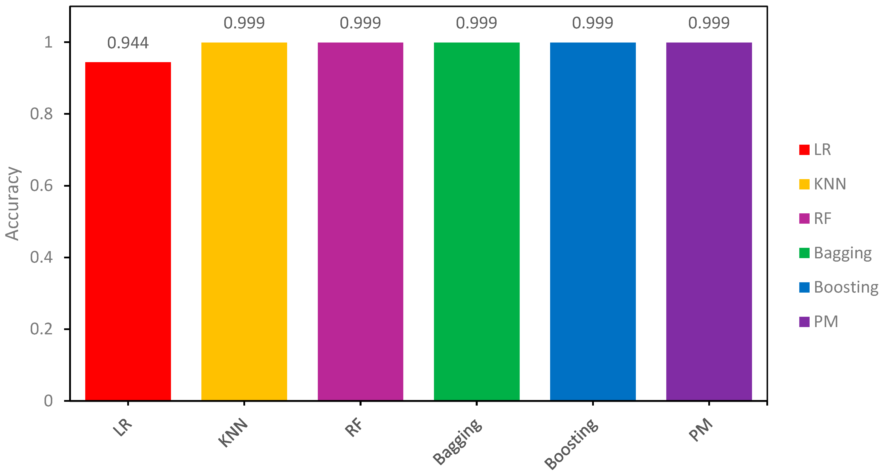
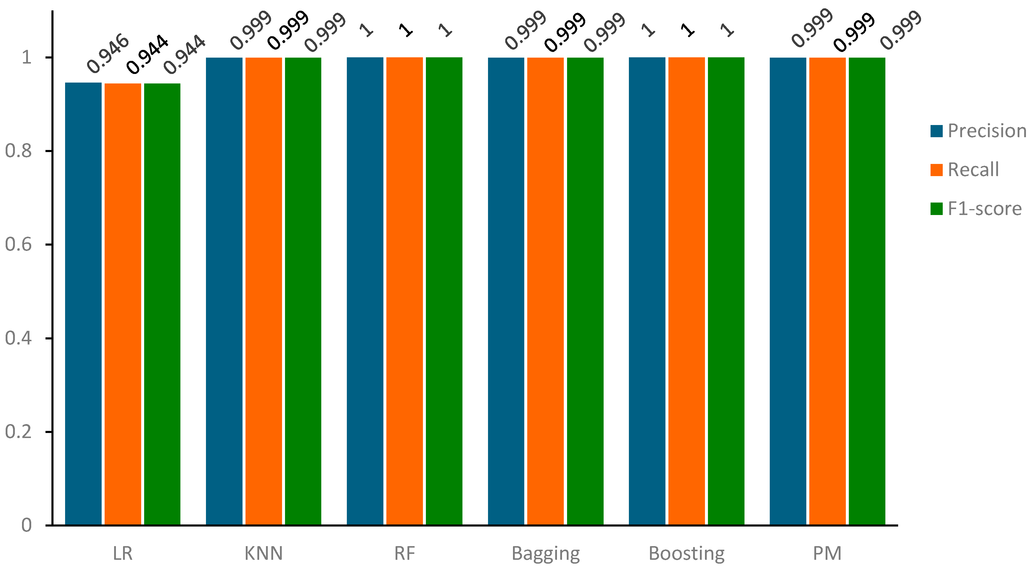
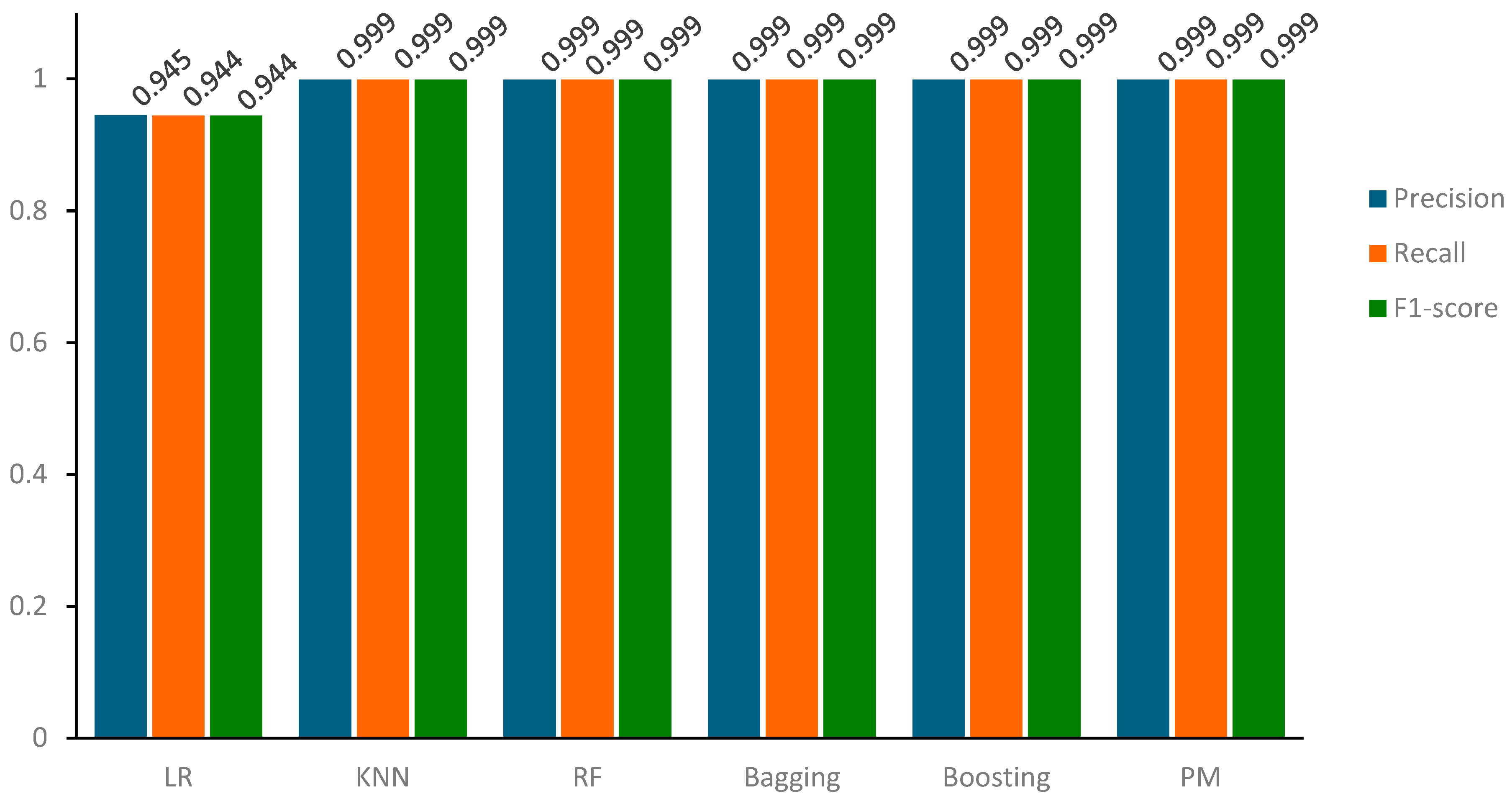
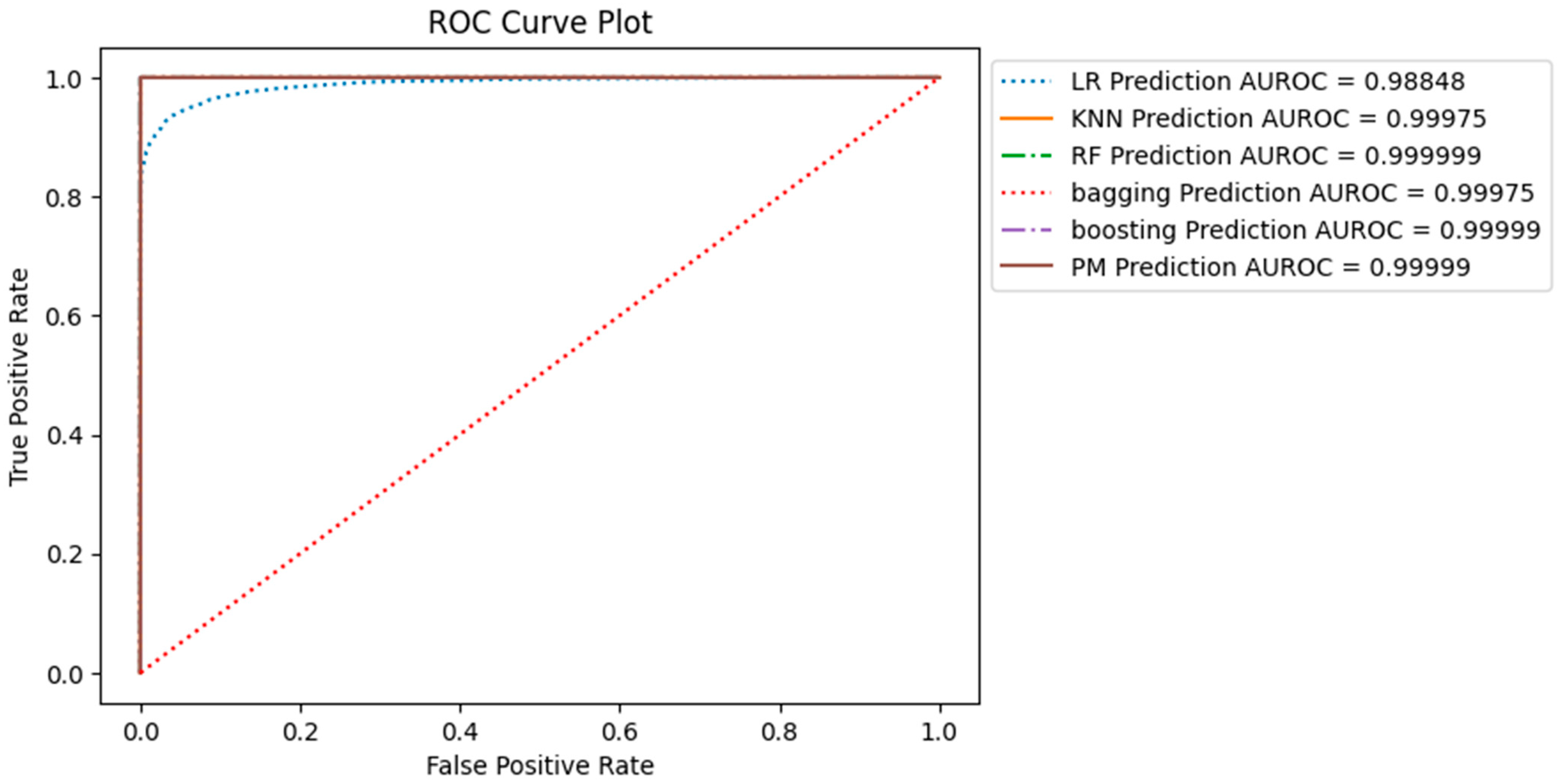
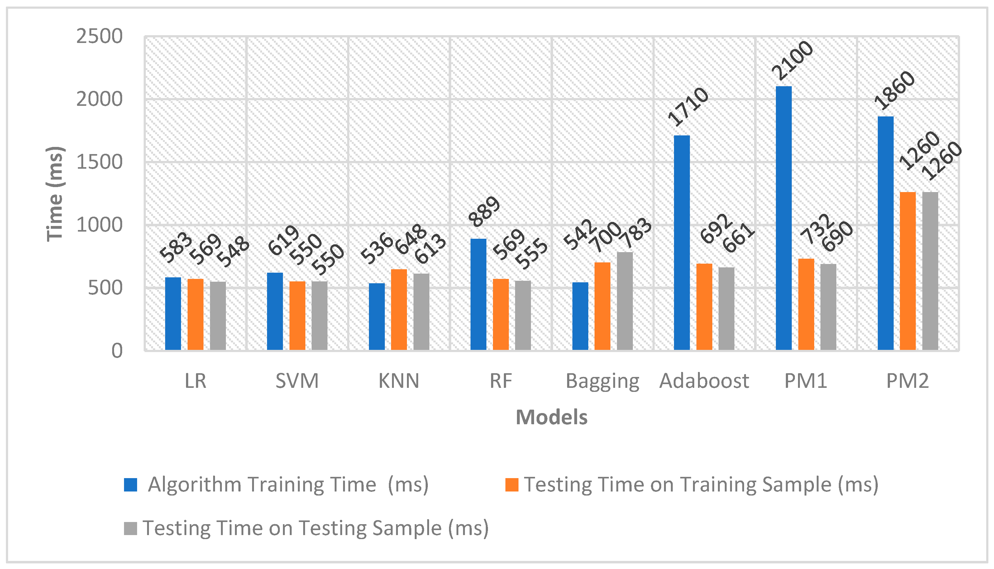
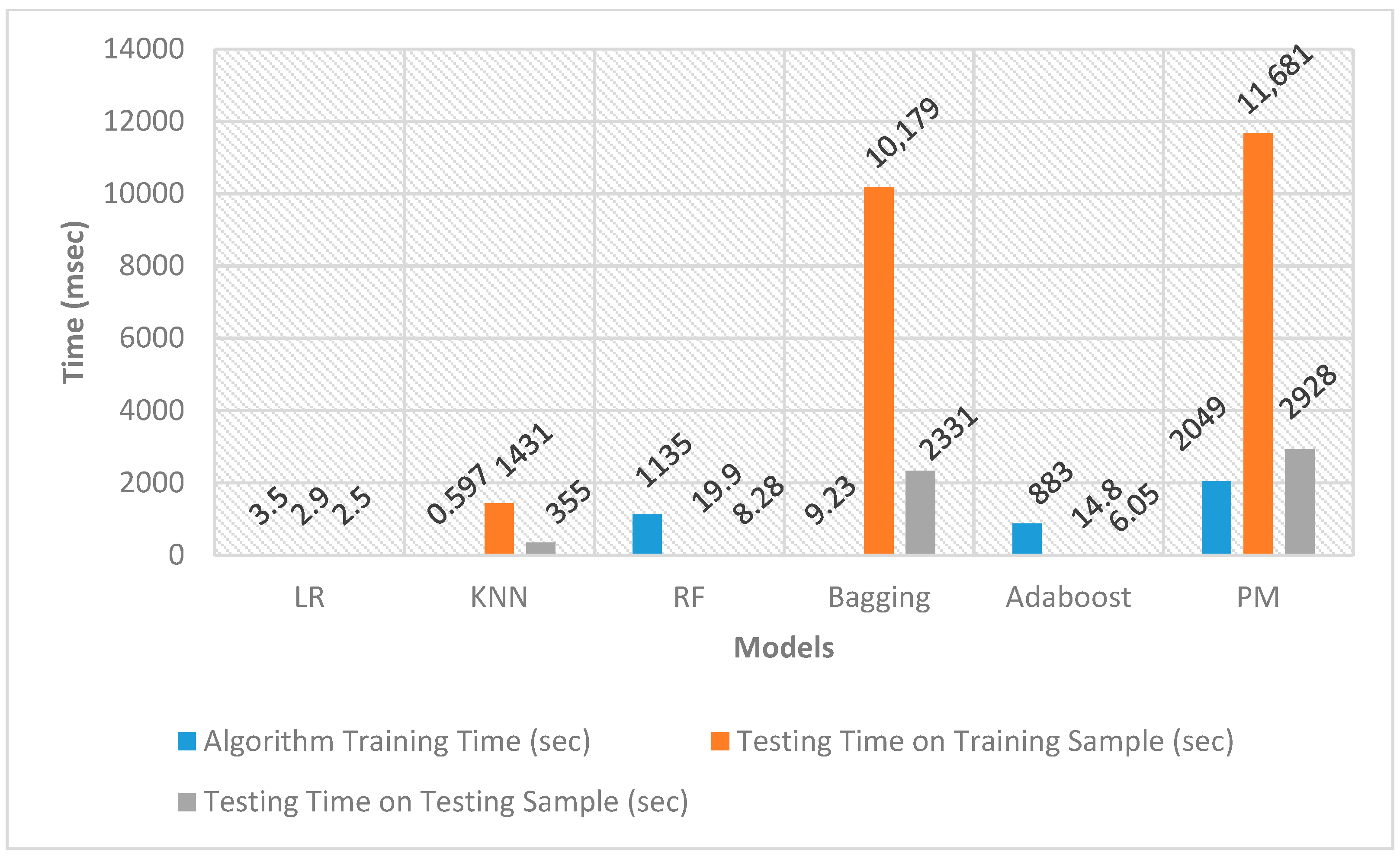
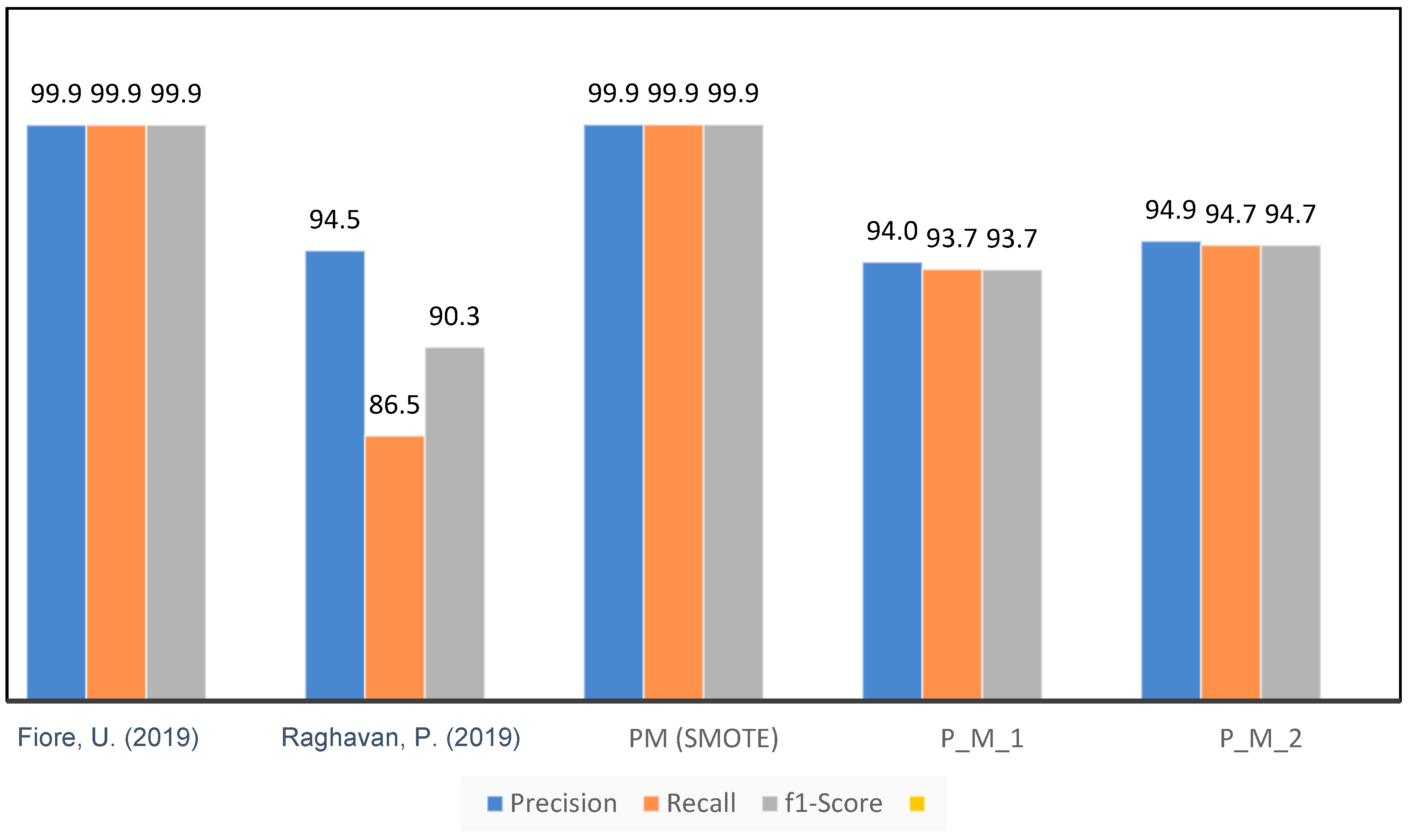
Table 1.
Comparison of ML Techniques Used in Credit Card Fraud Detection Research.
| Year | Authors | Ensemble ML Models | Under-Sampling | SMOTE | Comprehensive Evaluation |
|---|---|---|---|---|---|
| 2019 | Naik et al. [31] | ✓ | ✓ | × | ✓ |
| 2019 | Jain et al. [30] | ✓ | ✓ | × | ✓ |
| 2019 | Saputra et al. [29] | ✓ | × | ✓ | ✓ |
| 2019 | Raghavan et al. [28] | ✓ | × | ✓ | × |
| 2019 | Sadgali et al. [27] | ✓ | × | ✓ | × |
| 2020 | Sailusha et al. [26] | ✓ | × | ✓ | × |
| 2021 | Forough et al. [8] | ✓ | × | ✓ | × |
| 2021 | Tanouz et al. [25] | ✓ | ✓ | × | ✓ |
| 2022 | Qaddoura et al. [24] | ✓ | ✓ | ✓ | ✓ |
| 2022 | Sahithi et al. [1] | ✓ | × | ✓ | × |
| 2022 | Karthik et al. [9] | ✓ | × | ✓ | × |
| 2022 | Esenogho et al. [32] | ✓ | ✓ | ✓ | × |
| 2023 | Prasad et al. [23] | ✓ | ✓ | × | ✓ |
| 2023 | Our Proposed Model | ✓ | ✓ | ✓ | ✓ |
Table 2.
Confusion Matrix values for the Training sample.
| SVM | KNN | RF | Bagging | Boosting | P_M_1 | LR | P_M_2 | |
|---|---|---|---|---|---|---|---|---|
| True Positive | 345 | 345 | 378 | 344 | 378 | 354 | 349 | 358 |
| True Negative | 372 | 372 | 378 | 371 | 378 | 378 | 371 | 378 |
| False Positive | 33 | 33 | 0 | 34 | 0 | 24 | 29 | 20 |
| False Negative | 6 | 6 | 0 | 7 | 0 | 0 | 7 | 0 |
Table 3.
Confusion Matrix values for the Testing Sample.
| SVM | KNN | RF | Bagging | Boosting | P_M_1 | LR | P_M_2 | |
|---|---|---|---|---|---|---|---|---|
| True Positive | 87 | 86 | 86 | 87 | 86 | 85 | 87 | 87 |
| True Negative | 92 | 92 | 93 | 93 | 92 | 93 | 90 | 93 |
| False Positive | 8 | 9 | 9 | 8 | 9 | 10 | 8 | 8 |
| False Negative | 3 | 3 | 2 | 2 | 3 | 2 | 5 | 2 |
Table 4.
Accuracy results of all Models for the Training and Testing Sample Datasets.
| Training Sample of Under-Sample Dataset | ||||||||
|---|---|---|---|---|---|---|---|---|
| SVM | KNN | RF | Bagging | Boosting | P_M_1 | LR | P_M_2 | |
| Accuracy | 0.96 | 0.951 | 1 | 0.95 | 1 | 0.97 | 0.955 | 0.97 |
| Testing Sample of Under-Sample Dataset | ||||||||
| Accuracy | 0.9421 | 0.9368 | 0.937 | 0.9473 | 0.9368 | 0.9368 | 0.9315 | 0.9473 |
Table 5.
Precision, Recall, and F1-score of all Models for the Training Sample Dataset.
| SVM | KNN | RF | Bagging | Boosting | P_M_1 | LR | P_M_2 | |
|---|---|---|---|---|---|---|---|---|
| Precision | 0.961 | 0.955 | 1 | 0.953 | 1 | 0.971 | 0.957 | 0.971 |
| Recall | 0.96 | 0.951 | 1 | 0.95 | 1 | 0.97 | 0.955 | 0.97 |
| F1-score | 0.96 | 0.951 | 1 | 0.95 | 1 | 0.97 | 0.955 | 0.97 |
Table 6.
Precision, Recall, and F1-score of all Models for the Testing Sample of the Under-Sample Dataset.
Table 6.
Precision, Recall, and F1-score of all Models for the Testing Sample of the Under-Sample Dataset.
| SVM | KNN | RF | Bagging | Boosting | P_M_1 | LR | P_M_2 | |
|---|---|---|---|---|---|---|---|---|
| Precision | 0.942 | 0.945 | 0.939 | 0.939 | 0.945 | 0.945 | 0.948 | 0.949 |
| Recall | 0.942 | 0.942 | 0.937 | 0.937 | 0.942 | 0.942 | 0.947 | 0.947 |
| F1-score | 0.942 | 0.942 | 0.937 | 0.937 | 0.942 | 0.942 | 0.947 | 0.947 |
Table 7.
Confusion Matrix of all Models for the Training Sample of the SMOTE Dataset.
| LR | KNN | RF | Bagging | Boosting | P_M | |
|---|---|---|---|---|---|---|
| True Positive | 201,231 | 220,152 | 220,152 | 220,152 | 220,152 | 220,152 |
| True Negative | 214,606 | 219,868 | 220,152 | 219,864 | 220,152 | 220,082 |
| False Positive | 18,921 | 0 | 0 | 0 | 0 | 0 |
| False Negative | 5546 | 284 | 0 | 288 | 0 | 70 |
Table 8.
Confusion Matrix of all Models for the Testing Sample of the SMOTE Dataset.
| LR | KNN | RF | Bagging | Boosting | P_M | |
|---|---|---|---|---|---|---|
| True Positive | 50,280 | 55,038 | 55,038 | 55,038 | 55,038 | 55,038 |
| True Negative | 53,660 | 54,947 | 55,028 | 54,941 | 55,028 | 54,993 |
| False Positive | 4758 | 0 | 0 | 0 | 0 | 0 |
| False Negative | 1378 | 91 | 10 | 97 | 10 | 45 |
Table 9.
Accuracy Results of all Models for the Training Sample of the SMOTE Dataset.
| Training Sample of SMOTE Dataset | ||||||
|---|---|---|---|---|---|---|
| LR | KNN | RF | Bagging | Boosting | PM | |
| Accuracy | 0.94443 | 0.999354 | 1 | 0.9993 | 1 | 0.99983 |
| Testing Sample of SMOTE Dataset | ||||||
| Accuracy | 0.944256 | 0.999173 | 0.99989 | 0.999 | 0.999092 | 0.9996 |
Table 10.
Precision, Recall, and F1-score of all models for the Training sample of the SMOTE dataset.
Table 10.
Precision, Recall, and F1-score of all models for the Training sample of the SMOTE dataset.
| Prediction Results on the Training Sample of the SMOTE Dataset | ||||||
|---|---|---|---|---|---|---|
| LR | KNN | RF | Bagging | Boosting | PM | |
| Precision | 0.94607 | 0.999355 | 1 | 0.9993 | 1 | 0.99983 |
| Recall | 0.94443 | 0.99954 | 1 | 0.9993 | 1 | 0.999831 |
| F1-score | 0.94438 | 0.99954 | 1 | 0.9993 | 1 | 0.999831 |
Table 11.
Precision, Recall, and Accuracy of all models for the Testing Sample of the SMOTE dataset.
Table 11.
Precision, Recall, and Accuracy of all models for the Testing Sample of the SMOTE dataset.
| LR | KNN | RF | Bagging | Boosting | PM | |
|---|---|---|---|---|---|---|
| Precision | 0.945938 | 0.999174 | 0.999891 | 0.999 | 0.999092 | 0.999601 |
| Recall | 0.944256 | 0.999173 | 0.99989 | 0.999 | 0.999092 | 0.9996 |
| F1-score | 0.944204 | 0.999173 | 0.99989 | 0.999 | 0.999092 | 0.9996 |
Table 12.
Computational efficiency of all models for under-sampled and SMOTE datasets.
| Algorithm Training | Testing on Training Sample | Testing on Testing Sample | ||||
|---|---|---|---|---|---|---|
| Time (ms) | Memory Usage (MiB) | Time (ms) | Memory Usage (MiB) | Time (ms) | Memory Usage (MiB) | |
| LR | 583 | 1404.43–1403.46 | 569 | 1403.46–1403.46 | 548 | 1403.46–1403.46 |
| SVM | 619 | 1403.37–1403.37 | 550 | 1403.37–1403.37 | 550 | 1403.37–1403.39 |
| KNN | 536 | 1403.39 -1403.39 | 648 | 1403.39–1403.66 | 613 | 1403.66–1403.66 |
| RF | 889 | 1403.66–1403.90 | 569 | 1403.90–1403.90 | 555 | 1403.90–1403.90 |
| Bagging | 542 | 1403.90–1403.90 | 700 | 1403.90–1403.90 | 783 | 1403.90–1403.91 |
| Adaboost | 1710 | 1403.91–1403.91 | 692 | 1403.91–1403.91 | 661 | 1403.91–1403.91 |
| PM1 | 2100 | 1403.91–1403.91 | 732 | 1403.91–1403.91 | 690 | 1403.91–1403.91 |
| PM2 | 1860 | 1404.47–1403.47 | 1260 | 1404.47–1403.47 | 1260 | 1404.47–1403.47 |
| SMOTE Dataset | ||||||
| LR | 3.5 | 1190.03–1190.64 | 2.9 | 1190.65–1190.65 | 2.5 | 1190.77–1190.77 |
| KNN | 0.597 | 1190.77–1288.20 | 1431 | 1288.20–1295.43 | 355 | 1295.43–1295.89 |
| RF | 1135 | 1295.93–1296.31 | 19.9 | 1296.31–1296.31 | 8.28 | 1296.31–1296.33 |
| Bagging | 9.23 | 1147.86–1841.64 | 10,179 | 1841.89–819.89 | 2331 | 820.93–1342.43 |
| Adaboost | 883 | 1341.71–1454.40 | 14.8 | 1454.46–1458.23 | 6.05 | 1456.50–1456.86 |
| PM | 2049 | 1455.36–2282.86 | 11,681 | 2282.89–2158.89 | 2928 | 2155.05–2028.86 |
Disclaimer/Publisher’s Note: The statements, opinions and data contained in all publications are solely those of the individual author(s) and contributor(s) and not of MDPI and/or the editor(s). MDPI and/or the editor(s) disclaim responsibility for any injury to people or property resulting from any ideas, methods, instructions or products referred to in the content. |
© 2024 by the authors. Licensee MDPI, Basel, Switzerland. This article is an open access article distributed under the terms and conditions of the Creative Commons Attribution (CC BY) license (https://creativecommons.org/licenses/by/4.0/).
Share and Cite
MDPI and ACS Style
Khalid, A.R.; Owoh, N.; Uthmani, O.; Ashawa, M.; Osamor, J.; Adejoh, J. Enhancing Credit Card Fraud Detection: An Ensemble Machine Learning Approach. Big Data Cogn. Comput. 2024, 8, 6. https://doi.org/10.3390/bdcc8010006
AMA Style
Khalid AR, Owoh N, Uthmani O, Ashawa M, Osamor J, Adejoh J. Enhancing Credit Card Fraud Detection: An Ensemble Machine Learning Approach. Big Data and Cognitive Computing. 2024; 8(1):6. https://doi.org/10.3390/bdcc8010006
Chicago/Turabian StyleKhalid, Abdul Rehman, Nsikak Owoh, Omair Uthmani, Moses Ashawa, Jude Osamor, and John Adejoh. 2024. "Enhancing Credit Card Fraud Detection: An Ensemble Machine Learning Approach" Big Data and Cognitive Computing 8, no. 1: 6. https://doi.org/10.3390/bdcc8010006