The Fractal Nature of an Approximate Prime Counting Function

Abstract

Prime number related fractal polygons and curves are derived by combining two different aspects. One is an approximation of the prime counting function build on an additive function. The other is prime number indexed basis entities taken from the discrete or continuous Fourier basis.

1. Introduction

The present work describes the results of a numerical experiment based on the approximate prime counting function presented in [1]. By searching for a visual representation for the distribution of primes different to the well known staircase plots of the prime counting function, the authors used regular polygons and their relation to prime numbers as described in [2]. In doing so, fractal polygons and curves have been derived which will be presented in the following.

The distribution of prime numbers is one of the central problems in analytic number theory. Here, the prime counting function $\pi \left(x\right)$, giving the number of primes less or equal to $x\in \mathbb{R}$, is of special interest. As stated in [3]: when the large-scale distribution of primes is considered, it appears in many ways quite regular and obeys simple laws. One of the first central results regarding the asymptotic distribution of primes is given by the prime number theorem, providing the limit

$$\underset{x\to \infty }{lim}\frac{\pi \left(x\right)}{x/lnx}=1,$$

(1)

which was proved independently in 1896 by Jacques Salomon Hadamard and Charles-Jean de La Vallée Poussin. Both proofs are based on complex analysis using the Riemann zeta function $\zeta \left(s\right):={\sum }_{n=1}^{\infty }1/n^s$, with $s\in \mathbb{C}$ and the fact that $\zeta \left(s\right)\ne 0$ for all $s:=1+\mathrm{i}y$, $y>0$.

An improved approximation of $\pi \left(x\right)$ is given by the Eulerian logarithmic integral

$$Li\left(x\right):={\int }_2^x\frac{\mathrm{d}t}{lnt}.$$

(2)

This result was first mentioned by Carl Friedrich Gauß in 1849 in a letter to Encke refining the estimate $n/ln\left(n\right)$ of $\pi \left(n\right)$ given by the only 15 years old Gauß in 1792. This conjecture was also stated by Legendre in 1798.

In 2007 Terence Tao gave an informal sketch of proof in his lecture “Structure and randomness in the prime numbers” as follows [4]:

• Create a “sound wave” (or more precisely, the von Mangoldt function) which is noisy at prime number times, and quiet at other times. [...]
• “Listen” (or take Fourier transforms) to this wave and record the notes that you hear (the zeroes of the Riemann zeta function, or the “music of the primes”). Each such note corresponds to a hidden pattern in the distribution of the primes.

In the same spirit, the present work tries to paint a picture of the primes. By combining an alternative approximation of the prime counting function $\pi \left(x\right)$ based on an additive function as proposed in [1] with prime number related Fourier polygons used in the context of regularizing polygon transformations as given in [2,5], fractal prime polygons and fractal prime curves are derived.

Three types of structures in the distribution of prime numbers are distinguished in [6]. The first is local structure, like residue classes or arithmetic progression [7]. The second is asymptotic structure as provided by the prime number theorem. The third is statistical structure as described for example in [8] reporting an empirical evidence of fractal behavior in the distribution of primes or [9] describing fractal fluctuations in the spacing intervals of adjacent prime numbers generic to diverse dynamical systems in nature. Quasi self similar structures in the distribution of differences of prime-indexed primes with scaling by prime-index order have been observed in [6]. The distribution of primes and prime-indexed primes is studied in [10] by mapping primes into a binary image. It is observed that the recurrence plots of prime distribution are similar to the Cantor dust. In the present work, the asymptotic structure becomes visually apparent by the given fractals.

2. Approximations of the Prime Counting Function

This section presents briefly the prime counting function and its classic approximations. Furthermore, an approximate prime counting function based on an additive function is described which yields the starting point in deriving prime related fractals.

Let $\mathbb{N}:=\{1,2,3,\cdots \}$ denote the set of natural numbers, ${\mathbb{N}}_0:=\mathbb{N}\cup \left\{0\right\}$, and $p_k$ the kth prime number with $k\in \mathbb{N}$, i.e., $p_1$ := 2, $p_2$ := 3, $p_3$ := 5, etc. For $x\in \mathbb{R}$, the prime counting function is defined as

$$\pi \left(x\right):=\left\{\begin{array}{ll}0\hfill & \mathrm{if}x<2,\hfill \\ max\{k\in \mathbb{N}|p_k\le x\}\hfill & \mathrm{else}.\hfill \end{array}\right.$$

(3)

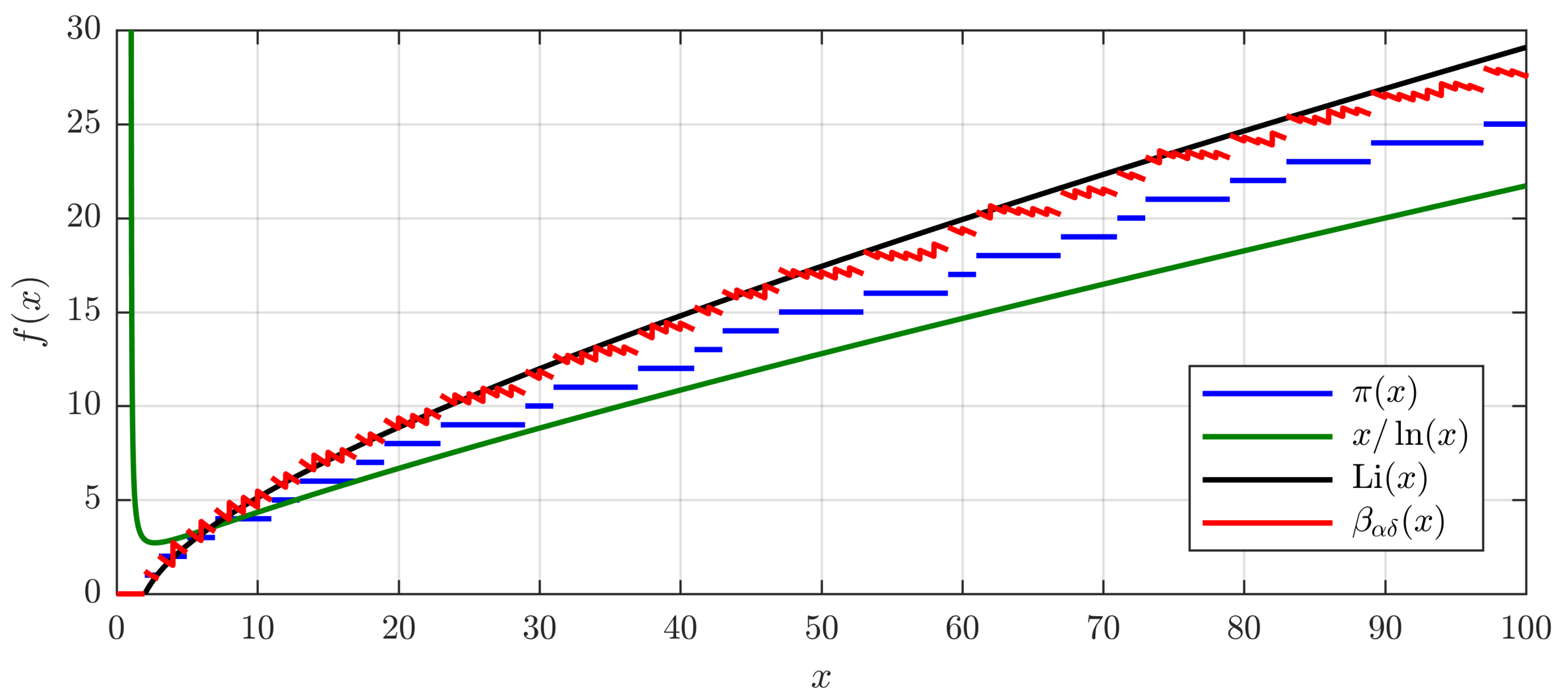
According to the prime number theorem, $\pi \left(x\right)$ can be approximated by $x/ln\left(x\right)$, i.e., (1) holds which will be denoted as $\pi \left(x\right)\sim x/ln\left(x\right)$. An improved approximation is given by the Eulerian logarithmic integral (2), i.e., $\pi \left(x\right)\sim Li\left(x\right)$. The graphs of the prime counting function and its two approximations are depicted in Figure 1 for $x\in [0,100]$.

An alternative approximation of $\pi \left(x\right)$ is proposed in [1]. Its definition is based on an additive function which will be given in the following. Each $n\in \mathbb{N}\setminus \left\{1\right\}$ can be written as prime factorization $n={\prod }_{k\in I\left(n\right)}{p}_k^{{\alpha }_k\left(n\right)}$ with the prime numbers $p_k$ and their associated multiplicities ${\alpha }_k\left(n\right)\in \mathbb{N}$. Here, $I\left(n\right)$ denotes the index set of the prime numbers which are part of the factorization of n. For example, for $50=2^1·5^2$ it holds that $I\left(n\right)=\{1,3\}$ and ${\alpha }_1\left(50\right)=1$, ${\alpha }_3\left(50\right)=2$.

An additive function ${\beta }_{\alpha }:\mathbb{N}\to {\mathbb{N}}_0$ is given by the sum of all prime factors multiplied by their associated multiplicities, i.e.,

$${\beta }_{\alpha }\left(n\right):=\left\{\begin{array}{cc}0\hfill & \mathrm{for}n=1,\hfill \\ {\sum }_{k\in I\left(n\right)}{\alpha }_k\left(n\right)p_k\hfill & \mathrm{otherwise}.\hfill \end{array}\right.$$

(4)

Here, additive function means that $n_1,n_2\in \mathbb{N}$ implies ${\beta }_{\alpha }\left(n_1{n}_2\right)={\beta }_{\alpha }\left(n_1\right)+{\beta }_{\alpha }\left(n_2\right)$. Furthermore, for prime numbers it follows readily that ${\beta }_{\alpha }\left(p_k\right)=p_k$, $k\in \mathbb{N}$. The arithmetic properties of the function ${\beta }_{\alpha }\left(n\right)$ are discussed in [11]. Here, this function, also known as integer logarithm, is denoted as $A\left(n\right)$.

Summing ${\beta }_{\alpha }\left(n\right)$ for all n less or equal to a given real number $x>0$ and applying proper scaling leads to the definition of

$${\beta }_{\alpha \delta }\left(x\right):=\frac{12}{{\pi }^{2}x}\sum _{n\in \mathbb{N},n\le x}{\beta }_{\alpha }\left(n\right).$$

(5)

The graph of ${\beta }_{\alpha \delta }\left(x\right)$ is depicted red in Figure 1. As a central result, it has been shown in [1] that ${\beta }_{\alpha \delta }\left(x\right)\sim \pi \left(x\right)$ which is due to the representation

$$B_{\alpha }\left(x\right):=\sum _{n\in \mathbb{N},n\le x}{\beta }_{\alpha }\left(n\right)=\frac{{\pi }^2}{12}\frac{x^2}{lnx}+\mathcal{O}\left(\frac{x^2}{{ln}^{2}x}\right).$$

(6)

This approximation of the prime counting function provides the first ingredient for deriving prime related fractals. The second ingredient is given by the following section.

3. Polygon Transformations and Fourier Polygons

Regular polygons and their relation to prime numbers are described in [2] in the context of regularizing polygon transformations. Such transformations, also generalized in [5], are based on constructing similar triangles on the sides of the polygon to transform. By iteratively applying the transformation, regular polygons are obtained for specific choices of the transformation parameters. Here, a point of a planar polygon can be represented by a complex number, the polygon itself by a vector of complex numbers. As is described briefly in this section, regularizing transformations can be represented by circulant matrices. Hence they are diagonalizable by the discrete Fourier matrix and the limit polygons are linear combinations of column vectors of the discrete Fourier matrix. These column vectors represent regular polygons which are denoted as Fourier polygons. This section gives a short introduction to regularizing polygon transformations and the theoretical background which builds the foundation for a specific choice of basis functions in finding an alternative geometric representation for visualizing polygons and curves related to the distribution of primes.

For a given $n\in \mathbb{N}$, $n\ge 3$, let $z={(z_0,\cdots ,z_{n-1})}^{\mathrm{t}}\in {\mathbb{C}}^n$ denote an arbitrary polygon in the complex plane. In the following, all indices have to be taken modulo n. In the first transformation substep, the similar triangles constructed on each directed side $z_k{z}_{k+1}$, $k\in \{0,\cdots ,n-1\}$, of the polygon are parameterized by a prescribed side subdivision ratio $\lambda \in (0,1)$ and a base angle $\theta \in (0,\pi /2)$. This is done by constructing the perpendicular to the right of the side at the subdivision point $\lambda z_k+(1-\lambda )z_{k+1}$. On this perpendicular, a new polygon vertex $z_{k+1}^{\prime }$ is chosen in such a way that the triangle side $z_k{z}_{k+1}^{\prime }$ and the polygon side $z_k{z}_{k+1}$ enclose the prescribed angle $\theta$. 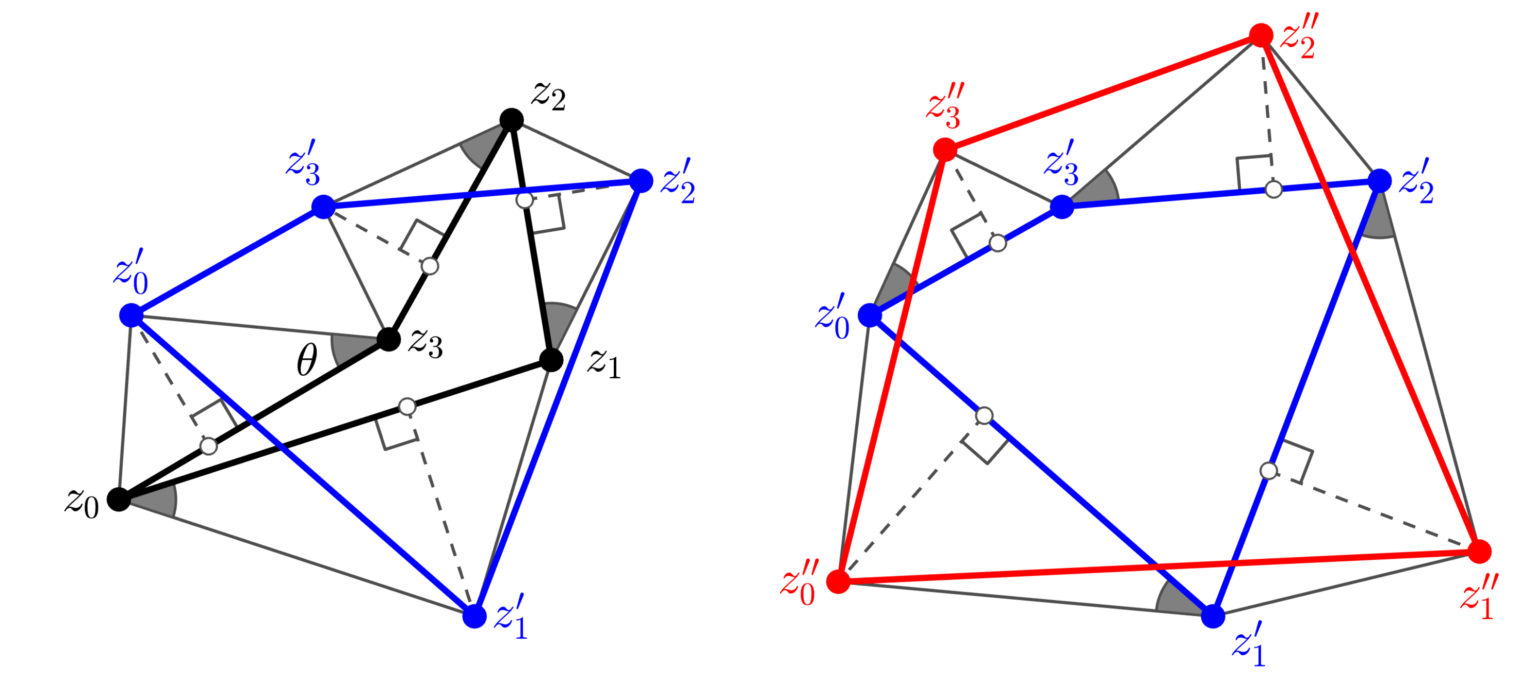This is depicted on the left side of Figure 2 for an initial polygon with vertices $z_k$ marked black. The construction of the first transformation substep leads to a new polygon with vertices $z_k^{\prime }$ marked blue. The subdivision points, located on the edges of the initial polygon, are marked by white circles, the associated perpendiculars by dashed lines, and the angles $\theta$ by grey arcs. In the given example, the transformation parameters have been set to $\lambda =1/3$ and $\theta =\pi /5$.

The rotational effect of the first transformation substep is compensated by applying a second transformation substep with flipped similar triangles as is depicted on the right side of Figure 2. Starting from the vertices $z_k^{\prime }$ of the first transformation substep marked blue, this results in the polygon with vertices $z_k^{″}$ depicted red. As has been shown in [5], for $w:=\lambda +\mathrm{i}(1-\lambda )tan\theta$, the new polygon vertices obtained by applying these two substeps are given by

$$z_{k+1}^{\prime }:=w{z}_k+(1-w)z_{k+1}\mathrm{and}{z}_k^{″}:=(1-\overline{w})z_k^{\prime }+\overline{w}{z}_{k+1}^{\prime },$$

respectively, where $\overline{w}$ denotes the complex conjugate of w. Both substeps are linear mappings in ${\mathbb{C}}^n$ and the combined mapping is given by the matrix representation

$$z^{″}=Mz,\mathrm{where}{M}_{j,k}:=\left\{\begin{array}{cc}{|1-w|}^2+{\left|w\right|}^2\hfill & \mathrm{if}j=k,\hfill \\ w(1-\overline{w})\hfill & \mathrm{if}j=k+1,\hfill \\ \overline{w}(1-w)\hfill & \mathrm{if}k=j+1,\hfill \\ 0\hfill & \mathrm{otherwise},\hfill \end{array}\right.$$

(7)

with $j,k\in \{0,\cdots ,n-1\}$.

The transformation matrix M is circulant and Hermitian [5]. Hence, with $r:=exp(2\pi \mathrm{i}/n)$ denoting the nth root of unity, it holds that M is diagonalized by the $n\times n$ unitary discrete Fourier matrix

$$F:=\frac{1}{\sqrt{n}}\left(\begin{array}{ccc}{r}^{0·0}& \cdots & r^{0·(n-1)}\\ ⋮& \ddots & ⋮\\ r^{(n-1)·0}& \cdots & r^{(n-1)·(n-1)}\end{array}\right)$$

(8)

with entries $F_{j,k}=r^{jk}/\sqrt{n}$ and zero-based indices $j,k\in \{0,\cdots ,n-1\}$ [12].

Let $z^{\left(\ell \right)}:=M^{\ell }z$ denote the polygon obtained by applying the transformation ℓ times. If ℓ tends to infinity, the shape of the scaled limit polygon $z^{(\infty )}$ depends on the dominating eigenvalue of M and the associated column of F. In the following, such a kth column of F is denoted as the kth Fourier polygon, i.e.,

$$f_k:={\left(r^{0·k},\cdots ,r^{(n-1)·k}\right)}^{\mathrm{t}},k\in \{0,\cdots ,n-1\}.$$

(9)

Hence, the Fourier polygons are the prototypes of the limit polygons obtained by iteratively applying M. A full classification of these limit polygons with respect to the choice of the transformation parameters $\lambda$ and $\theta$ is given in [5]. Such transformations leading to regular polygons can for example be used in finite element mesh smoothing [13]. Furthermore, similar smoothing schemes can also be applied to volumetric meshes. Here, transformations can for example be based on geometric constructions [14] or on the gradient flow of the mean volume [15].

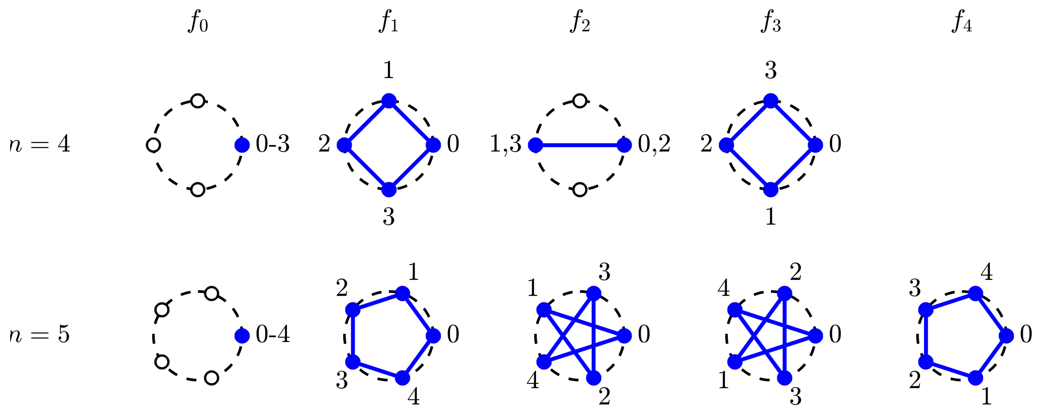
For $n=4$, the four Fourier polygons are depicted in the upper row of Figure 3. Since the jth vertex of $f_k$ is the $jk$th power of r, $f_0$ consists of four times the vertex $1+0\mathrm{i}$, as is indicated by the blue point and the vertex label 0–3. The unit circle is marked by a dashed line, the roots of unity by white circle markers. As can be seen, $f_1$ is the regular counterclockwise oriented quadrilateral, $f_2$ a doubled segment with vertex multiplicity two.

In contrast to the case $n=4$, there is no degenerate polygon in the case $n=5$ except that for $k=0$, as is shown in the lower row of Figure 3. Since the kth Fourier polygon is derived by iteratively connecting each kth vertex defined by the unit roots, and $n=5$ is a prime number, each polygon vertex has multiplicity one. That is, in the case of prime numbers, all $f_k$ are either regular n-gons or star shaped n-gons if $k>0$. This relation between iterative polygon transformation limits and prime numbers is also analyzed in [2]. Furthermore, the roots of unity form a cyclic group under multiplication. For a given number n and each prime number $p\le n$, there is an associated Fourier polygon $f_{p-1}$ defined by (9). This is the second ingredient in defining prime counting function related fractals.

4. Deriving Prime Fractals

The graph of the approximate prime counting function ${\beta }_{\alpha \delta }\left(x\right)$ depicted in Figure 1 gives only an impression for small values of x. Furthermore, it is not suitable to reveal more insight into the inner structure of prime numbers and their distribution. In search for such a graphical representation, a combination of the approximate prime counting function and Fourier polygons is considered in the following.

The main ingredient of the approximate prime counting function ${\beta }_{\alpha \delta }$ given by (5) is its scaled counterpart $B_{\alpha }\left(x\right)$ given by (6). For $x\in \mathbb{N}\setminus \left\{1\right\}$, this sum can be written as

$$B_{\alpha }\left(n\right)=\sum _{k=2}^n{\beta }_{\alpha }\left(k\right)=\sum _{k=2}^n\sum _{j\in I\left(k\right)}{\alpha }_j\left(k\right)p_j=\sum _{k\in \mathbb{N},p_k\le n}\underset{=:w_k\left(n\right)}{\underbrace{\left(\sum _{j=1}^{\lfloor {log}_{p_k}n\rfloor }⌊\frac{n}{p_k^j}⌋\right)}}{p}_k,$$

(10)

where $\lfloor ·\rfloor$ denotes the floor function. That is, $B_{\alpha }\left(n\right)$ is a weighted sum of prime numbers. The latter representation can be obtained by collecting all coefficients in the sum on the left side of (10) for each prime number $p_k$ using a sieve of Eratosthenes based argument.

The key to prime fractals is to replace the prime numbers $p_k$ in the representation of $B_{\alpha }\left(n\right)$ according to (10) by prime number associated Fourier polygons. This leads to the polygonal prime fractal

$$F_p\left(n\right):=\sum _{k\in \mathbb{N},p_k\le n}{w}_k\left(n\right)f_{p_k-1},$$

(11)

with $f_k$ denoting the Fourier polygon according to (9). Here, the Fourier polygon index $p_k-1$ consists of the kth prime number subtracted by one, since zero based indices are used in the discrete Fourier transformation scheme.

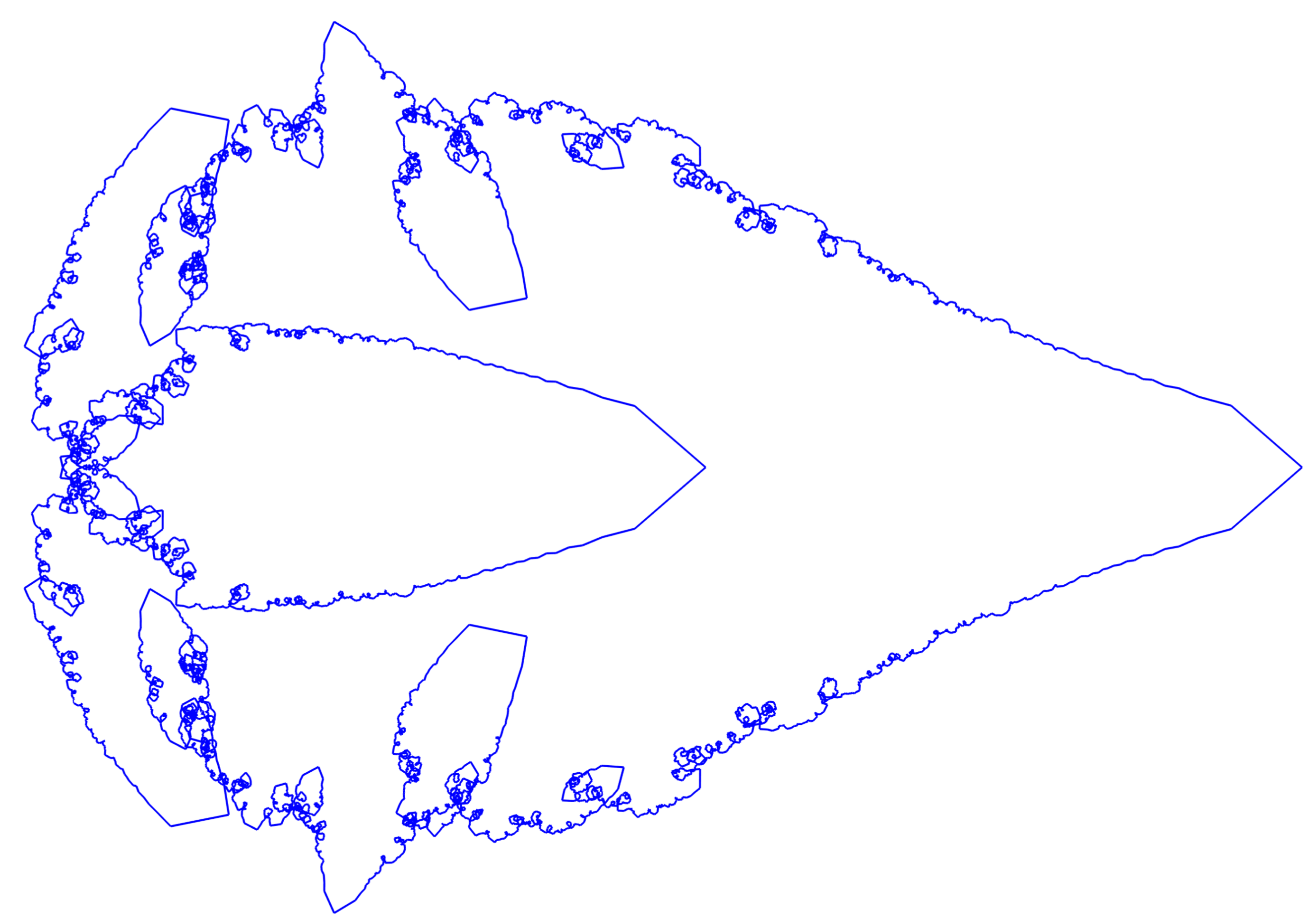
For $n={10}^4$, the polygonal prime fractal $F_p\left({10}^4\right)$ is depicted in Figure 4. It is a linear combination of $\pi \left({10}^4\right)=1229$ Fourier polygons $f_{p_k-1}$, each weighted with its associated coefficient $w_k\left(n\right)$ as defined in (10). This polygon consists of $n={10}^4$ vertices. The fractal structure of this polygon is already visible for this comparably low value of n. However, due to its discrete nature, self similarity is not that obvious for some parts of the polygon. Therefore, an improved fractal is derived by using the continuous Fourier basis instead of the discrete Fourier basis. That is, the Fourier polygon $f_k$ is replaced by the Fourier basis function $f_k\left(t\right):=exp\left(\mathrm{i}kt\right)$. 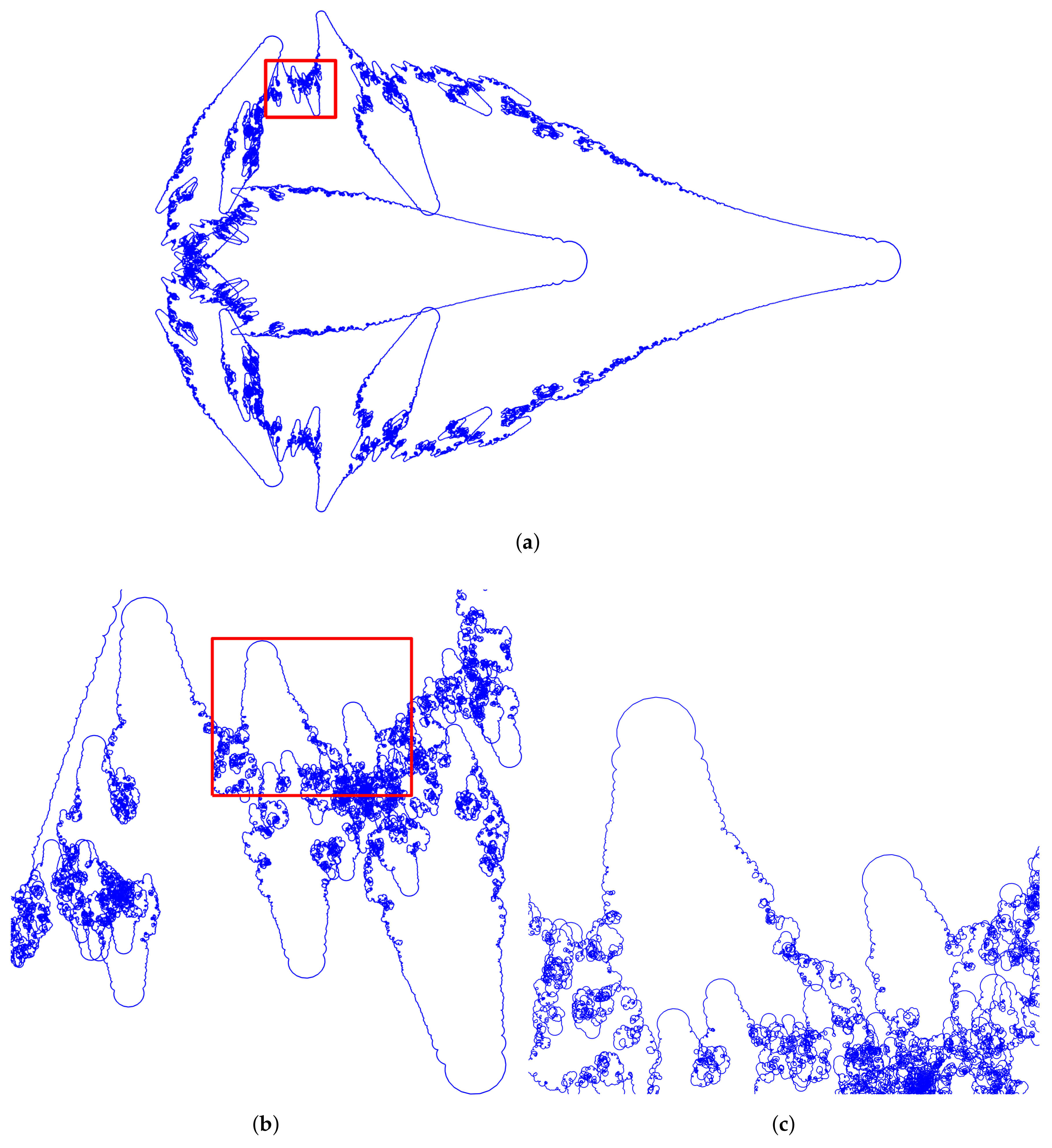This results in the prime fractal curve

$$F_c(n,t):=\sum _{k\in \mathbb{N},p_k\le n}{w}_k\left(n\right)exp\left(\mathrm{i}(p_k-1)t\right),\mathrm{with}t\in (-\pi ,\pi ].$$

(12)

For $n={10}^6$, the resulting prime fractal curve is depicted in Figure 5a. It has been obtained by evaluating $F_c({10}^6,t)$ at ${10}^7$ equidistant parameters $t\in (-\pi ,\pi ]$. In this case, $F_c$ is the sum of $\pi \left({10}^6\right)=78498$ weighted Fourier basis functions. A zoom of the box marked red in Figure 5a is depicted in Figure 5b. The recurring structures show the fractal nature of the curve.

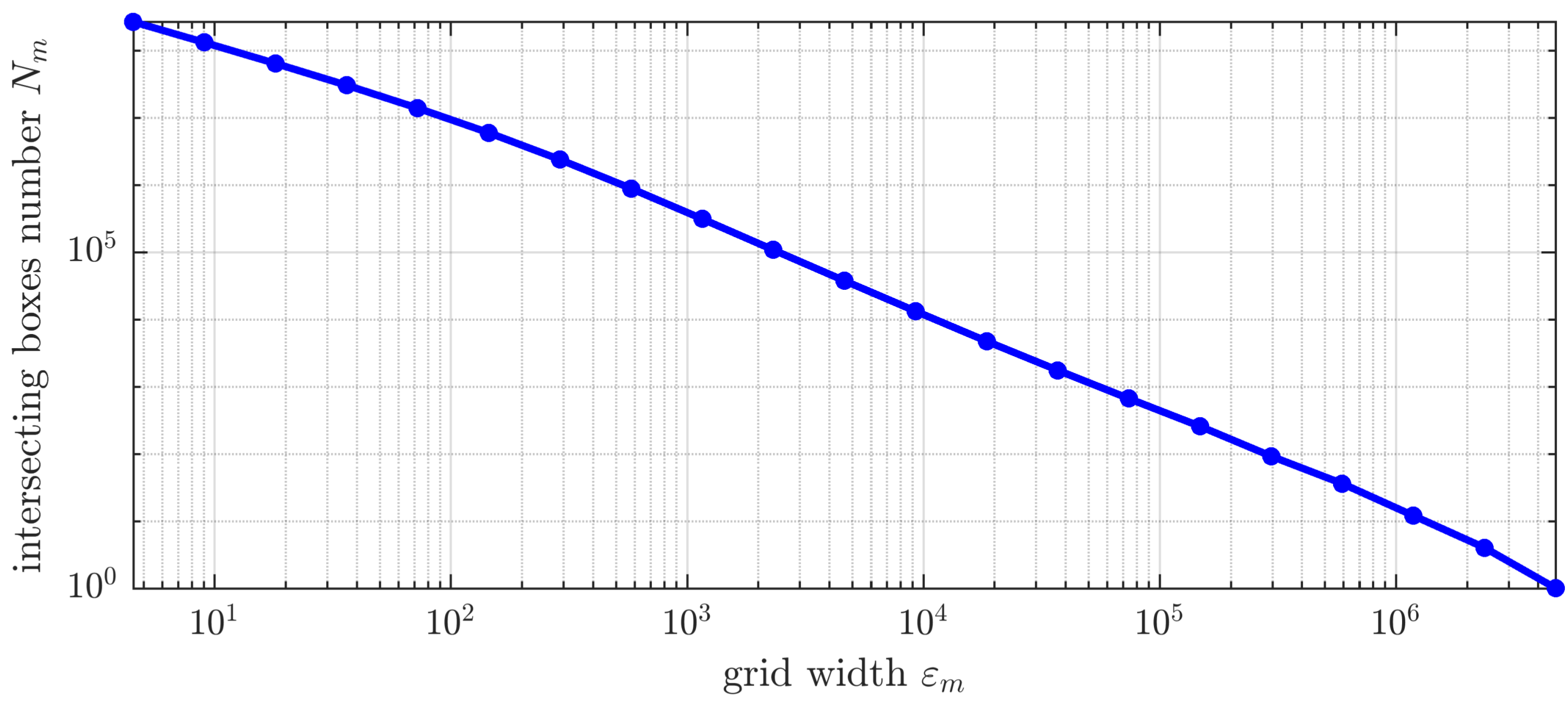
The fractal dimension of a curve, also known as Minkowski-Bouligand dimension, is given by

$$d:=\underset{\epsilon \to \infty }{lim}\frac{logN\left(\epsilon \right)}{log(1/\epsilon )},$$

(13)

where $\epsilon$ denotes the edge length of the square boxes covering the fractal curve and $N\left(\epsilon \right)$ the number of covering boxes [16]. For the curve depicted in Figure 5a, the fractal dimension is estimated by recursively subdividing a tight initial square bounding box of $F_c$. For each subdivision level $m\in \{0,\cdots ,20\}$, this results in a grid of $2^m\times 2^m$ squares and the associated estimate $d_m:=log\left(N_m\right)/log\left(2^m\right)$, where $N_m$ denotes the number of grid boxes with nonempty intersections with the fractal curve. The approximate fractal dimension for the finest subdivision grid results to $d_{20}\approx 1.3995$.

Figure 6 depicts the number of nonempty intersection boxes $N_m$ versus the grid width ${\epsilon }_m$ for $m\in \{0,\cdots ,20\}$ using logarithmic scales for both axes. The fractal dimension estimate derived by the slope of the line of best fit of these 21 points amounts to $d\approx 1.4107$.

5. Conclusions

In this publication, prime number related fractal polygons and curves have been derived by combining two different results. One is the approximation of the prime counting function $\pi \left(x\right)$ by the partial sum ${\beta }_{\alpha \delta }\left(x\right)$ based on an additive function as proposed in [1]. The other are prime indexed basis functions of the continuous Fourier transform. The motivation for this are the column vectors of the discrete Fourier matrix used for diagonalizing a circulant Hermitian matrix representing a regularizing transformation of polygons in the complex plane.

As has been shown in earlier publications [2,5], there is a relation between the shape of limit polygons of such iteratively applied polygon transformations and prime numbers. This is due to the cyclic group defined by the roots of unity and the exponential representation of the entries of the columns of the discrete Fourier matrix. The latter are called Fourier polygons. For prime number indices, these polygons are star shaped.

By replacing the prime numbers in a scaled representation of ${\beta }_{\alpha \delta }\left(x\right)$ for a given $x\in \mathbb{N}$ by the associated Fourier polygons, the polygonal prime fractal $F_p$ is derived. Its graphical features are increased, if x tends to infinity. Alternatively, by using the prime number related basis functions of the continuous Fourier transform, the prime fractal curve $F_c$ is derived which is approximated by $F_p$. The prime fractal polygon as well as the prime fractal curve show similar patterns on different scales as has been demonstrated graphically. In addition, a numerical estimate for the fractal dimension based on the box counting method was derived for the case $n={10}^6$. However, obtaining more detailed results for much larger n would be desirable.

The given result combines aspects from prime number theory, group theory, and circulant Hermitian matrices. It is based on Fourier transformation which also plays a role in dynamical systems associated to geometric element transformations [17]. The resulting prime fractals provide an alternative visual representation of an approximation of the prime counting function and with this of prime numbers and their structures itself. It is hoped that these alternative representations provide a basis for further insights into the structure of the distribution of prime numbers. Furthermore, applying similar visualization techniques to other number theory functions might reveal additional insights. This is also the subject of the subsequent publication [18] analyzing fractal curves from prime trigonometric series and the distribution of prime numbers.