A Fractional B-spline Collocation Method for the Numerical Solution of Fractional Predator-Prey Models


Department of Basic and Applied Sciences for Engineering (SBAI), University of Roma “La Sapienza”, Via Antonio Scarpa 16, 00161 Roma, Italy
Fractal Fract. 2018, 2(1), 13; https://doi.org/10.3390/fractalfract2010013
Submission received: 22 December 2017
/
Revised: 12 February 2018
/
Accepted: 12 February 2018
/
Published: 17 February 2018
(This article belongs to the Special Issue Fractional Dynamics)
Abstract
:We present a collocation method based on fractional B-splines for the solution of fractional differential problems. The key-idea is to use the space generated by the fractional B-splines, i.e., piecewise polynomials of noninteger degree, as approximating space. Then, in the collocation step the fractional derivative of the approximating function is approximated accurately and efficiently by an exact differentiation rule that involves the generalized finite difference operator. To show the effectiveness of the method for the solution of nonlinear dynamical systems of fractional order, we solved the fractional Lotka-Volterra model and a fractional predator-pray model with variable coefficients. The numerical tests show that the method we proposed is accurate while keeping a low computational cost.
1. Introduction
Fractional Calculus generalizes to real order the well known concept of derivative and integral of integer order. Even if the birth of fractional calculus can be set at the beginning of the 18th century, its use for the modeling of real-life problems is very recent. Nevertheless, in the last decades the interest in fractional differential and integral equations is rapidly growing and models involving fractional derivatives and/or integrals are widely used in several fields, from physics to continuum mechanics, from biophysics to electro-chemistry, from signal processing to control theory. For an introduction to fractional calculus see, for instance, [1,2,3,4] while a survey on its applications can be found in [5,6,7,8,9].
The reason why the fractional derivative is more suitable to model real-world problems is related to its non-local behavior that is able to introduce in a elegant way into the model, either memory effects in time or non-locality in space. In this paper we refer to the traditional Caputo fractional derivative introduced in [10] and extensively used to model a great variety of mechanical and biological phenomena. More recently, new fractional derivatives having non-singular kernel were introduced to better describe heterogeneous materials or structures with different scales. We refer the interested reader to the literature (see, for instance, [11,12,13,14,15] and references therein).
It is exclusively the property of being non-local that makes the solution of integro-differential equations of fractional order an exciting challenge. Analytical methods to solve fractional problems are mainly based on Laplace or Fourier transforms, series solutions, Laguerre’s integral formula, direct solution using the Grunwald-Letnikov definition (see, for instance, [3,16,17,18]). These methods could be difficult to use when solving complicated problems; moreover, the solution is given in a closed form that requires the evaluation of special functions with an involved expression, as the Mittag-Leffler function [19]. More recently, the Adomian decomposition method [20] and the homotopy perturbation method [21] have been used to approximate the solution of fractional differential equations of different types (see [18,22,23,24,25,26,27,28] and references therein). In these methods the solution is expressed as a convergent series that is approximated by truncation. Since truncation affects the accuracy of the solution in large intervals, a large number of terms in the series is required to reach a good accuracy far away from the initial point. Moreover, the series does not have a general form so the expression of its terms has to be evaluated for each specific differential problem making the evaluation of accurate solution rather cumbersome.
For these reasons, the development of numerical methods to solve fractional differential problems is of paramount importance and the literature in this field is growing rapidly. When constructing numerical methods to approximate a fractional derivative, particular attention should be given to keep good accuracy and high efficiency while preserving the non-local behavior in the approximate derivative.
A first approach is to extend to the fractional case finite difference methods commonly used to numerically solve classical differential problems of integer order. Starting from the seminal works by Lubich [29,30] and Podlubny [3], several finite difference methods have been constructed and used to solve many fractional differential problems. Among the finite difference methods, here we want to cite the method introduced in [31], based on the Grunwald-Letnikov definition of the fractional derivative, and the Adams methods in [32,33,34]. For a review on finite difference methods and further references see [35]. The advantage of finite difference methods is in their easy implementation. On the other hand, the finite difference is a local operator that requires a high order to reproduce the non-locality of the fractional derivative so that these methods are computationally demanding when high accuracy is required [36].
In this regard, global methods that approximate the solution in all the discretization intervals by expansion in global bases are becoming increasingly popular. A first attempt in this direction was the Fourier spectral method introduced in [37]. Subsequently, spectral collocation and/or tau methods were addressed, for instance, in [38,39,40,41] while spectral Galerkin and Petrov-Galerkin methods were addressed in [42,43,44,45,46]. The drawback of spectral methods lies in the fact that the coefficient matrix of the resulting linear system is dense so that its numerical solution could be computationally demanding.
To overcome this problem the solution can instead be approximated by expansion in a local basis, usually a piecewise polynomial basis. Collocation methods based on polynomial splines were introduced for the first time in [47] and then considered in [48,49], while the Galerkin and Petrov-Galerkin methods based on finite elements were considered, for instance, in [50,51,52,53,54]. In wavelet methods as well, the solution is expanded in a compactly supported basis that has compression properties. Wavelet methods based on Chebyshev or spline wavelets were constructed, for instance, in [55,56,57,58,59].
All these methods were applied to solve a variety of fractional differential equations, i.e., linear and nonlinear differential problems, ordinary and partial differential equations, multi-term and multi-order problems. While Galerkin and Petrov-Galerkin methods are difficult to apply to nonlinear problems since the corresponding variational formulation cannot be easily obtained, collocation methods are particularly attractive for their easy implementation also in the case of nonlinear differential problems.
Remark 1.
The references listed above could not be exhaustive of the huge amount of literature in the field but are only intended to give a brief review of commonly used methods to approximate the solution of differential problems of fractional order. Further references can be found in the cited papers and books (see also [60,61]).
The aim of this paper is to solve nonlinear fractional differential systems by using the collocation method introduced in [62]. The method, described in Section 2.3, was successfully used to solve multi-term fractional differential equations [62], nonlinear fractional differential equations [63] and a time-fractional diffusion equation [64]. The key-idea is to use the space generated by the fractional B-splines introduced in [65] as approximating space. Fractional B-splines are piecewise polynomials of noninteger degree. Differently from classical polynomial B-splines, fractional B-splines do not have compact support but they decay rather fast toward infinity. More importantly, fractional derivatives of both classical and fractional B-splines have an exact expression that involves the generalized finite differences of B-splines of lower degree (for details and properties of fractional B-splines see Section 2.2). Thus, in the collocation step, the fractional derivative of the approximating function is approximated accurately and efficiently by an exact differentiation rule. Another advantage of this method is in that the same differentiation rule can be used to easily approximate derivatives of any order, both fractional and integer, without the need to construct ad hoc approximating formulas for differential problems of different types. Since fractional B-splines have a fast decay toward infinity, differential operators have a sparse representation in the functional space they generate. Thus, the proposed method ultimately results in the solution of a sparse linear system.
To show the effectiveness of the proposed collocation method for the solution of nonlinear fractional problems, we solved the fractional Lotka-Volterra model and a more general predator-prey model with variable coefficients (see Section 2.1 for details on the models). The numerical results displayed in Section 3 show that the method produces approximations with good accuracy also in a large interval while keeping the computational cost low. A discussion on the numerical results can be found in Section 4 while possible issues and improvements of the fractional B-spline collocation method are pointed out in Section 5.
2. Materials and Methods
2.1. The Fractional Order Predator-Prey Model
Among the various nonlinear fractional differential models used in the literature to describe natural phenomena, in the present paper we focus our interest on the fractional predator-prey model.
The classical predator-prey model was introduced separately by the mathematicians A.J. Lotka [66] and V. Volterra [67] at the beginning of the 20th century to describe the dynamics of ecological systems with predator-prey interactions. Starting from the archetypal Lotka-Volterra model, several generalizations were considered to describe predator-prey interactions in different fields, such as population biology, chemical kinetics, control systems, neural networks and epidemiology [68]. Recently, fractional order Lotka-Volterra models were introduced to model real-life growth phenomena since the non-local behavior of the fractional derivative can describe the memory properties of biological systems better than the usual derivative of integer order [9,22,23,69,70,71].
In this paper, we consider a more general fractional predator-prey problem,
where and are the densities of the prey and predator populations, respectively, and , , , are positive functions representing the growth/decay rate of the populations and the competition coefficients [9,22]. In particular, is the growth rate of the prey, is the death rate of the prey, which is related to the efficiency of the predator to capture the prey, is the growth rate of the predator, which is proportional to the prey density, is the death rate of the predator.
The symbol denotes the Caputo derivative of fractional order of a function f having absolute integrable m-th derivative, defined as
where is the Euler’s gamma function
For details on fractional calculus and fractional derivatives see, for instance, [1,3,4,7,8].
The existence and uniqueness of the solution of the predator-prey model (1) were proved in [1] while its behavior was analyzed in [70]. When the coefficients are constant functions we retrieve the fractional Lotka-Volterra model, i.e.,
The stability analysis of (4) was studied in [72,73] (see also [74]).
2.2. The Fractional B-splines
Let us denote by , , the truncated power function, i.e.,
Then, the classical polynomial B-splines of degree n can be defined by the finite differences of as
where
is the finite difference operator. Thus, the classical B-splines are piecewise polynomials of integer degree that are compactly supported in , positive in and belong to . Moreover, they reproduce polynomials up to degree n. (For details and further properties on polynomial B-splines see, for instance, [75]).
Fractional derivatives of B-splines can be evaluated from definition (6) and the derivation rule
We get
In [65] the classical polynomial B-splines were generalized to noninteger power by introducing the truncated fractional power function
Thus, the fractional B-splines are defined by
where
is the generalized finite difference operator and
are the generalized binomial coefficients that extend to noninteger values, the usual definition of binomial coefficients of integer order.
The fractional B-spline does not have compact support but it decays toward infinity as
Moreover, is -Hölder continuous, belongs to and reproduces polynomials up to degree [65].
The derivation rule (9) can be easily generalized to the fractional B-spline as
Now, using the definition (11) we can write a unique differentiation rule for and , i.e.,
which holds for any B-spline both of integer and noninteger degrees, and for derivatives of any real or integer orders. We observe that the above formula expresses the derivative of a B-spline as a spline of lower degree so that it is easy to evaluate. In fact, even if the generalized difference operator does not have compact support, the generalized binomial coefficients (13) decrease rather fast as k increases so that the series in (12) can be approximated by a truncated sum for computational purposes.
We observe that from (10)–(11) it follows that is a causal function with for , so that the Caputo fractional derivative coincides with the Riemann-Liouville fractional derivative [3] defined as
As a consequence, the Riemann-Liouville derivative of a fractional B-spline can also be evaluated using the differentiation rule (16).
In Figure 1a the polynomial and fractional B-splines are displayed for different values of the degree . The picture shows that even if the fractional B-splines do not have compact support, they decay rather fast. Moreover, we observe that while polynomial B-splines are positive functions, fractional B-splines are not, even if the nonnegative part becomes smaller and smaller as increases. In Figure 1b–d derivatives of integer and fractional order, evaluated by the differentiation rule (16), are displayed.
2.3. The Fractional B-spline Collocation Method
In the fractional B-spline collocation method, the approximating function is a fractional spline, i.e., it is a linear combination of integer translates and dilates of a given fractional B-spline.
Let , , be a partition of equidistant knots in the interval . We choose as a function basis for the fractional spline space a suitable set of integer translates and dilates of a fractional B-splines , i.e.,
The set of indexes is chosen in order to take into account all the translates and dilates of that have support in . When , due to the compact support of we get . When is not an integer, does not have compact support so that the number of basis functions belonging to is infinite. Nevertheless, since decays rather fast toward infinity (cf. Figure 1), for computational purposes we can assume , where is a suitable truncation parameter. Thus, . The basis has a number of boundary functions, that is the functions whose support is not all contained in . More precisely, the number of boundary functions is when has an integer value while it is when is not an integer. Here, the boundary functions are obtained just restricting to the interval . In the following, we will denote by the number of functions in the basis .
For a given partition , we look for two approximating functions of the form
To determine the unknown coefficients and we ask and to satisfy the differential problem (1) on a set of collocation points. For the sake of simplicity, we choose the collocation points to be equidistant nodes. Denoting by the step-size of the nodes, the set of collocation points is with .
Thus, the discretized version of (1) is
Using (19) in (20), we get
where are the unknown coefficients. The nonlinear system (21) has unknowns and equations and can be solved by the Gauss-Newton method.
Let and be the unknown vectors and and be the collocation matrices of the basis functions and of their derivatives, respectively, evaluated in the collocation points , . Then, the nonlinear system (21) can be written in matrix form as
where , , , , . The symbol ∘ denotes the entrywise product of vectors.
The Gauss-Newton method starts by two initial approximations , and approximates the solution of the nonlinear system by the iterative procedure
where the vector is the solution of the overdetermined linear system
with the Jacobian matrix of F,
Here, with abuse of notation, the entrywise product between the vector V and the matrix L means that V has to be intended as a matrix having as many columns as L, each column being a replica of the vector V itself.
In practice, the iterative procedure is stopped when is lower than a given tolerance. It is known that if the iterative procedure converges, its limit value is a solution of the nonlinear system. Nevertheless, the local convergence of the Gauss-Newton method is not guaranteed and particular attention should be paid in implementing the method.
3. Results
In this section, we will show the performances of the fractional collocation method we proposed by solving the predator-prey model described in Section 2.1. We used fractional derivatives of the same order for both predator and prey equations and solved the dynamical system for three different choices of the coefficients. In the numerical tests we used a polynomial spline of degree 4 as approximating function. Denoting by the discretization interval, the partition for the spline space is formed by knots. The collocation points are . In the numerical tests we set and .
3.1. The Lotka-Volterra Model
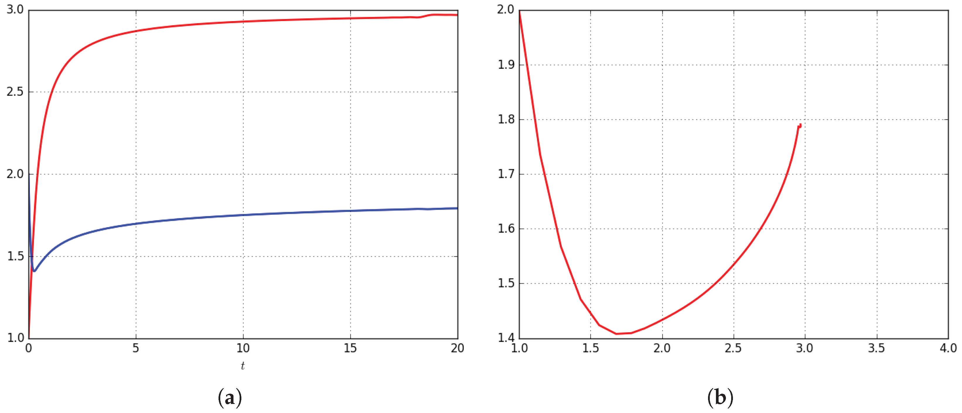
First of all, we considered the Lotka-Volterra model of fractional order, i.e., the predator-prey model with constant coefficients given in (4). We set for the prey growth rate, for the prey death rate, for the predator growth rate, for the predator death rate, and set and for the initial values of the prey and predator populations, respectively. We used the proposed collocation method to solved the problem for . The numerical solutions in the interval [0,20] are displayed in Figure 2, Figure 3, Figure 4, Figure 5 and Figure 6.
3.2. The Predator-Prey Model with Variable Coefficients
In the second set of tests we solved the predator-prey problem (1) for two sets of variable coefficients:
and
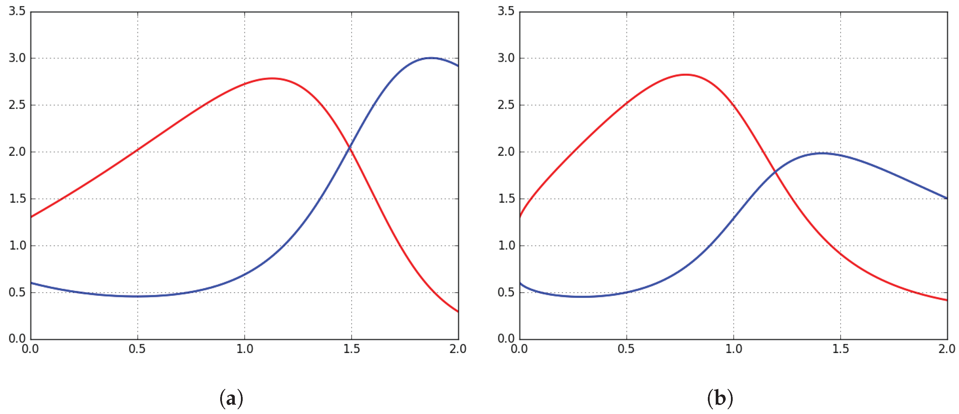
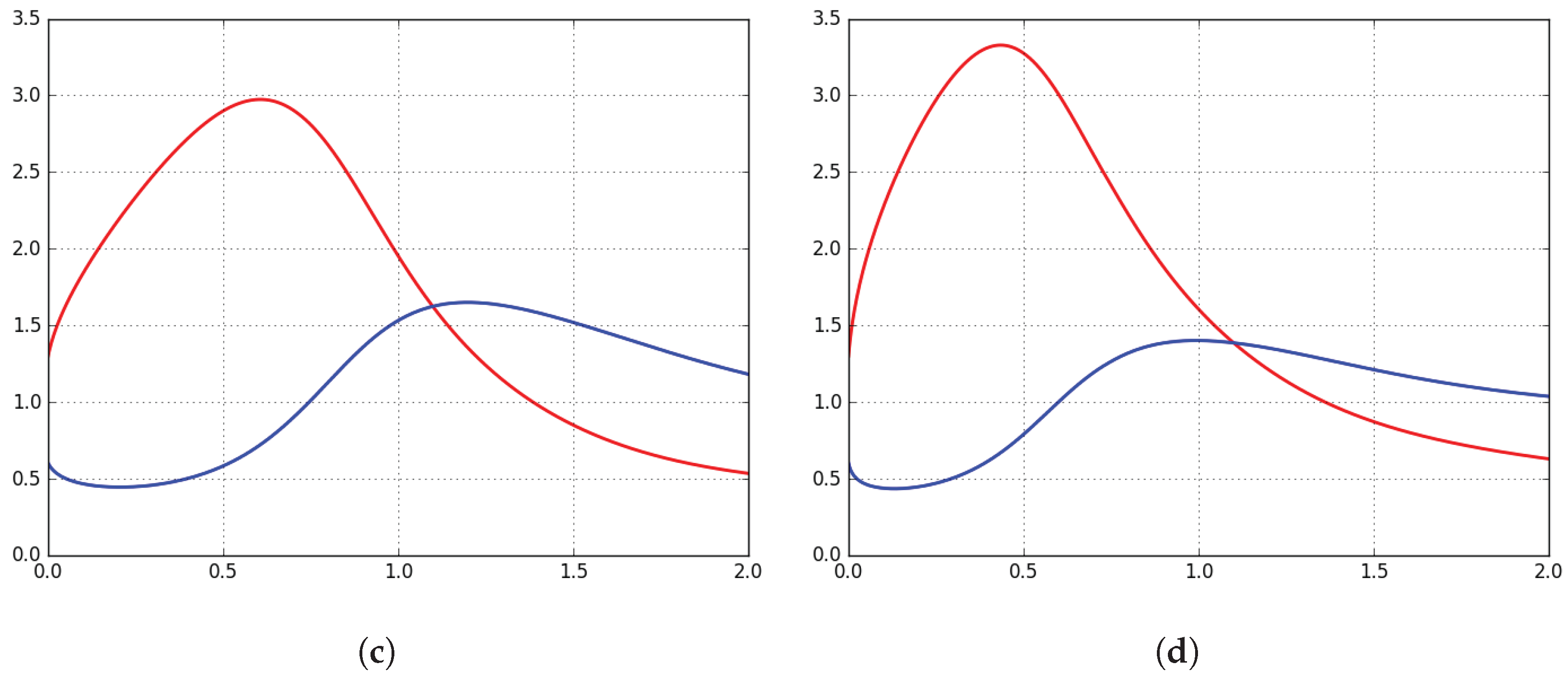
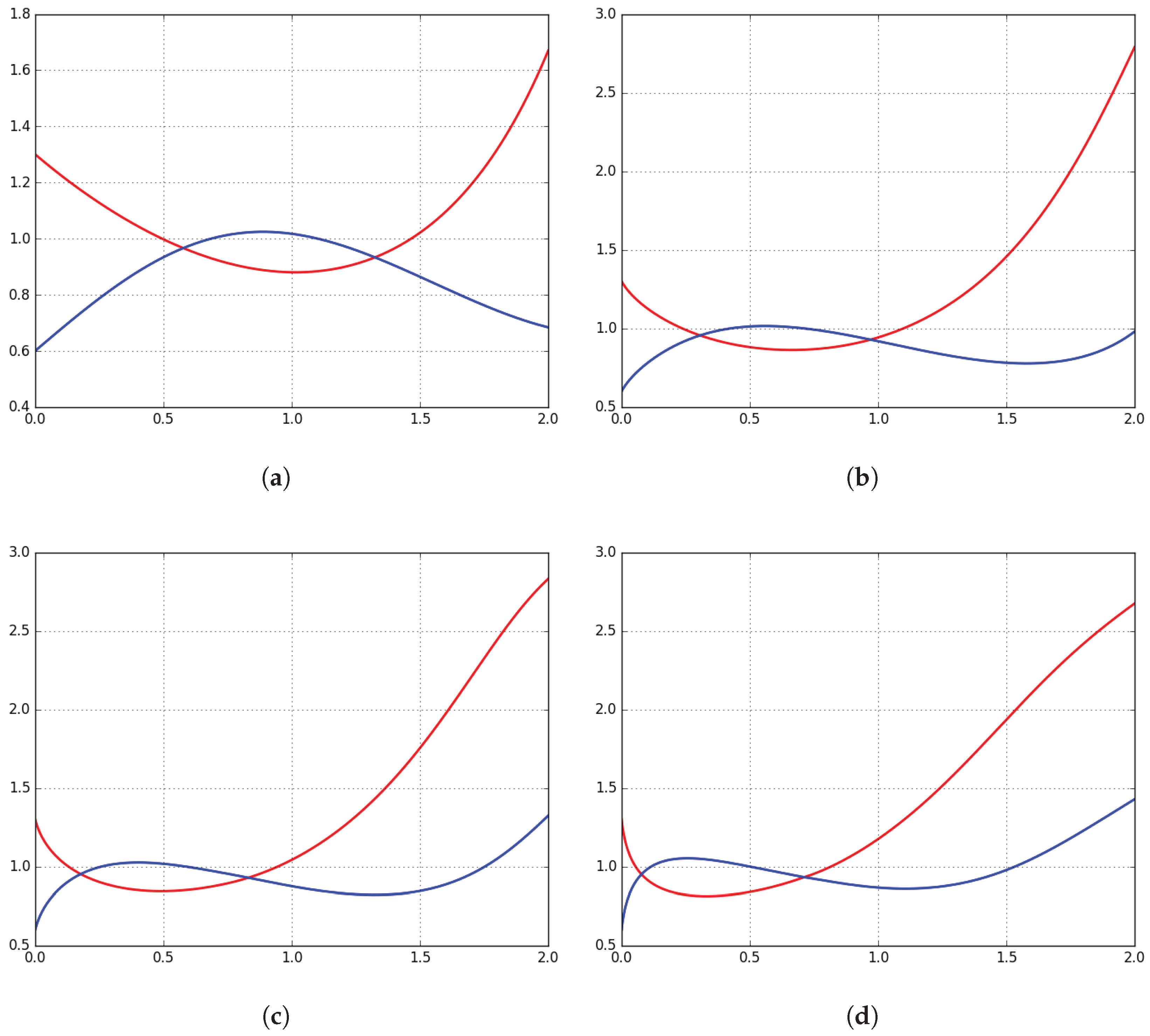
In the first case, the growth rates of both prey and predator increase with time while the death rates are constant. In the second case, the growth rates are constant while the death rates increase with time. In the numerical tests we set , and (cf. [22]). The numerical solutions in the interval [0,2] are displayed in Figure 7 and Figure 8.
4. Discussion
The numerical simulations in the previous section show that, as expected, the fractional order influences the population growth. In particular, the solution of the fractional Lotka-Volterra model is not periodic and the predator and prey populations reach the equilibrium point after an intial oscillatory behavior: the lower the derivative order is, the faster the equilibrium point is reached. As for the predator-prey model with variable coefficients, in Case since the growth rate of both predator and prey increases with time, the two populations increase for a prolonged amount of time. Before increasing, the prey population has an initial decrease while the predator population reaches a local maximum. The order of the fractional derivative influences the time after which the two populations start to increase: the lower the derivative order, the shorter the time. In Case since the predator and prey death rates increase, after an initial increase both populations decrease for long times. In addition, in this case the initial increasing is influenced by the order of the fractional derivative being shorter when the fractional derivative is lower.
Since the predator-prey model can not be solved exactly, to evaluate the performance of the proposed method we compare the numerical results in the previous section with the approximate solutions obtained by the methods proposed in [22,72]. In particular, in [72] the classical Lotka-Volterra model was solved using the the predictor-corrector method proposed in [32,33] while the predator-prey model with variable coefficients was solved in [22] by the homotopy perturbation method [21,25].
Figure 2, Figure 3 and Figure 4 show that the approximate solutions of the fractional Lotka-Volterra model produced by our collocation method are in good agreement with those ones displayed in [72] where just the values were considered. In the case of derivative of integer order, the numerical solution in Figure 2 is periodic and does not suffer from instabilities as in the case of the predictor-corrector method. In fact, the phase state diagram in Figure 2b is a closed curve while the diagram in (Figure 6 [72]) is a slightly increasing orbit. As stated by the theory in [72], when the derivative has fractional order, the numerical solution tends to the equilibrium point having coordinates (cf. Figure 3 and Figure 4). The little inaccuracy—less than 0.7—in the approximation of the y coordinate of the equilibrium point is of the same order as in [72]. Figure 5 and Figure 6 show that the error in approximating the equilibrium point increases when decreases.
For the predator-prey model with variable coefficients, the numerical solutions displayed in Figure 7, which correspond to Case , are very similar to the approximate solutions obtained in [22]. Instead, the numerical solutions for Case shown in Figure 8 are rather different from the approximate solution displayed in [22]. The reason is that just four terms of the expansion series are used to evaluate the approximations while the homotopy perturbation method requires more terms to well approximate the solution in large interval (cf. [70] where a modification of the homotopy perturbation method is used and the solution is approximated using eight terms in the series). In fact, our numerical solution and the approximate solution in [22] are comparable near the origin.
To give an idea of the accuracy of the numerical solutions displayed in Section 3, we solved the predator-prey problem for decreasing values of the distance between the knots of the partition and evaluate the infinity norm of their difference. The values of the norm, listed in Table 1, Table 2 and Table 3, show that the difference decreases when decreases reaching a value in the order of when and a value in the order of or less when is of fractional order. As a consequence, we can argue that the numerical approximations obtained by the collocation method is sufficiently accurate also in the case of derivatives of fractional order and, in particular, of small order, which are more difficult to approximate.
Then, we solved the three models for different values of . Several numerical tests not displayed here show that the numerical solution depends very little on so that the accuracy does not increase sufficiently fast when reducing the time-step.
5. Conclusions
We used a new collocation method to numerically solve some predator-prey models of fractional order. The numerical results show that the method is accurate and efficient. A theoretical proof of the convergence of the method when and go to zero follows from classical arguments in approximation theory (cf. [62]).
Some issues should be further analyzed to improve the method. First of all, the truncation of the basis functions , when restricted to the interval , produces few instabilities near the boundaries of the discretization interval; this could increase the ill-conditioning of the nonlinear system (21). A different approach should be used to generate stable bases on the interval (see, for instance, [76]). Another issue could arise from the truncation of the fractional B-spline that is necessary for numerical purposes. Finally, a different distribution of the collocation nodes could improve the accuracy of the method. These details will be analyzed in a forthcoming paper.
Conflicts of Interest
The author declares no conflict of interest.
References
- Diethelm, K. The Analysis of Fractional Differential Equations: An Application-Oriented Exposition Using Differential Operators of Caputo Type; Springer: Berlin, Germany, 2010. [Google Scholar]
- Oldham, K.; Spanier, J. The Fractional Calculus; Academic Press: Cambridge, MA, USA, 1974. [Google Scholar]
- Podlubny, I. Fractional Differential Equations; Academic Press: Cambridge, MA, USA, 1998. [Google Scholar]
- Samko, S.G.; Kilbas, A.A.; Marichev, O.I. Fractional Integrals and Derivatives; Gordon & Breach Science Publishers: Philadelphia, PA, USA, 1993. [Google Scholar]
- Hilfer, R. Applications of Fractional Calculus in Physics; World Scientific: Singapore, 2000. [Google Scholar]
- Kilbas, A.A.; Srivastava, H.M.; Trujillo, J.J. Theory and Applications of Fractional Differential Equations; Elsevier Science (North-Holland): Amsterdam, The Netherlands, 2006. [Google Scholar]
- Mainardi, F. Fractional Calculus and Waves in Linear Viscoelasticity: An Introduction to Mathematical Models; World Scientific: Singapore, 2010. [Google Scholar]
- Sabatier, J.; Agrawal, O.; Tenreiro Machado, J.A. Advances in Fractional Calculus; Springer: Berlin, Germany, 2007. [Google Scholar]
- Tarasov, V.E. Fractional Dynamics. In Nonlinear Physical Science; Springer: Berlin/Heidelberg, Germany, 2010. [Google Scholar]
- Caputo, M. Linear models of dissipation whose Q is almost frequency independent—II. Geophys. J. Int. 1967, 13, 529–539. [Google Scholar] [CrossRef]
- Atangana, A.; Baleanu, D. New fractional derivatives with nonlocal and non-singular kernel: Theory and application to heat transfer model. Therm. Sci. 2016, 20, 763–769. [Google Scholar] [CrossRef]
- Atangana, A.; Koca, I. Chaos in a simple nonlinear system with Atangana-Baleanu derivatives with fractional order. Chaos Solitons Fractals 2016, 89, 447–454. [Google Scholar] [CrossRef]
- Caputo, M.; Fabrizio, M. A new definition of fractional derivative without singular kernel. Prog. Fract. Differ. Appl. 2015, 1, 1–13. [Google Scholar]
- Caputo, M.; Fabrizio, M. Applications of new time and spatial fractional derivatives with exponential kernels. Prog. Fract. Differ. Appl. 2016, 2, 1–11. [Google Scholar] [CrossRef]
- Tateishi, A.A.; Ribeiro, H.V.; Lenzi, E.K. The role of fractional time-derivative operators on anomalous diffusion. Front. Phys. 2017, 5, 52. [Google Scholar] [CrossRef]
- Kilbas, A.A.; Trujillo, J.J. Differential equations of fractional order: Methods, results and problems. I. Appl. Anal. 2001, 78, 153–192. [Google Scholar] [CrossRef]
- Kilbas, A.A.; Trujillo, J.J. Differential equations of fractional orders: Methods, results and problems. II. Appl. Anal. 2002, 81, 435–493. [Google Scholar] [CrossRef]
- He, J.H. A tutorial review on fractal spacetime and fractional calculus. Int. J. Theor. Phys. 2014, 53, 3698–3718. [Google Scholar] [CrossRef]
- Gorenflo, R.; Kilbas, A.A.; Mainardi, F.; Rogosin, S.V. Mittag-Leffler Functions, Related Topics and Applications; Springer Monographs in Mathematics; Springer: Berlin/Heidelberg, Germany, 2014. [Google Scholar]
- Adomian, G. Solving Frontier Problems of Physics: The Decomposition Method; Springer Science & Business Media: Dordrecht, The Netherlands, 2013; Volume 60. [Google Scholar]
- He, J.H. Homotopy perturbation technique. Comput. Methods Appl. Mech. Eng. 1999, 178, 257–262. [Google Scholar] [CrossRef]
- Das, S.; Gupta, P.K. A mathematical model on fractional Lotka-Volterra equations. J. Theor. Biol. 2011, 277, 1–6. [Google Scholar] [CrossRef] [PubMed]
- Das, S.; Gupta, P.K.; Rajeev. A fractional predator-prey model and its solution. Int. J. Nonlinear Sci. Numer. Simul. 2009, 10, 873–876. [Google Scholar] [CrossRef]
- Momani, S.; Odibat, Z. Comparison between the homotopy perturbation method and the variational iteration method for linear fractional partial differential equations. Comput. Math. Appl. 2007, 54, 910–919. [Google Scholar] [CrossRef]
- Momani, S.; Odibat, Z. Homotopy perturbation method for nonlinear partial differential equations of fractional order. Phys. Lett. A 2007, 365, 345–350. [Google Scholar] [CrossRef]
- Momani, S.; Shawagfeh, N. Decomposition method for solving fractional Riccati differential equations. Appl. Math. Comput. 2006, 182, 1083–1092. [Google Scholar] [CrossRef]
- Shawagfeh, N.T. Analytical approximate solutions for nonlinear fractional differential equations. Appl. Math. Comput. 2002, 131, 517–529. [Google Scholar] [CrossRef]
- Wang, Q. Homotopy perturbation method for fractional KdV-Burgers equation. Chaos Solitons Fractals 2008, 35, 843–850. [Google Scholar] [CrossRef]
- Lubich, C. On the stability of linear multistep methods for Volterra convolution equations. IMA J. Numer. Anal. 1983, 3, 439–465. [Google Scholar] [CrossRef]
- Lubich, C. Discretized fractional calculus. SIAM J. Math. Anal. 1986, 17, 704–719. [Google Scholar] [CrossRef]
- Gorenflo, R.; Mainardi, F. Random walk models for space-fractional diffusion processes. Fract. Calc. Appl. Anal. 1998, 1, 167–191. [Google Scholar]
- Diethelm, K.; Ford, N.J.; Freed, A.D. A predictor-corrector approach for the numerical solution of fractional differential equations. Nonlinear Dyn. 2002, 29, 3–22. [Google Scholar] [CrossRef]
- Diethelm, K.; Ford, N.J.; Freed, A.D. Detailed error analysis for a fractional Adams method. Numer. Algorithms 2004, 36, 31–52. [Google Scholar] [CrossRef]
- Galeone, L.; Garrappa, R. Fractional Adams-Moulton methods. Math. Comput. Simul. 2008, 79, 1358–1367. [Google Scholar] [CrossRef]
- Baleanu, D.; Diethelm, K.; Scalas, E.; Trujillo, J.J. Fractional Calculus: Models and Numerical Methods; World Scientific: Singapore, 2016. [Google Scholar]
- Diethelm, K.; Ford, J.M.; Ford, N.J.; Weilbeer, M. Pitfalls in fast numerical solvers for fractional differential equations. J. Comput. Appl. Math. 2006, 186, 482–503. [Google Scholar] [CrossRef] [Green Version]
- Sugimoto, N. Burgers equation with a fractional derivative: Hereditary effects on nonlinear acoustic waves. J. Fluid Mech. 1991, 225, 631–653. [Google Scholar] [CrossRef]
- Doha, E.H.; Bhrawy, A.H.; Ezz-Eldien, S.S. Efficient Chebyshev spectral methods for solving multi-term fractional orders differential equations. Appl. Math. Modell. 2011, 35, 5662–5672. [Google Scholar] [CrossRef]
- Hanert, E.; Piret, C. A Chebyshev pseudo-spectral method to solve the space-time tempered fractional diffusion equation. SIAM J. Sci. Comput. 2014, 36, A1797–A1812. [Google Scholar] [CrossRef]
- Khader, M.M. On the numerical solutions for the fractional diffusion equation. Commun. Nonlinear Sci. Numer. Simul. 2011, 16, 2535–2542. [Google Scholar] [CrossRef]
- Zayernouri, M.; Karniadakis, G.E. Fractional spectral collocation method. SIAM J. Sci. Comput. 2014, 36, A40–A62. [Google Scholar] [CrossRef]
- Ervin, V.J.; Führer, T.; Heuer, N.; Karkulik, M. DPG method with optimal test functions for a fractional advection diffusion equation. J. Sci. Comput. 2017, 72, 568–585. [Google Scholar] [CrossRef]
- Li, X.; Xu, C. A space-time spectral method for the time fractional diffusion equation. SIAM J. Numer. Anal. 2009, 47, 2108–2131. [Google Scholar] [CrossRef]
- Li, X.; Xu, C. Existence and uniqueness of the weak solution of the space-time fractional diffusion equation and a spectral method approximation. Commun. Comput. Phys. 2010, 8, 1016–1051. [Google Scholar] [CrossRef]
- Wang, H.; Zhang, X. A high-accuracy preserving spectral Galerkin method for the Dirichlet boundary-value problem of variable-coefficient conservative fractional diffusion equations. J. Comput. Phys. 2015, 281, 67–81. [Google Scholar] [CrossRef]
- Zayernouri, M.; Ainsworth, M.; Karniadakis, G.E. A unified Petrov-Galerkin spectral method for fractional PDEs. Comput. Methods Appl. Mech. Eng. 2015, 283, 1545–1569. [Google Scholar] [CrossRef]
- Blank, L. Numerical treatment of differential equations of fractional order. Nonlinear World 1997, 4, 473–492. [Google Scholar]
- Pedas, A.; Tamme, E. On the convergence of spline collocation methods for solving fractional differential equations. J. Comput. Appl. Math. 2011, 235, 3502–3514. [Google Scholar] [CrossRef]
- Pedas, A.; Tamme, E. Numerical solution of nonlinear fractional differential equations by spline collocation methods. J. Comput. Appl. Math. 2014, 255, 216–230. [Google Scholar] [CrossRef]
- Ervin, V.J.; Roop, J.P. Variational solution of fractional advection dispersion equations on bounded domains in d. Numer. Methods Part. Differ. Equat. 2007, 23, 256–281. [Google Scholar] [CrossRef]
- Ford, N.J.; Xiao, J.; Yan, Y. A finite element method for time fractional partial differential equations. Fract. Calc. Appl. Anal. 2011, 14, 454–474. [Google Scholar] [CrossRef] [Green Version]
- Liu, Q.; Liu, F.; Turner, I.; Anh, V. Finite element approximation for a modified anomalous subdiffusion equation. Appl. Math. Modell. 2011, 35, 4103–4116. [Google Scholar] [CrossRef]
- Xu, Q.; Hesthaven, J.S. Discontinuous Galerkin method for fractional convection-diffusion equations. SIAM J. Numer. Anal. 2014, 52, 405–423. [Google Scholar] [CrossRef]
- Wang, H.; Yang, D.; Zhu, S. Inhomogeneous Dirichlet boundary-value problems of space-fractional diffusion equations and their finite element approximations. SIAM J. Numer. Anal. 2014, 52, 1292–1310. [Google Scholar] [CrossRef]
- Chen, Y.; Wu, Y.; Cui, Y.; Wang, Z.; Jin, D. Wavelet method for a class of fractional convection-diffusion equation with variable coefficients. J. Comput. Sci. 2010, 1, 146–149. [Google Scholar] [CrossRef]
- Li, Y. Solving a nonlinear fractional differential equation using Chebyshev wavelets. Commun. Nonlinear Sci. Numer. Simul. 2010, 15, 2284–2292. [Google Scholar] [CrossRef]
- Li, X. Numerical solution of fractional differential equations using cubic B-spline wavelet collocation method. Commun. Nonlinear Sci. Numer. Simul. 2012, 17, 3934–3946. [Google Scholar] [CrossRef]
- Li, Y.; Zhao, W. Haar wavelet operational matrix of fractional order integration and its applications in solving the fractional order differential equations. Appl. Math. Comput. 2010, 216, 2276–2285. [Google Scholar] [CrossRef]
- Rehman, M.; Khan, R.A. The Legendre wavelet method for solving fractional differential equations. Commun. Nonlinear Sci. Numer. Simul. 2011, 16, 4163–4173. [Google Scholar] [CrossRef]
- Li, C.; Chen, A. Numerical methods for fractional partial differential equations. Int. J. Comput. Math. 2017, 1–52. [Google Scholar] [CrossRef]
- Podlubny, I.; Skovranek, T.; Datsko, B. Recent advances in numerical methods for partial fractional differential equations. In Proceedings of the 2014 15th International Carpathian Control Conference (ICCC), Velke Karlovice, Czech Republic, 28–30 May 2014; pp. 454–457. [Google Scholar]
- Pezza, L.; Pitolli, F. A multiscale collocation method for fractional differential problems. Math. Comput. Simul. 2018, 147, 210–219. [Google Scholar] [CrossRef]
- Pitolli, F.; Pezza, L. A fractional spline collocation method for the fractional-order logistic equation. In Approximation Theory XV: San Antonio 2016; Springer: Berlin, Germany, 2017; pp. 307–318. [Google Scholar]
- Pezza, L.; Pitolli, F. A fractional spline collocation-Galerkin method for the time-fractional diffusion equation. 2018, in press. [Google Scholar]
- Unser, M.; Blu, T. Fractional splines and wavelets. SIAM Rev. 2000, 42, 43–67. [Google Scholar] [CrossRef]
- Lotka, A.J. Elements of Physical Biology. In Science Progress in the Twentieth Century (1919–1933); 1926, 21, 341–343. [Google Scholar]
- Volterra, V. Variazioni e fluttuazioni del numero d’individui in specie animali conviventi. Memorie della R. Accademia dei Lincei 1926, 6, 31–113. [Google Scholar]
- Murray, J.D. Mathematical Biology. I. an Introduction; Springer: Berlin/Heidelberg, Germany, 2002. [Google Scholar]
- Ahmed, E.; Elgazzar, A. On fractional order differential equations model for nonlocal epidemics. Phys. A Stat. Mech. Appl. 2007, 379, 607–614. [Google Scholar] [CrossRef]
- Kumar, S.; Kumar, A.; Odibat, Z.M. A nonlinear fractional model to describe the population dynamics of two interacting species. Math. Methods Appl. Sci. 2017, 40, 4134–4148. [Google Scholar] [CrossRef]
- Rivero, M.; Trujillo, J.J.; Vázquez, L.; Velasco, M. Fractional dynamics of populations. Appl. Math. Comput. 2011, 218, 1089–1095. [Google Scholar] [CrossRef]
- Ahmed, E.; El-Sayed, A.M.; El-Saka, H.A. Equilibrium points, stability and numerical solutions of fractional-order predator-prey and rabies models. J. Math. Anal. Appl. 2007, 325, 542–553. [Google Scholar] [CrossRef]
- Elsadany, A.A.; Matouk, A.E. Dynamical behaviors of fractional-order Lotka-Volterra predator-prey model and its discretization. J. Appl. Math. Comput. 2015, 49, 269–283. [Google Scholar] [CrossRef]
- Chen, Y.; Wei, Y.; Zhou, X.; Wang, Y. Stability for nonlinear fractional order systems: an indirect approach. Nonlinear Dyn. 2017, 89, 1–8. [Google Scholar] [CrossRef]
- Schumaker, L.L. Spline Functions: Basic Theory; Cambridge University Press: Cambridge, UK, 2007. [Google Scholar]
- Gori, L.; Pezza, L.; Pitolli, F. Recent results on wavelet bases on the interval generated by GP refinable functions. Appl. Numer. Math. 2004, 51, 549–563. [Google Scholar] [CrossRef]
Figure 1.
(a) The fractional B-splines and the polynomial B-splines for ranging from 0 to 5. The fractional derivatives of the B-splines of degree (b), (c) and (d) for . The ordinary first derivative is displayed as a dashed line while the B-spline is displayed as a dotted line.
Figure 1.
(a) The fractional B-splines and the polynomial B-splines for ranging from 0 to 5. The fractional derivatives of the B-splines of degree (b), (c) and (d) for . The ordinary first derivative is displayed as a dashed line while the B-spline is displayed as a dotted line.
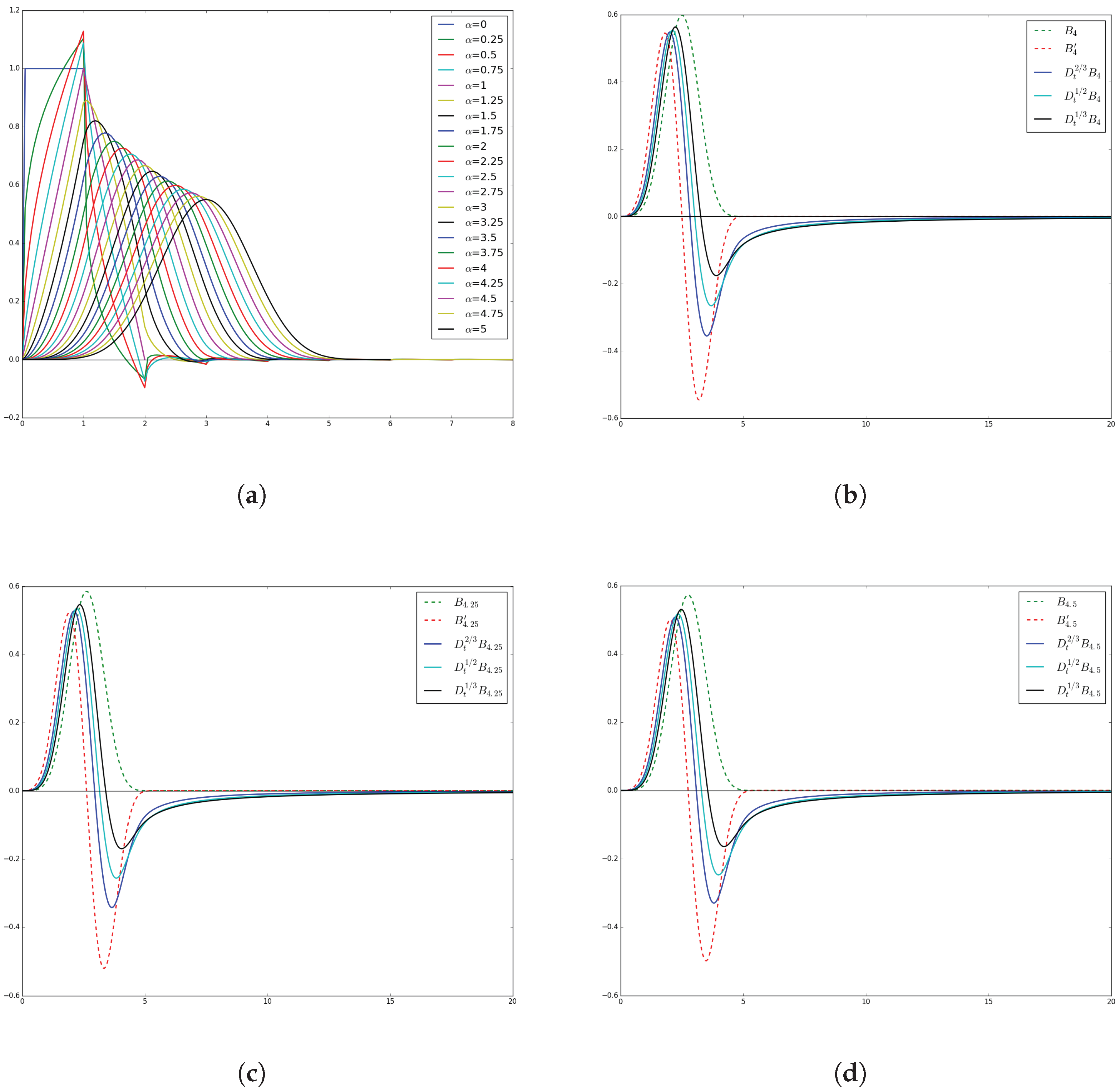
Figure 2.
(a) The numerical solution of the classical Lotka-Volterra model of integer order. The blue and red lines represent predator and prey populations, respectively; (b) The phase state diagram.
Figure 2.
(a) The numerical solution of the classical Lotka-Volterra model of integer order. The blue and red lines represent predator and prey populations, respectively; (b) The phase state diagram.
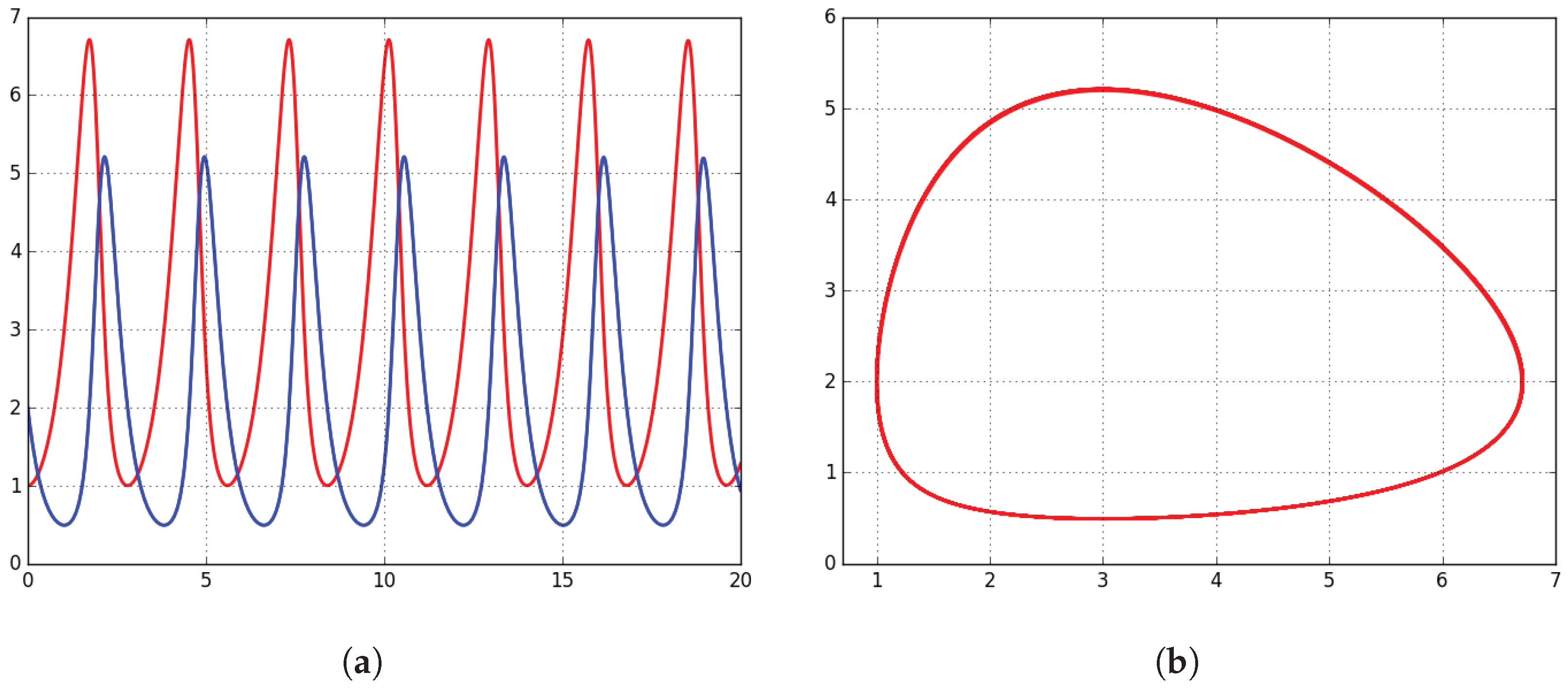
Figure 3.
(a) The numerical solution of the fractional Lotka-Volterra model for . The blue and red lines represent predator and prey populations, respectively; (b) The phase state diagram.
Figure 3.
(a) The numerical solution of the fractional Lotka-Volterra model for . The blue and red lines represent predator and prey populations, respectively; (b) The phase state diagram.
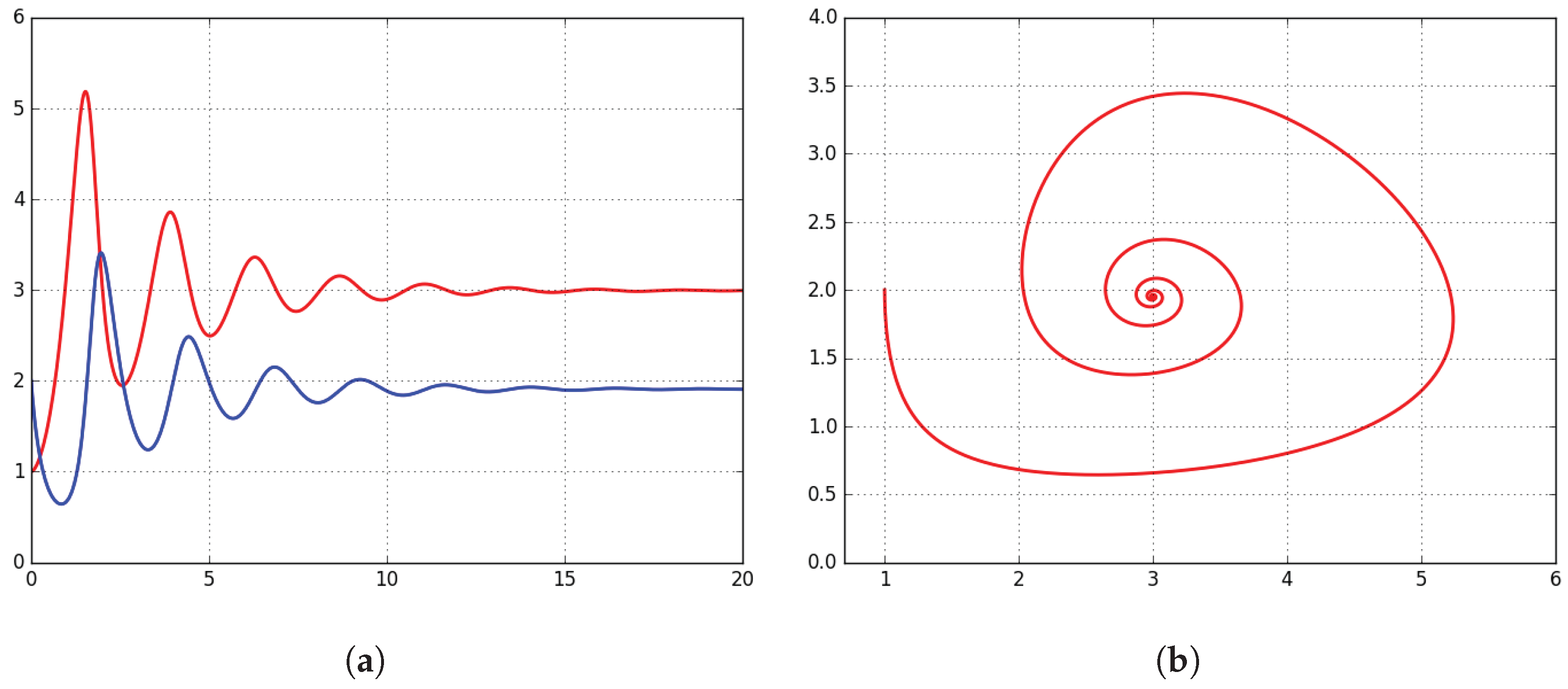
Figure 4.
(a) The numerical solution of the fractional Lotka-Volterra model for . The blue and red lines represent predator and prey populations, respectively; (b) The phase state diagram.
Figure 4.
(a) The numerical solution of the fractional Lotka-Volterra model for . The blue and red lines represent predator and prey populations, respectively; (b) The phase state diagram.
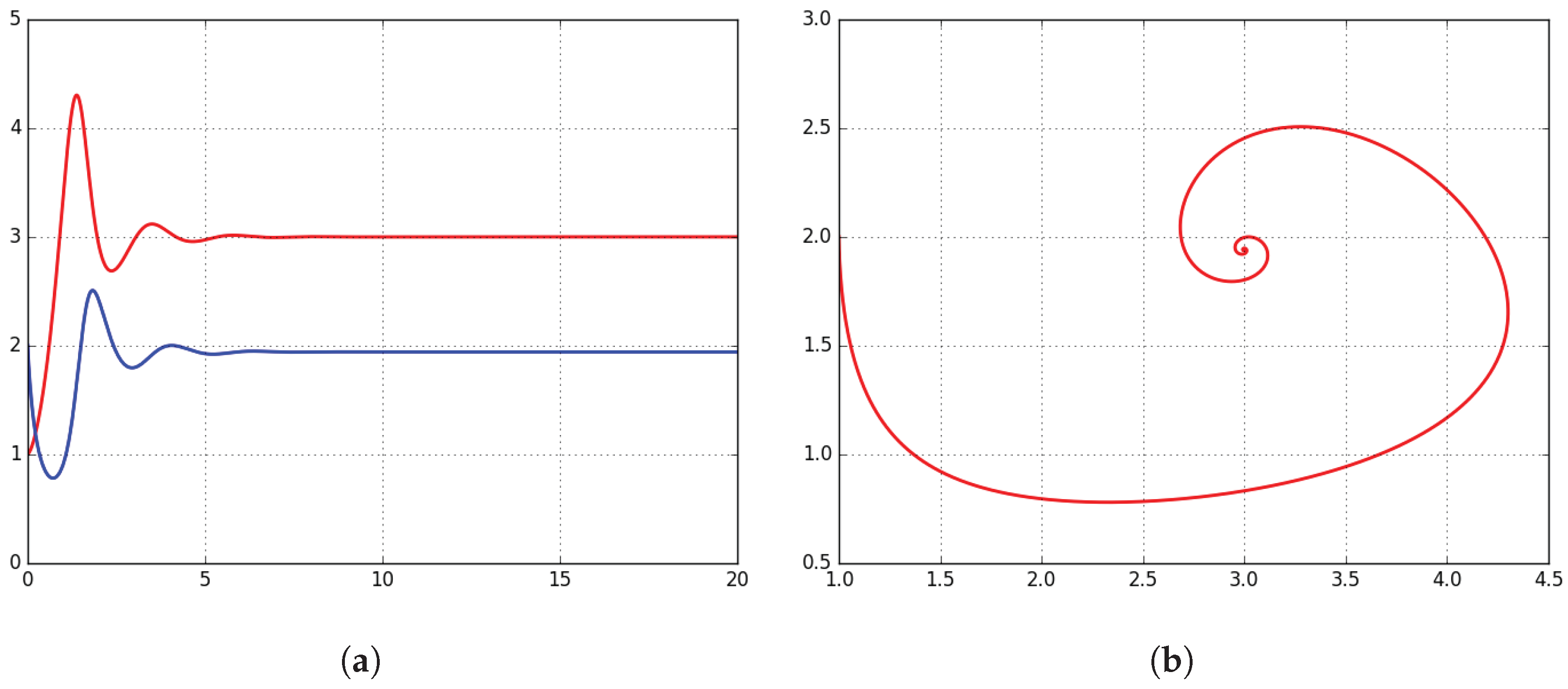
Figure 5.
(a) The numerical solution of the fractional Lotka-Volterra model for . The blue and red lines represent predator and prey populations, respectively; (b) The phase state diagram.
Figure 5.
(a) The numerical solution of the fractional Lotka-Volterra model for . The blue and red lines represent predator and prey populations, respectively; (b) The phase state diagram.
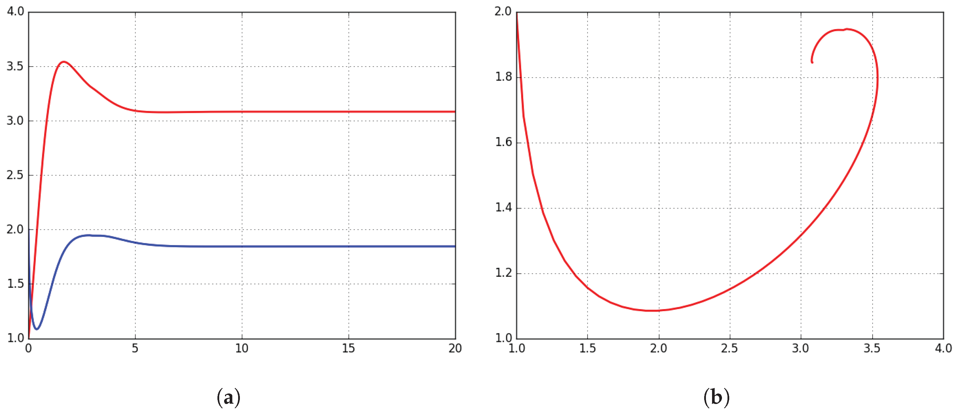
Figure 6.
(a) The numerical solution of the fractional Lotka-Volterra model for . The blue and red lines represent predator and prey populations, respectively; (b) The phase state diagram.
Figure 6.
(a) The numerical solution of the fractional Lotka-Volterra model for . The blue and red lines represent predator and prey populations, respectively; (b) The phase state diagram.

Figure 7.
The numerical solutions of the predator-prey model Case for integer order (a) and fractional order (b), (c), (d). The blue and red lines represent predator and prey populations, respectively.
Figure 7.
The numerical solutions of the predator-prey model Case for integer order (a) and fractional order (b), (c), (d). The blue and red lines represent predator and prey populations, respectively.

Figure 8.
The numerical solutions of the predator-prey model Case for integer order (a) and fractional order (b), (c), (d). The blue and red lines represent predator and prey populations, respectively.
Figure 8.
The numerical solutions of the predator-prey model Case for integer order (a) and fractional order (b), (c), (d). The blue and red lines represent predator and prey populations, respectively.

Table 1.
The Lotka-Volterra model: The infinity norm of the difference between the numerical solutions obtained using two values the distance between the partition knots, say and . Each column lists the values and for decreasing values of .
Table 1.
The Lotka-Volterra model: The infinity norm of the difference between the numerical solutions obtained using two values the distance between the partition knots, say and . Each column lists the values and for decreasing values of .
| 1 | ; | ; | ; | |
| ; | ; | ; | ||
| ; | ; | ; | ||
| ; | ; | ; | ||
| ; | ; | ; | ||
Table 2.
The predator-prey model Case : The infinity norm of the difference between the numerical solutions obtained using two values of the distance between the partition knots, say and . Each column lists the values and for decreasing values of .
Table 2.
The predator-prey model Case : The infinity norm of the difference between the numerical solutions obtained using two values of the distance between the partition knots, say and . Each column lists the values and for decreasing values of .
| 1 | ; | ; | ; | |
| ; | ; | ; | ||
| ; | ; | ; | ||
| ; | ; | ; | ||
Table 3.
The predator-prey model Case : The infinity norm of the difference between the numerical solutions obtained using two values of the distance between the partition knots, say and . Each column lists the values and for decreasing values of .
Table 3.
The predator-prey model Case : The infinity norm of the difference between the numerical solutions obtained using two values of the distance between the partition knots, say and . Each column lists the values and for decreasing values of .
| 1 | ; | ; | ; | |
| ; | ; | ; | ||
| ; | ; | ; | ||
| ; | ; | ; | ||
© 2018 by the author. Licensee MDPI, Basel, Switzerland. This article is an open access article distributed under the terms and conditions of the Creative Commons Attribution (CC BY) license (http://creativecommons.org/licenses/by/4.0/).
Share and Cite
MDPI and ACS Style
Pitolli, F. A Fractional B-spline Collocation Method for the Numerical Solution of Fractional Predator-Prey Models. Fractal Fract. 2018, 2, 13. https://doi.org/10.3390/fractalfract2010013
AMA Style
Pitolli F. A Fractional B-spline Collocation Method for the Numerical Solution of Fractional Predator-Prey Models. Fractal and Fractional. 2018; 2(1):13. https://doi.org/10.3390/fractalfract2010013
Chicago/Turabian StylePitolli, Francesca. 2018. "A Fractional B-spline Collocation Method for the Numerical Solution of Fractional Predator-Prey Models" Fractal and Fractional 2, no. 1: 13. https://doi.org/10.3390/fractalfract2010013