Novel Complex Wave Solutions of the (2+1)-Dimensional Hyperbolic Nonlinear Schrödinger Equation

1
Department of Computer Engineering, Faculty of Engineering, Ardahan University, 75000 Ardahan, Turkey
2
Mucur Vocational School, Ahi Evran University, 40500 Kırşehir, Turkey
3
Department of Mathematics, Faculty of Science, Firat University, 23100 Elazig, Turkey
*
Author to whom correspondence should be addressed.
Fractal Fract. 2020, 4(3), 41; https://doi.org/10.3390/fractalfract4030041
Submission received: 18 June 2020
/
Revised: 2 August 2020
/
Accepted: 11 August 2020
/
Published: 16 August 2020
(This article belongs to the Special Issue New Challenges Arising in Engineering Problems with Fractional and Integer Order)
Abstract
:This manuscript focuses on the application of the -expansion method to the (2+1)-dimensional hyperbolic nonlinear Schrödinger equation. With the help of projected method, the periodic and singular complex wave solutions to the considered model are derived. Various figures such as 3D and 2D surfaces with the selecting the suitable of parameter values are plotted.
1. Introduction
Most of the properties of nature and science explained by using nonlinear partial differential equations (NPDEs) are closely associated with the basic properties of applied sciences. Recently, NPDEs have been used to investigate properties of many real-world problems arising in fluid mechanics, population ecology, shallow-water wave propagation, plasma physics, solid-state physics, heat, quantum mechanics, optical fibers and biology. Moreover, their mathematical structures have also been presented to literature. Therefore, many effective methods such as -expansion method [1,2], -expansion method [3,4,5], rational sine–cosine function method [6], F-expansion method [7], Clarkson–Kruskal (CK) direct method [8], -expansion method [9], Bäcklund transformation method [10], modified exp-expansion function [11], the Painlevé analysis [12], -expansion method [13], modified Laplace decomposition method [14], Hirota bilinear method [15,16], homotopy analysis method [17], modified Kudryashov method [18], etc. [19,20,21,22,23,24,25,26,27,28,29,30,31,32,33,34,35,36,37,38,39,40,41,42,43,44,45,46,47] have been presented to the literature for observing of deeper properties of these models. In this sense, many detailed explanations of some methods with the regards of physical and mathematical properties have been presented by R. Conte and his team [48,49].
In this work, we consider the (2+1)-dimensional hyperbolic nonlinear Schrödinger equation (HNSE) [19]:
where is used to describe the complex field, and denote spatial and temporal variables, respectively. Nonlinear Schrödinger equations are mathematical models that correspond to basic physical phenomena that define the dynamics of optical strength propagation in single-mode optical fibers [43,44,45,46]. Many scientists have observed various properties of this model. Analytical properties to the Equation (1) have been obtained in [20], exact solutions Equation (1) using extended sinh–Gordon equation expansion method [21], via Adomian decomposition method [22], with the help of the first integral method [23] and many other properties such as instabilities of Schrödinger equation in [24] and also group-invariant solutions and conservation laws in [36].
In second section, we present the general properties of the -expansion method. This method is an extended version of the classic -expansion method. Specifically, when , solutions produced in -expansion method can be obtained. In third section, we apply the -expansion method to the governing model to find many new periodic and singular complex wave solutions. In fourth section, we discuss some important properties of new findings. In fifth section, we introduce a conclusion about the findings and figures.
2. General Properties of -Expansion Method
Consider the general form of NPDEs as:
and using wave transformation given as:
where Using Equation (3) into Equation (2) yields a nonlinear ODE as following:
The solution of Equation (4) may assumed in the following form according to projected method:
where are constants, is nonzero and real constant. With the balancing principle, we find the value of . Moreover, is defined as following:
and provides the following second order linear ordinary differential equation:
where and are real constants and non zero to be determined later. Putting the Equation (5) into Equation (4) and using Equation (6), then collect all terms with the same order of the , we obtain a system of algebraic equations for , and . Finally, when we solve the system to find the value of and , and inserting them into Equation (5), we can extract the periodic and singular complex wave solutions to the Equation (2).
3. Application of Projected Method
In this section, we apply the considered method to the Equation (1). Applying the following wave transformation defined as:
where are real constants with not zero. is velocity, is the slope of the connector between the two stable states of the solution, is the frequency, is the phase, is wavenumber, is the center of phase. Considering Equation (8) into Equation (1), we have follows:
From imaginary part, we get the following strain condition as:
Balancing in Equation (9), we get . Taking this into Equation (5), we get the following solution form
Substituting Equation (12) into Equation (9), we get the following system of equations:
Solving this system, we can find the following cases of the solutions to the Equation (1).
Case 1. Selecting the following coefficients
we have the following singular complex wave solution to the Equation (1):
where .
Case 2. When we consider another coefficient to the Equation (1) given as:
it gives another singular complex wave solution to the governing model as:
in which .
Case 3. Choosing as:
we extract the following periodic complex wave solution to the Equation (1):
where , with strain condition.
Case 4. If it is taken as following form:
produces following new complex traveling wave solution given as
where , with strain condition.
4. Results and Discussions
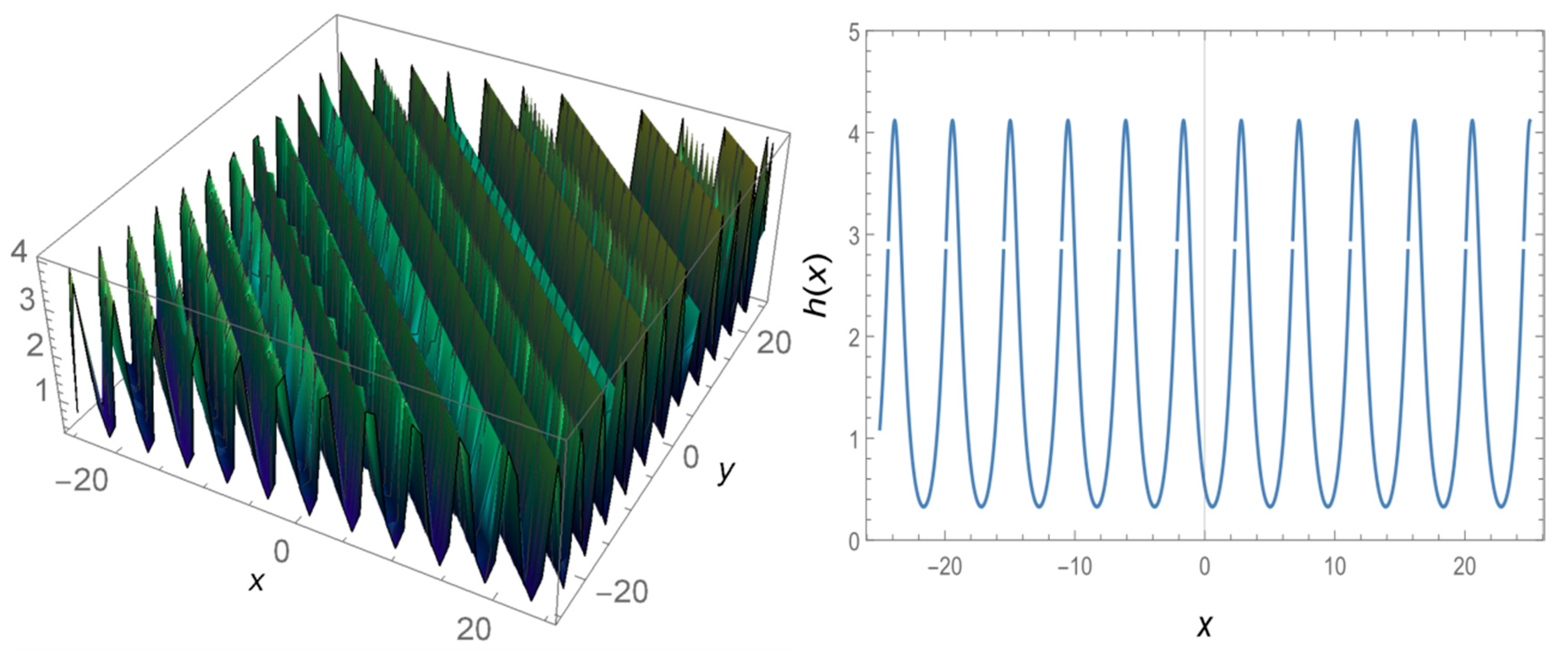
First, it may be observed that Figure 1 and Figure 2 are singular complex wave solutions to the governing model, Figure 3 and Figure 4 are periodic complex wave solutions for the Equation (1).Unlike many analytical methods, we offer different solutions from the -expansion method [25,26,27,28] which produces hyperbolic type traveling wave solution. What is interesting here is the idea that at the beginning, if , the solutions produced by the -expansion method are obtained. However, if is taken in Equation (20), is undefined. Therefore, we offered different solutions from the solution produced by the classic -expansion method. Such solutions include singular points. Solutions containing single points are important for the shock wave structure. Moreover, the solutions that provide the equation due to the structure of the Schrödinger equation are of the complex wave solution. These solutions are in hyperbolic form and are different from the solutions produced in other analytical solutions. Appropriate values are given so that the structure of the functions created by the parameters is not disrupted. The special values given to these constants have rendered to draw the shape of the wave at any given moment.
5. Conclusions
In this article, entirely new singular and periodic wave solutions to the governing model were successfully extracted via projected method. Strain conditions are also reported in this paper for validating the results. It may be also observed that these results satisfied the governing models. Figures of these solutions were plotted in 3D and 2D with the help of computational programs.
Comparing these results with the results obtained exp function solutions in [19], it may be seen that these results are entirely different solutions to the governing model. In this sense, these solutions may be also used to explain the nonlinear wave properties in defined intervals. Although it is quite difficult to obtain the solutions of NPDEs, the constructions of these solutions are facilitated with the help of some developed and modified methods. It can be also used that this method can be recommended in investigations of many other mathematical models with high nonlinearity. Considering these figures drawn in this paper and using symbolic calculation, the -expansion method was to be an effective, powerful and reliable mathematical tool for governing models.
Author Contributions
Conceptualization, H.D.; methodology, E.I.; formal analysis, and writing—review and editing, H.B. All authors have read and agreed to the published version of the manuscript.
Funding
This research received no external funding.
Acknowledgments
Authors extend their thanks to the Editors and anonymous reviewers.
Conflicts of Interest
The authors declare no conflict of interest.
References
- Ismael, H.F.; Bulut, H.; Baskonus, H.M. Optical soliton solutions to the Fokas–Lenells equation via sine-Gordon expansion method and (m + (G′/G))-expansion method. Pramana 2020, 94, 35. [Google Scholar] [CrossRef]
- Gao, W.; Ismael, H.F.; Husien, A.M.; Bulut, H.; Baskonus, H.M. Optical soliton solutions of the cubic-quartic nonlinear Schrödinger and resonant nonlinear Schrödinger equation with the parabolic law. Appl. Sci. 2020, 10, 219. [Google Scholar] [CrossRef] [Green Version]
- Yokus, A.; Durur, H.; Ahmad, H. Hyperbolic Type solutions for the couple Boiti-Leon-Pempinelli system. Facta Univ. Ser. Math. Inform. 2020, 35, 523–531. [Google Scholar]
- Ali, K.K.; Dutta, H.; Yilmazer, R.; Noeiaghdam, S. On the new wave behaviors of the Gilson-Pickering equation. Front. Phys. 2020, 8, 54. [Google Scholar] [CrossRef]
- Durur, H.; Yokuş, A. Analytical solutions of Kolmogorov–Petrovskii–Piskunov equation. J. Balikesir Univ. Inst. Sci. Technol. 2020, 22, 628–636. [Google Scholar]
- Darvishi, M.T.; Najafi, M.; Wazwaz, A.M. Construction of exact solutions in amagneto-electro-elastic circular rod. Waves Random Complex Media 2020, 30, 340–353. [Google Scholar] [CrossRef]
- Gao, W.; Silambarasan, R.; Baskonus, H.M.; Anand, R.V.; Rezazadeh, H. Periodic waves of the nondissipative double dispersive micro strain wave in the micro structured solids. Phys. A Stat. Mech. Appl. 2020, 545, 123772. [Google Scholar] [CrossRef]
- Su-Ping, Q.; Li-Xin, T. Modification of the Clarkson–Kruskal Direct method for a coupled system. Chin. Phys. Lett. 2007, 24, 2720. [Google Scholar] [CrossRef]
- Durur, H. Different types analytic solutions of the (1+1)-dimensional resonant nonlinear Schrödinger’s equation using (G′/G)-expansion method. Mod. Phys. Lett. B 2020, 34, 2050036. [Google Scholar] [CrossRef]
- Rezazadeh, H.; Kumar, D.; Neirameh, A.; Eslami, M.; Mirzazadeh, M. Applications of three methods for obtaining optical soliton solutions for the Lakshmanan–Porsezian–Daniel model with Kerr law nonlinearity. Pramana 2020, 94, 39. [Google Scholar] [CrossRef]
- Baskonus, H.M.; Bulut, H.; Atangana, A. On the complex and hyperbolic structures of the longitudinal wave equation in a magneto-electro-elastic circular rod. Smart Mater. Struct. 2016, 25, 035022. [Google Scholar] [CrossRef]
- Liu, H.; Bai, C.L.; Xin, X. Painlevé analysis, group classification and exact solutions to the nonlinear wave equations. Eur. Phys. J. B 2020, 93, 26. [Google Scholar] [CrossRef]
- Yokus, A.; Durur, H.; Ahmad, H.; Yao, S.W. Construction of different types analytic solutions for the Zhiber-Shabate quation. Mathematics 2020, 8, 908. [Google Scholar] [CrossRef]
- Yavuz, M.; Sulaiman, T.A.; Usta, F.; Bulut, H. Analysis and numerical computations of the fractional regularized long-wave equation with damping term. Math. Methods Appl. Sci. 2020. [Google Scholar] [CrossRef]
- Guan, X.; Liu, W.; Zhou, Q.; Biswas, A. Some lump solutions for a generalized (3+1)-dimensional Kadomtsev–Petviashvili equation. Appl. Math. Comput. 2020, 366, 124757. [Google Scholar] [CrossRef]
- El-Labany, S.K.; El-Taibany, W.F.; Behery, E.E.; Fouda, S.M. Collision of dustion acoustic multi solitons in a non-extensive plasma using Hirota bilinear method. Phys. Plasmas 2018, 25, 013701. [Google Scholar] [CrossRef]
- Sharma, B.; Kumar, S.; Cattani, C.; Baleanu, D. Nonlinear dynamics of Cattaneo–Christov heat flux model for third-grade power-law fluid. J. Comput. Nonlinear Dyn. 2020, 15, 011009. [Google Scholar] [CrossRef]
- Srivastava, H.M.; Baleanu, D.; Machado, J.A.T.; Osman, M.S.; Rezazadeh, H.; Arshed, S.; Günerhan, H. Traveling wave solutions to nonlinear directional couplers by modified Kudryashov method. Phys. Scr. 2020. [Google Scholar] [CrossRef]
- Ali, K.K.; Wazwaz, A.M.; Mehanna, M.S.; Osman, M.S. On short-range pulse propagation described by (2+1)-dimensional Schrödinger’s hyperbolic equation in nonlinear optical. Phys. Scr. 2020, 95, 075203. [Google Scholar] [CrossRef]
- Zayed, E.M.E.; Al-Nowehy, A.G. Exact solutions and optical soliton solutions for the (2 + 1)-dimensional hyperbolic nonlinear Schrödinger equation. Optik 2016, 127, 4970–4983. [Google Scholar] [CrossRef]
- Seadawy, A.R.; Kumar, D.; Chakrabarty, A.K. Dispersive optical soliton solutions for the hyperbolic and cubic-quintic nonlinear Schrödinger equations via the extended sinh-Gordon equation expansion method. Eur. Phys. J. Plus 2018, 133, 182. [Google Scholar] [CrossRef]
- Ahmed, I.; Chunlai, M.; Zheng, P. Exact solution of the (2+1)-dimensional hyperbolic nonlinear Schrödinger equation byAdomian decomposition method. Malaya J. Mat. 2014, 2, 160–164. [Google Scholar]
- El-Ganaini, S.I.A. The first integral method to the nonlinear Schrodinger equations in higher dimensions. Abst. Appl. Anal. 2013, 2013, 1–10. [Google Scholar] [CrossRef] [Green Version]
- Pelinovsky, D.E.; Rouvinskaya, E.A.; Kurkina, O.E.E.; Deconinck, B. Short-wave transverse instabilities of line solitons of the two-dimensional hyperbolic nonlinear Schrödinger equation. Theor. Math. Phys. 2014, 179, 452–461. [Google Scholar] [CrossRef] [Green Version]
- Yokuş, A.; Durur, H. Complex hyperbolic traveling wave solutions of Kuramoto-Sivashinsky equation using (1/G′)expansion method for nonlinear dynamic theory. J. Balikesir Univ. Inst. Sci. Technol. 2019, 21, 590–599. [Google Scholar]
- Durur, H.; Yokuş, A. Hyperbolic traveling wave solutions for Sawada–Kotera equation using (1/G′)-expansion method. Afyon Kocatepe Univ. J. Sci. Eng. Sci. 2019, 19, 615–619. [Google Scholar]
- Yokuş, A. Comparison of Caputo and conformable derivatives for time-fractional Korteweg–deVries equation via the finite difference method. Int. J. Mod. Phys. B 2018, 32, 1850365. [Google Scholar] [CrossRef]
- Yavuz, M.; Yokus, A. Analytical and numerical approaches to nerve impulse model of fractional-order. Numer. Methods Part. Differ. Equ. 2020. [Google Scholar] [CrossRef]
- Goufo, E.F.D.; Tenkam, H.M.; Khumalo, M. A behavioral analysis of KdVB equation under the law of Mittag–Leffler function. Chaos Solitons Fractals 2019, 125, 139–145. [Google Scholar] [CrossRef]
- Khan, Z.H.; Hussain, S.T.; Hammouch, Z. Flow and heat transfer analysis of water and ethyleneglycol based Cunano particles between two parallel disks with suction/injection effects. J. Mol. Liq. 2016, 221, 298–304. [Google Scholar]
- Guedda, M.; Hammouch, Z. On similarity and pseudo-similarity solutions of Falkner–Skan boundary layers. Fluid Dyn. Res. 2006, 38, 211–223. [Google Scholar] [CrossRef]
- Goufo, E.F.D.; Atangana, A. Dynamics of traveling waves of variable order hyperbolic Liouville equation: Regulation and control. Discret. Contin. Dyn. Syst. S 2019, 13, 645–662. [Google Scholar] [CrossRef] [Green Version]
- Seadawy, A.R. Stability analysis solutions for nonlinear three-dimensional modified Korteweg–de Vries–Zakharov–Kuznetsov equation in a magnetized electron–positron plasma. Phys. A Stat. Mech. Appl. 2016, 455, 44–51. [Google Scholar] [CrossRef]
- Arshad, M.; Seadawy, A.; Lu, D.; Wang, J. Travelling wave solutions of generalized coupled Zakharov–Kuznetsov and dispersive long wave equations. Results Phys. 2016, 6, 1136–1145. [Google Scholar] [CrossRef] [Green Version]
- Lu, D.; Seadawy, A.R.; Arshad, M.; Wang, J. New solitary wave solutions of (3+1)-dimensional nonlinear extended Zakharov-Kuznetsov and modified KdV-Zakharov-Kuznetsov equations and their applications. Results Phys. 2017, 7, 899–909. [Google Scholar] [CrossRef]
- Özkan, Y.S.; Yaşar, E.; Seadawy, A.R. A third-order nonlinear Schrödinger equation: The exact solutions, group-invariant solutions and conservation laws. J. Taibah Univ. Sci. 2020, 14, 585–597. [Google Scholar] [CrossRef]
- Ahmad, H.; Seadawy, A.R.; Khan, T.A.; Thounthong, P. Analytic approximate solutions for some nonlinear Parabolic dynamical wave equations. J. Taibah Univ. Sci. 2020, 14, 346–358. [Google Scholar] [CrossRef] [Green Version]
- Arnous, A.H.; Seadawy, A.R.; Alqahtani, R.T.; Biswas, A. Optical solitons with complex Ginzburg–Landau equation by modified simple equation method. Optik 2017, 144, 475–480. [Google Scholar] [CrossRef]
- Seadawy, A.R.; Jun, W. Mathematical methods and solitary wave solutions of three-dimensional Zakharov-Kuznetsov-Burgers equation in dusty plasma and its applications. Results Phys. 2017, 7, 4269–4277. [Google Scholar]
- Durur, H.; Tasbozan, O.; Kurt, A. New analytical solutions of conformable time fractional bad and good modified Boussinesq equations. Appl. Math. Nonlinear Sci. 2020, 5, 447–454. [Google Scholar] [CrossRef]
- Durur, H.; Kurt, A.; Tasbozan, O. New travelling wave solutions for KdV6 equation using sub equation method. Appl. Math. Nonlinear Sci. 2020, 5, 455–460. [Google Scholar] [CrossRef]
- Kaya, D.; Yokuş, A.; Demiroğlu, U. Comparison of exact and numerical solutions for the Sharma–Tasso–Olver equation. In Numerical Solutions of Realistic Nonlinear Phenomena; Springer: Cham, Switzerland, 2020; pp. 53–65. [Google Scholar]
- Apeanti, W.O.; Seadawy, A.R.; Lu, D. Complex optical solutions and modulation instability of hyperbolic Schrödinger dynamical equation. Results Phys. 2019, 12, 2091–2097. [Google Scholar] [CrossRef]
- Arshad, M.; Seadawy, A.R.; Lu, D. Bright–dark solitary wave solutions of generalized higher-order nonlinear Schrödinger equation and its applications in optics. J. Electromagn. Waves Appl. 2017, 31, 1711–1721. [Google Scholar] [CrossRef]
- Arshad, M.; Seadawy, A.R.; Lu, D. Exact bright–dark solitary wave solutions of the higher-order cubic–quintic nonlinear Schrödinger equation and its stability. Optik 2017, 138, 40–49. [Google Scholar] [CrossRef]
- Arshad, M.; Seadawy, A.R.; Lu, D.; Jun, W. Modulation instability analysis of modify unstable nonlinear schrodinger dynamical equation and its optical soliton solutions. Results Phys. 2017, 7, 4153–4161. [Google Scholar] [CrossRef]
- Baskonus, H.M.; Cattani, C.; Ciancio, A. Periodic, complex and kink-type solitons for the nonlinear model in microtubules. J. Appl. Sci. 2019, 21, 34–45. [Google Scholar]
- Conte, R.; Musette, M. Elliptic general analytic solutions. Stud. Appl. Math. 2009, 123, 63–81. [Google Scholar] [CrossRef]
- Conte, R.; Ng, T.W. Meromorphic solutions of a third order nonlinear differential equation. J. Math. Phys. 2010, 51, 033518. [Google Scholar] [CrossRef] [Green Version]
Figure 1.
Three-dimensional and 2D graphs of Equation (15) for values and for 2D.
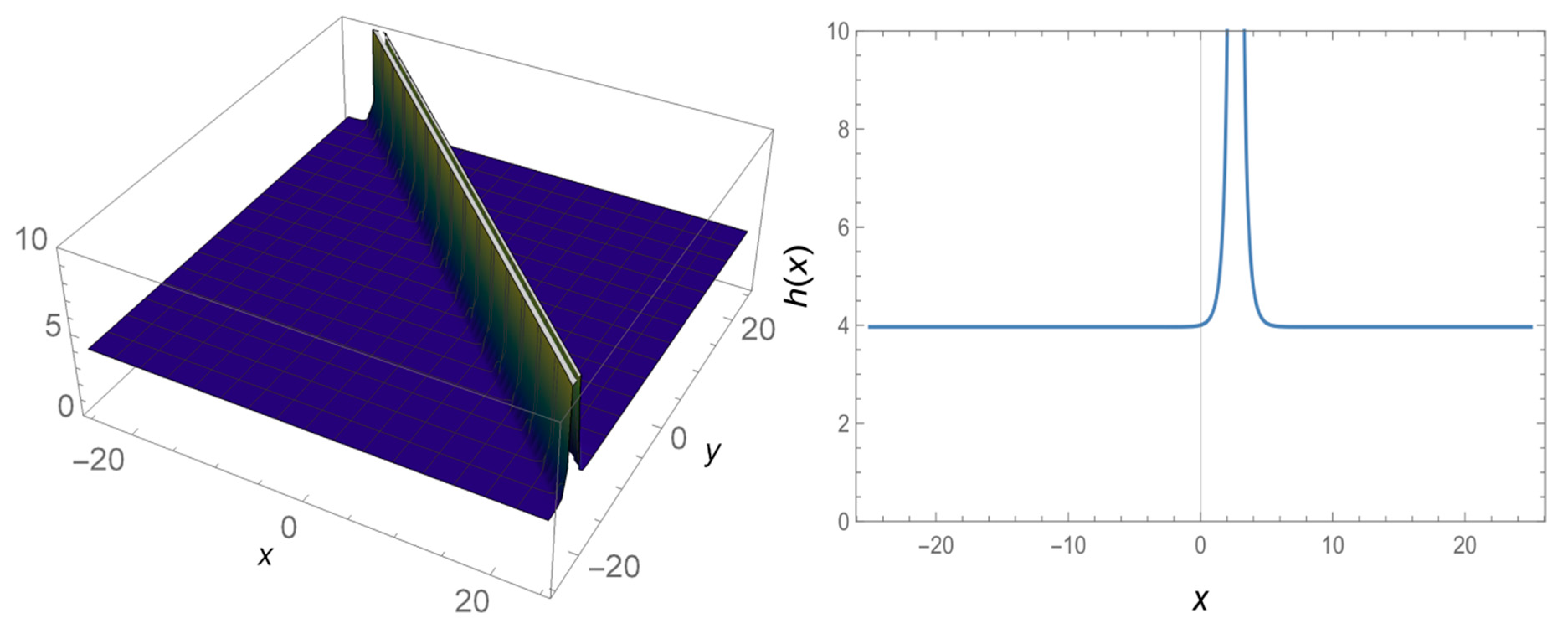
Figure 2.
Three-dimensional and 2D graphs for values of Equation (17) and for 2D.
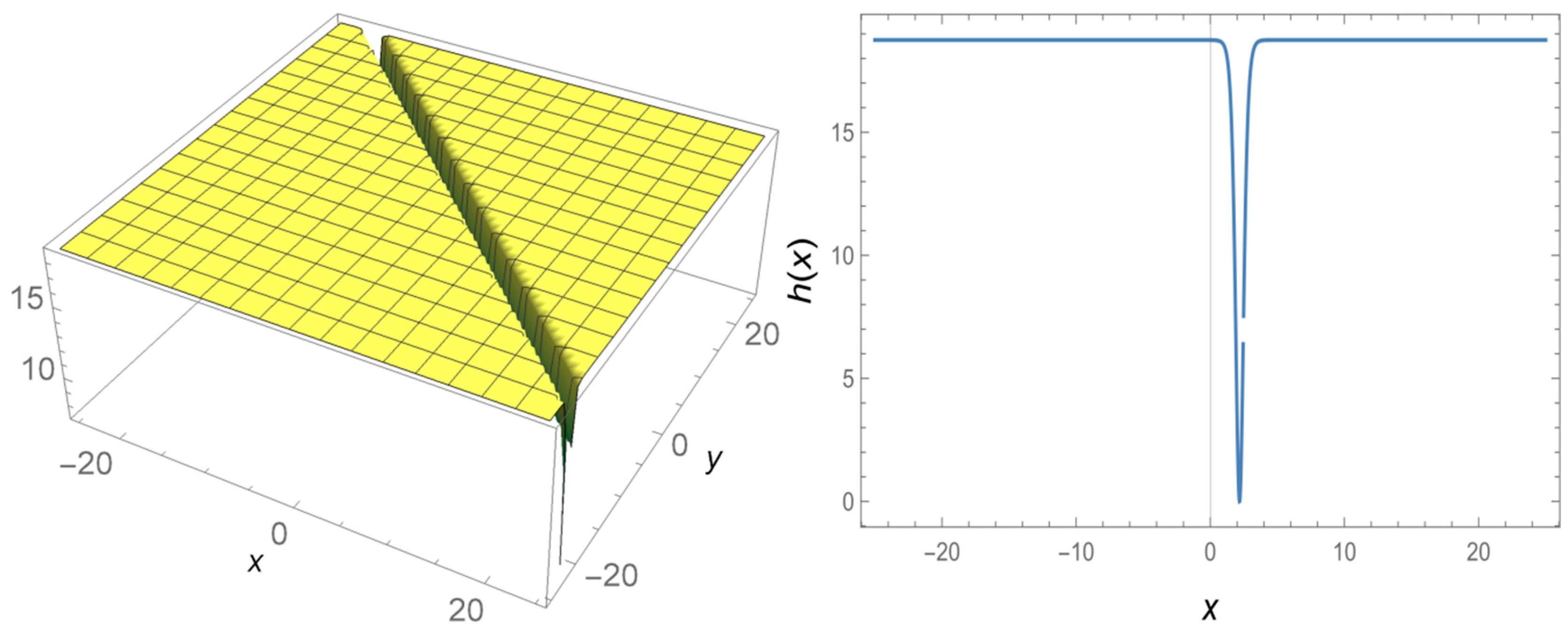
Figure 3.
Three-dimensional and 2D graphs for values of Equation (19) and for 2D.
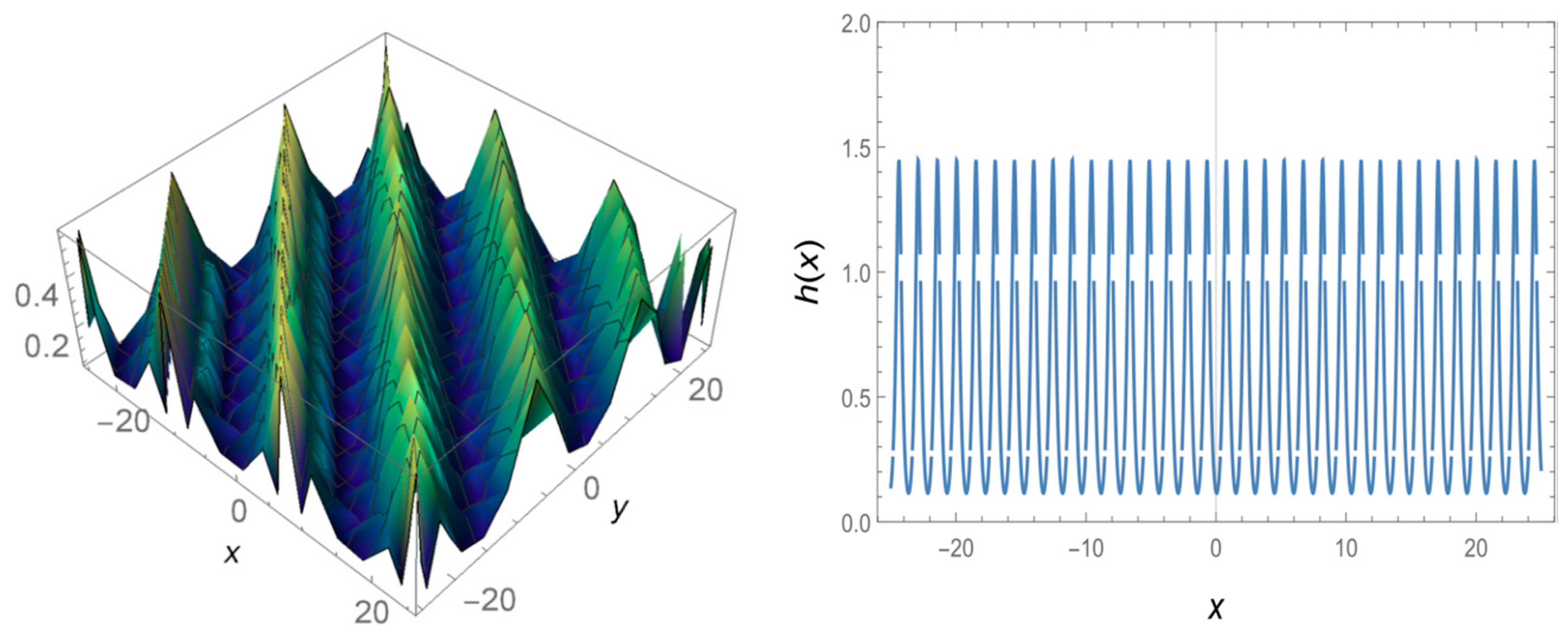
Figure 4.
Three-dimensional and 2D graphs for values of Equation (21) and for 2D.
© 2020 by the authors. Licensee MDPI, Basel, Switzerland. This article is an open access article distributed under the terms and conditions of the Creative Commons Attribution (CC BY) license (http://creativecommons.org/licenses/by/4.0/).
Share and Cite
MDPI and ACS Style
Durur, H.; Ilhan, E.; Bulut, H. Novel Complex Wave Solutions of the (2+1)-Dimensional Hyperbolic Nonlinear Schrödinger Equation. Fractal Fract. 2020, 4, 41. https://doi.org/10.3390/fractalfract4030041
AMA Style
Durur H, Ilhan E, Bulut H. Novel Complex Wave Solutions of the (2+1)-Dimensional Hyperbolic Nonlinear Schrödinger Equation. Fractal and Fractional. 2020; 4(3):41. https://doi.org/10.3390/fractalfract4030041
Chicago/Turabian StyleDurur, Hulya, Esin Ilhan, and Hasan Bulut. 2020. "Novel Complex Wave Solutions of the (2+1)-Dimensional Hyperbolic Nonlinear Schrödinger Equation" Fractal and Fractional 4, no. 3: 41. https://doi.org/10.3390/fractalfract4030041