
Finite Element Formulation of Fractional Constitutive Laws Using the Reformulated Infinite State Representation


Institute for Nonlinear Mechanics, University of Stuttgart, Pfaffenwaldring 9, 70569 Stuttgart, Germany
*
Author to whom correspondence should be addressed.
Fractal Fract. 2021, 5(3), 132; https://doi.org/10.3390/fractalfract5030132
Submission received: 19 August 2021
/
Revised: 10 September 2021
/
Accepted: 18 September 2021
/
Published: 21 September 2021
(This article belongs to the Special Issue Theory and Applications of 3D Fractional Models)
Abstract
:In this paper, we introduce a formulation of fractional constitutive equations for finite element analysis using the reformulated infinite state representation of fractional derivatives. Thereby, the fractional constitutive law is approximated by a high-dimensional set of ordinary differential and algebraic equations describing the relation of internal and external system states. The method is deduced for a three-dimensional linear viscoelastic continuum, for which the hydrostatic and deviatoric stress-strain relations are represented by a fractional Zener model. One- and two-dimensional finite elements are considered as benchmark problems with known closed form solutions in order to evaluate the performance of the scheme.
1. Introduction
The mechanical behavior of viscoelastic materials is characterized by a combined viscous and elastic material response to external loads and displacements depending on time or frequency. It is often described by complex rheological models consisting of spring-dashpot networks, which usually lead to a large number of parameters and poor extrapolation properties over several decades in time or frequency. It has been shown, though, that additional fractional-order elements, so called springpots, may lead to improved approximations, even with few parameters [1,2]. These elements are related to integrals and derivatives of non-integer order, treated within the theory of fractional calculus [3,4,5,6].
Fractional derivatives and integrals arise in viscoelasticity, when their integral kernels are used to model long-term creep and relaxation processes in the time domain. Early contributions identify a power-law behavior of viscoelastic media, see [7,8,9,10,11]. Later, this empirical observation has been connected directly to the theory of fractional calculus, see [1,12,13] and the physical consistency of fractional viscoelastic models has been discussed in [14,15]. In most applications of fractional viscoelasticity, the mechanical behavior of rubber and polymers is investigated, see e.g., [2]. Recently, fractional viscoelastic models have been used to model asphalt and concrete creep, see [16,17,18], respectively.
A key problem of fractional calculus in applications is the efficient numerical solution of fractional-order differential equations. Unfortunately, the non-locality of fractional operators usually leads to computationally expensive implementations. One possible way to overcome these difficulties is the approximation of fractional-order differential equations by high-dimensional ordinary differential equations. This approximation is based on the diffusive or infinite state representation of fractional derivatives as introduced in [19,20] and elaborated in [21,22,23,24]. The associated numerical schemes (in the following called infinite state schemes) do not require to process the entire solution history in every time step, which leads to reduced computational costs and memory requirements, whereas the accuracy depends on the chosen quadrature and order of differentiation [25,26,27,28,29].
In order to simulate the mechanical behavior of arbitrary viscoelastic structures described by fractional constitutive laws, an associated finite element formulation is required, which has to be combined with a suitable solver for fractional-order differential equations. A first formulation for linear fractional viscoelastic systems is given in [30] by using the Laplace domain. This approach has been generalized to the time domain in [31,32]. Hereto, the equations of motion are transformed to order and solved in terms of a fractional-order state space vector. The authors in [33] derive the three-dimensional generalization of a fractional viscoelastic constitutive law for the isotropic case and introduce a finite element approach solving fractional-order equations of order 2 using the Grünwald-Letnikov scheme. The formulation is generalized for the anisotropic case in [34]. Both methods use an internal variable approach, given in general form in [35]. Another formulation, see [36], which also uses the Grünwald-Letnikov scheme, incorporates the constitutive law in a slightly different way. The method is adapted and improved in [2]. All authors mentioned so far consider the geometrically linear case. Formulations in the context of large deformations are given in [37] and, recently in [38,39]. Both of the latter contributions use an infinite state scheme similar as in [40] for the time integration. An additional accuracy optimization is included in [39].
A novel improved infinite state scheme was presented in [41], but is not yet accessible for a finite element formulation of fractional constitutive laws. It is the aim of this paper to fill that gap and combine the scheme in [41] with the finite element method (FEM). The method is based on the reformulated infinite state representation, which leads to a non-singular integration kernel that asymptotically decays to zero and hence results in small errors in an associated quadrature, called reformulated infinite state scheme (RISS). The finite element formulation is fully derived for an isotropic three-dimensional continuum described by a fractional Zener model (distinguishing between hydrostatic and deviatoric stress and strain components), being a simple but archetype fractional rheological model. The method is tested on a one- and a two-dimensional example with closed form exact solutions, allowing for a proper error analysis. Moreover, the characteristic structure of the reformulated infinite state representation is interpreted in terms of viscoelastic quantities of a springpot.
The necessary theoretical preliminaries of fractional calculus are given in Section 2, including the (reformulated) infinite state representation (Section 2.2 and Section 2.3) and the scheme RISS (Section 2.4). The formulation of fractional viscoelasticity is provided in Section 3. Particularly, in Section 3.1, the terms and quantities of classical linear viscoelasticity are introduced and connected in Section 3.2 to the fractional-order case, especially the springpot and the fractional Zener model. The main results regarding FEM can be found in Section 4. It contains a three-dimensional formulation of the fractional Zener model (Section 4.1) and its implementation in the finite element method (Section 4.2). The numerical examples are studied in Section 4.3. All results are discussed in Section 5.
2. Fractional Calculus and the Reformulated Infinite State Representation
2.1. Definitions and Properties
The following concepts and properties are well-known results from fractional calculus, see e.g., [3,4,5,6]. Let and be an integrable function. The Liouville-Weyl fractional integral of x of order is introduced as [42]
where represents the Euler Gamma function
It can easily be checked that (1) simplifies to a plain primitive of x at the limit . To examine the limit for , consider the following. If, additionally, the function x is absolutely continuous (in the sense of [6] (Chapter 2, Definition 6.1)) and x and vanish in an appropriate manner in the negative time limit, we obtain by partial integration of (1)
The representation (3) shows that (1) is a plain identity for . Both limiting cases together provide the intuition that the fractional integral for is something in between the identity and the first-order primitive.
Furthermore, the Liouville-Weyl fractional derivative of Caputo type of order of an absolutely continuous function x is given as [42]
which is (one possible definition for) a left inverse of the operator , i.e.,
see [6] (Chapter 2, § 6.2). Similar to the fractional integral, the fractional derivative interpolates between identity and first-order derivative. To see this, consider fractional derivatives of the function in Figure 1, where is the unit function vanishing on . Further details regarding fractional integrals and derivatives are given, e.g., in [3,4,5] and especially for functions with unbounded domains in [6].
In order to use fractional calculus in viscoelasticity, certain classes of fractional-order differential equations have to be solved. For the applications in this article, we investigate the type of problem
where is the Heaviside step function and , . It represents a linear functional equation with given initial function . By introducing the fractional Caputo derivative with zero initialization time
and using the relationship
the problem (6) can be rewritten as the fractional initial value problem
The solution of (8) contains the so-called one-parameter Mittag-Leffler function
see [43] and is through [3] (Theorem 7.2) given by
2.2. Infinite State Representation
An alternative description of fractional Liouville-Weyl integrals is given by the so-called infinite state representation
with infinite states and the integration kernel
as introduced in [19,20,24]. To see the correspondence between (1) and (11a), use (2), (12) and the reflection formula [44] (Equation 1.2(6))
to obtain
where is substituted. One obtains (11a) by inserting (14) in (1), using Fubini’s theorem and the solution of the differential equation (11b) with initial value (11c), viz.
such that
Accordingly, an infinite state representation of the fractional derivative for is given by
with infinite states . The two kinds of infinite states are related by the following equations, which may be obtained by using the solutions of the differential Equations (11b) and (17b) with initial values (11c), (17c) and partial integration as
whenever x is bounded.
The infinite state representation translates fractional integrals and derivatives to integer-order at the cost of a continuum of state variables. Correspondingly, the history of the function x is transferred to initial conditions of the infinite states (11c) and (17c). The approximation of the improper integrals of infinite states (11a) and (17a) by sums transforms fractional-order differential equations to ordinary differential equations or differential algebraic equations and indicates a possible starting point for the formulation of numerical schemes to solve fractional-order problems, see [41] (Section 3.2).
2.3. Reformulated Infinite State Representation
The reformulated infinite state representation is introduced as a rearrangement of (17a) aiming for an improved numerical integration of infinite states. To obtain the reformulation, the integrand in (17a) is expanded by the term for a fixed , which leads together with (11b), (17b) and (18) to
The terms in (19) can be simplified by using the following properties proven in [41,45,46].
Proposition 1.
For and , the identities
hold.
Consequently, (19) can be expressed as
The advantage of the reformulated infinite state representation (22) is the new kernel with parameter
which is integrable in and fulfills
Hence, the improper integrals in (22) tend to be more accurately computable by quadrature rules in comparison to the formulation (17a). Moreover, (22) contains only first-order derivatives of x and the infinite states and , being key to the subsequent numerical scheme, which is based on the solution of high-dimensional ODEs.
For a fixed value of , the function has a maximum at
Hence, the position of may be adjusted by the magnitude of . In the following, the abbreviation
is used, where fulfills
2.4. Reformulated Infinite State Scheme
The key idea of the reformulated infinite state scheme (RISS) introduced in [41] is to approximate the integrals of the infinite states Z and in (22) by sums of a finite number of states
performing a composite Gaussian quadrature
We choose and logarithmically equidistant in and perform a Gaussian quadrature in each interval . Thereby, the shifted Gauss-Legendre nodes
and weights
are related to the standard Gauss-Legendre nodes and weights
To abbreviate, denote the infinite states as
Accordingly, in a differential equation (such as (6)), a fractional derivative , can be approximated with (22) and (28) as
together with
related to (11b) and (17b). Hence, the originally fractional-order problem may be approximated by an ordinary differential equation, which together with (34) can be solved by a standard ODE solver. Thereby, the initial function
of the original problem has to be translated to initial values , for the approximating ODE through
A detailed description and further evaluation of the scheme RISS is given in [41].
3. Fractional Viscoelasticity
3.1. Introduction to Linear Viscoelasticity
The mechanical behavior of a deformable body is, aside from the general principles of mechanics (i.e., equilibrium and compatibility equations), determined by a characteristic material behavior specified by constitutive equations, which relate forces and deformations. Assuming only small displacements of the body, forces and deformations can be described by the Cauchy stress tensor and the infinitesimal strain tensor as defined in any textbook on continuum mechanics [47]. The characteristic property of a viscoelastic constitutive equation is that stress at a certain time instant depends on the entire history of strain and vice versa. Besides this memory hypothesis, three further assumptions lead to a quite general viscoelastic constitutive equation. These assumptions are
- causality (no future stress resp. strain state can affect the current strain resp. stress state),
- linearity (the principle of superposition holds) and
- non-aging (the material behavior is independent of shifts in time).
The resulting viscoelastic constitutive equation is given by
see [48,49,50]. Here, the functions are known as creep functions and describe the strain increase of a material under an imposed unit step stress (given by the Heaviside function ). Particularly, from (37) follows by integrating the Dirac delta function
An alternative representation of the constitutive law in terms of stress relaxation can be obtained by reversing the roles of stress and strain in (37), see e.g., [48] (Chapter 1.2)
The functions are denoted as relaxation functions and represent the stress response to an imposed unit step strain, i.e.,
The general tensorial constitutive equations (37) or (39) can be simplified by using intrinsic symmetries of the stress and strain tensors as well as material symmetries. For the applications in this article, we consider the most simple case of isotropic material behavior. This leads to a description by only two remaining creep functions and such that
where
are the hydrostatic (subscript h) and deviatoric (subscript d) components of the strain tensor and the stress tensor , see [51] for a detailed derivation. Hence, (41) and (42) are functional equations with two scalar and independent creep functions and , that fully represent the isotropic constitutive law. An equivalent representation as (41) and (42) can be given in terms of two independent relaxation functions and . In the following, we will omit the subscripts h and d of the creep and relaxation functions when their general properties are discussed.
From energy considerations and using the principle of fading memory [48] (Chapter 3), one can obtain monotonicity conditions for creep and relaxation functions and their first and second derivatives, i.e.,
Moreover, as we are interested in describing viscoelastic solids, we assume an initial elastic material response, a finite asymptotic creep and a non-zero asymptotic relaxation such that
The most simple creep and relaxation functions that fulfill (44) and (45) are given by [48] (Chapter 1.5)
where and are characteristic time quantities called retardation time and relaxation time, respectively. They determine the time scale, in which creep and relaxation take place, see Figure 2.
As mechanistic idea, the creep function (46) and the relaxation function (47) are associated to a mechanical network model consisting of two springs (moduli ) and a dashpot (viscosity ), named Zener model [52], see Figure 3. Connecting Hooke’s law for a spring and Newton’s law for a dashpot , the Zener model is represented by an ordinary differential equation [42]
It leads under the assumption of a unit step stress at and the initial condition (representing the instantaneous elasticity of the springs), to the creep function representation
Moreover, assuming an imposed unit step strain at and the initial elasticity , the relaxation function
can be obtained from (48). The representations (49) and (50) are equivalent to (46) and (47), respectively, when defining the respective parameters by a comparison of coefficients.
The applicability of the Zener model to fit real material data is limited, as creep and relaxation processes usually proceed over a large time range. A possible improvement is given by the Prony series approach, considering several retardation and relaxation times , leading to creep and relaxation functions
However, creep and relaxation functions of the form (51) and (52) can only fit the experimental creep and relaxation data in the measured time ranges and predict a fast decay of creep or a fast relaxation outside the measured time span, which results in a cumbersome extrapolation [1,2].
The most general representation of a viscoelastic constitutive law is obtained by assuming a continuum of retardation and relaxation times leading to retardation and relaxation spectra. For brevity, only the relaxation representation will be considered subsequently. The continuous version of (52) is given by
where denotes the relaxation spectrum in time, see [42,53]. An equivalent representation in terms of the frequency is given by
where
denotes the relaxation spectrum in frequency. A continuous relaxation spectrum is a characteristic property of fractional viscoelastic models and related to (12) as will be shown in the following section.
Whereas creep and relaxation functions are quantities that represent viscoelastic material behavior under static deformation or loading conditions in the time domain, there are also quantities that describe the dynamic properties in the frequency domain, named the complex compliance and the complex modulus. These quantities determine the response of a linear viscoelastic model to an oscillatory input and will later be used to link the reformulated infinite state representation to fractional viscoelasticity. Particularly, consider the complex modulus , which relates the stress to an oscillatory strain . Together with the one-dimensional version of (39) and the decomposition
one obtains the representation
in terms of the Laplace transform of . Thereby, can be separated into real and imaginary part
The quantities and are sometimes referred to as storage and loss modulus, respectively, see [48] (Chapter 1.6) and [50] (Chapter 3). This terminology becomes clear by using (58) in (57) such that
The complex modulus can alternatively be given in terms of the relaxation spectrum. Substituting (54) in (58), interchanging integrals and using the Laplace transforms of sine and cosine, see [54], leads to
as given in [53] (Chapter V.3).
3.2. Fractional Zener Model
Fractional calculus has been used by several authors in the thirties and forties of the last century as an empirical method to describe viscoelastic material behavior, see the references in [42] (Chapter 3). Particularly in [8], a fractional derivative was introduced to model intermediate material behavior interpolating between Hooke and Newton’s law. Later in [13], fractional derivatives have been related to a new rheological element to be used in mechanical network models besides spring and dashpot, named springpot and depicted with a rhombus as symbol, see Figure 4. (Originally, the spelling “spring-pot” was used in [13]. We prefer an unhyphenated notation.) The springpot can be expressed in terms of different viscoelastic quantities. First, consider its slowly increasing creep function
with parameters and . Comparing (37) and (3), one can see as in [42] (Chapter 3), that (62) leads to a (one-dimensional) constitutive law
which is in view of (5) equivalent to
Moreover, the representations (39) and (64) reveal the associated relaxation function
Using the infinite state representation (17) of (64), the relaxation spectrum of the springpot results with the help of (54) as
The complex modulus of the springpot is obtained by substituting (66) in (60) and (61) such that the storage and loss moduli are given by
where the expressions on the right-hand side result from Proposition 1. Hence, the storage and loss moduli of the springpot reappear in the reformulated infinite state representation (22). Particularly, the constitutive law (64) can be described by
where and are assumed to fulfill (67) and (68).
A springpot is the basic rheological element in fractional viscoelasticity. However, it is not sufficient to describe a viscoelastic solid, because (62) fulfills (44) but not (45). As generalization of the classical Zener model, one can consider a spring (modulus ) in parallel to a springpot (parameters ) with another spring (modulus ) in series, which is known as fractional Zener model [42], see Figure 4.
The system is similar to (48) described by the functional equation
A unit step stress at and the initial condition translates (70) to the problem
of the form (6). Applying the solution (10) of (6) to (71) leads to the creep function
The relaxation function results from (70) similar to (47) as
The creep behavior according to (72) is shown in Figure 5.
The limit case results in the classical Zener model (49), which shows creep on a small time range, whereas smaller values of lead to an extended time window of creep. Comparing (46) with (72), one obtains a generalized retardation time
which again determines the characteristic time scale on which creep occurs. Similarly, by comparison with (47), the relaxation time is given by
More general fractional viscoelastic models can similar as (51) and (52) be formulated as
4. Finite Element Method
In order to describe the viscoelastic material behavior of an arbitrary structure by a fractional constitutive law, the above models have to be implemented in the finite element method. The formulation below, being the main result of this paper, uses the reformulated infinite state representation and the RISS scheme. It is generally applicable to (possibly nonlinear) fractional viscoelastic models. In the following, the method is demonstrated for a fractional Zener model.
4.1. Formulation of the Fractional Zener Model for a 3D Continuum
As starting point, consider once again a (one-dimensional) fractional Zener model (Figure 6) as introduced in Section 3.2.
An equivalent description of (70) is given by the equations
where the internal variable denotes the strain of the springpot in Figure 6. This representation complies with the state variables approach for classical viscoelastic constitutive laws introduced in [49] (Chapter VII) and [55] (Chapters 3 and 9) or the internal variable model in [35] (Chapter 10). In the formulation (78a) and (78b), the position dependence of stress and strain is explicitly taken into consideration. Thus, the model parameters are assumed to be independent of the position variable x, i.e., a homogeneous material is considered. Furthermore, substitution of the reformulated infinite state representation (22) of the fractional derivative of in (78b) yields
For the three-dimensional isotropic case, we assume a fractional Zener model (79a)–(79d) for both the hydrostatic and deviatoric components. To formulate the associated relations, we use the Cauchy stress tensor
and the linear strain tensor
in Voigt notation. The separation in hydrostatic and deviatoric parts is, equivalent to (43), given by
with the matrices
as introduced in [2]. Finally, adding up the hydrostatic and deviatoric versions of (79a)–(79d) results using (82) in the constitutive law
4.2. FEM Formulation
The equilibrium equations for a deformable body represented by a spatial domain can be formulated in terms of the displacement field
being kinematically related to the linear strain . In case of a Cartesian coordinate system, the strain-displacement relation is given by
The principle of virtual work
including the virtual work of inertia , of internal forces and of external forces yields the equation
which is valid for all smooth virtual displacement fields . Herein, is the (volumetric) mass density in , is the volume density of external forces in and is the surface density of external forces on the boundary . For the displacement field , we consider a finite element discretization
where the matrix contains the chosen shape functions and the associated nodal displacements. Furthermore, the linear strain field is discretized as
where the matrix contains spatial derivatives of the shape functions used in according to a strain-displacement relation such as (86). Furthermore, similar relations are assumed for the internal variables , and in the form
with generalized internal nodal displacement variables , Z and z. Using (89) and (90) in the principle of virtual work (88) results in
Hence, inserting the constitutive law (84a) in (92) leads to the equations of motion
where
and the generalized system matrices
have been introduced. Thereby, (94) and (95) are the classical mass and stiffness matrices, respectively and (97) is the generalized external force vector. In addition to these quantities, which are typical in FEM, the expression (96) represents a generalized system matrix expressing the influence of the internal states. Furthermore, multiplication of the differential equations (84b), (84c) and (84d) by , using (91) and integration leads to
4.3. Numerical Implementation
As (93) and (99a)–(99c) result from a fractional-order differential equation, the scheme RISS can be used to solve associated initial and and boundary value problems. Therefore, the Equations (99a)–(99c) are approximated using (33) as
The integration of (93) and (100a)–(100c) can be performed as described in Section 2.4. The following fundamental benchmark examples demonstrate the application of the method and have closed form exact solutions, allowing for a proper error analysis.
Example 1.
Consider the one-dimensional example of a two-node rod element of length l and cross sectional area A that is fixed at one end and loaded by a constant force F at initial time at the other end, see Figure 7. For this simple case, the quantities of stress (80) and strain (81) become scalar and the finite element scheme can be derived directly from (79a)–(79d).
For the FEM discretization, we consider linear shape functions such that
where and represent the displacement of left and right node, respectively. Neglecting inertia effects, (93) and (99a)–(99c) can be formulated for the given case as
The numerical solution of (102a)–(102d) is carried out using the scheme RISS with quadrature parameters
As boundary conditions, the clamped left-hand side is considered, i.e., , and the force F acting on the right-hand side of the rod. Furthermore, the rod is assumed to be fully relaxed initially such that all system states fulfill zero initial conditions.
The numerical solution can be evaluated by the closed form solution resulting from the creep function of the fractional Zener model. In view of the spatially constant unit-step stress field
Example 2.
As a second benchmark problem, a quadratic plate is modeled as a two-dimensional finite element under plane strain conditions (Figure 9). Accordingly, a reduced strain state
is considered resulting in a reduced stress state
Thereby, the stress in normal direction does not vanish but may be expressed depending on the plane stress variables in (105). A finite element discretization can be given by
with displacements in axial directions of the reference frame for the four nodes and bilinear shape functions
Furthermore, in order to obtain a closed form solution of the problem, we consider boundary conditions such that a purely deviatoric deformation occurs. In particular, nodes 3 and 4 on the bottom are clamped, nodes 1 and 2 are fixed in y-direction and there is a constant distributed shear loading τ in x-direction on the face between nodes 1 and 2 applied as a step function at time . This leads to an external force vector
with the components according to (97),
Again, neglecting inertia, (93) and (99a)–(99c) can be formulated as
where is computed as in (98) with a reduced matrix
Note that the parameters of the hydrostatic part of the constitutive law may be neglected due to the purely deviatoric deformation. Inserting the displacement boundary conditions , one can solve (110a)–(110d) for and .
Moreover, a closed form solution can be obtained from the spatially constant stress boundary condition
5. Discussion
In Section 4, we have proposed and tested an implementation of the fractional Zener model in the finite element method using the reformulated infinite state scheme (RISS). The theoretical basis and motivation for fractional constitutive models is given in Section 3. In particular, it has been shown how the (reformulated) infinite state representation can be interpreted in terms of viscoelastic quantities of the springpot.
In contrast to most of the existing schemes, the method in Section 4 is not based on a Grünwald-Letnikov formulation but uses the infinite state scheme RISS. Accordingly, the histories of stress and strain magnitudes do not have to be stored and used in every computational step but are implicitly given in terms of the internal infinite states. The scheme, although given for a fractional Zener model, can be generalized for any other fractional constitutive law. The fractional Zener model has been chosen to evaluate the method, as it is the most simple fractional model of a viscoelastic solid with known creep and relaxation functions in closed form. So far, the method has been applied to simple benchmark problems for one- and two-dimensional finite elements, showing very small errors. An application to more complex problems and different element types and loading conditions are necessary in the future to further evaluate the scheme. Moreover, a comparison of the method to other common FEM formulations using infinite state schemes such as [38,39] should be performed.
Author Contributions
Conceptualization, M.H., A.S. and R.I.L.; methodology, M.H. and A.S.; software, M.H.; validation, M.H.; formal analysis, M.H. and R.I.L.; investigation, M.H.; resources, R.I.L.; data curation, M.H.; writing—original draft preparation, M.H.; writing—review and editing, M.H., A.S. and R.I.L.; visualization, M.H.; supervision, A.S. and R.I.L.; project administration, A.S.; funding acquisition, A.S. and R.I.L. All authors have read and agreed to the published version of the manuscript.
Funding
This research was funded by the Federal Ministry of Education and Research of Germany within the project “ProVerB” under grant number 01IS17096B. The APC was funded by the Open Access-Publication Fund of the University of Stuttgart.
Institutional Review Board Statement
Not applicable.
Informed Consent Statement
Not applicable.
Conflicts of Interest
The authors declare no conflict of interest.
References
- Bagley, R.L.; Torvik, P.J. Fractional calculus in the transient analysis of viscoelastically damped structures. AIAA J. 1985, 23, 918–925. [Google Scholar] [CrossRef]
- Schmidt, A.; Gaul, L. Finite element formulation of viscoelastic constitutive equations using fractional time derivatives. Nonlinear Dyn. 2002, 29, 37–55. [Google Scholar] [CrossRef]
- Diethelm, K. The Analysis of Fractional Differential Equations: An Application-Oriented Exposition Using Differential Operators of Caputo Type; Lecture Notes in Mathematics; Springer: Berlin, Germany, 2010; Volume 2004. [Google Scholar]
- Podlubny, I. Fractional Differential Equations. An Introduction to Fractional Derivatives, Fractional Differential Equations, to Methods of Their Solution and Some of Their Applications; Mathematics in Science and Engineering; Academic Press: San Diego, CA, USA, 1999; Volume 198. [Google Scholar]
- Oldham, K.; Spanier, J. The Fractional Calculus: Theory and Applications of Differentiation and Integration to Arbitrary Order; Academic Press: New York, NY, USA; London, UK, 1974. [Google Scholar]
- Samko, S.G.; Kilbas, A.A.; Marichev, O.I. Fractional Integrals and Derivatives: Theory and Applications; Gordon and Breach: Yverdon, Switzerland, 1993. [Google Scholar]
- Gemant, A. A method of analyzing experimental results obtained from elasto-viscous bodies. Physics 1936, 7, 311–317. [Google Scholar] [CrossRef]
- Scott Blair, G.W. The role of psychophysics in rheology. J. Colloid Sci. 1947, 2, 21–32. [Google Scholar] [CrossRef]
- Gerasimov, A. A generalization of linear laws of deformation and its application to problems of internal friction. Prikl. Mat. I Mekhanika 1948, 12, 251–260. [Google Scholar]
- Rabotnov, Y.N. Equilibrium of an elastic medium with after effect. Prikl. Mat. I Mekhanika 1948, 12, 81–91. [Google Scholar] [CrossRef]
- Nolle, A.W. Dynamic mechanical properties of rubberlike materials. J. Polym. Sci. 1950, 5, 1–54. [Google Scholar] [CrossRef]
- Caputo, M.; Mainardi, F. Linear models of dissipation in anelastic solids. Rivista del Nuovo Cimento 1971, 1, 161–198. [Google Scholar] [CrossRef]
- Koeller, R.C. Applications of Fractional Calculus to the Theory of Viscoelasticity. J. Appl. Mech. 1984, 51, 299–307. [Google Scholar] [CrossRef]
- Bagley, R.L.; Torvik, P.J. On the fractional calculus model of viscoelastic behavior. J. Rheol. 1986, 30, 133–155. [Google Scholar] [CrossRef]
- Lion, A. Thermomechanically consistent formulations of the standard linear solid using fractional derivatives. Arch. Mech. 2001, 53, 253–273. [Google Scholar]
- Celauro, C.; Fecarotti, C.; Pirrotta, A.; Collop, A.C. Experimental validation of a fractional model for creep/recovery testing of asphalt mixtures. Constr. Build. Mater. 2012, 36, 458–466. [Google Scholar] [CrossRef]
- di Paola, M.; Granata, M.F. Fractional model of concrete hereditary viscoelastic behaviour. Arch. Appl. Mech. 2016, 87, 335–348. [Google Scholar] [CrossRef]
- Su, X.; Chen, W.; Xu, W.; Liang, Y. Non-local structural derivative Maxwell model for characterizing ultra-slow rheology in concrete. Constr. Build. Mater. 2018, 190, 342–348. [Google Scholar] [CrossRef]
- Matignon, D. Stability properties for generalized fractional differential systems. ESAIM Proc. 1998, 5, 145–158. [Google Scholar] [CrossRef] [Green Version]
- Montseny, G. Diffusive representation of pseudo-differential time-operators. ESAIM Proc. 1998, 5, 159–175. [Google Scholar] [CrossRef]
- Trigeassou, J.C.; Maamri, N.; Sabatier, J.; Oustaloup, A. State variables and transients of fractional order differential systems. Comput. Math. Appl. 2012, 64, 3117–3140. [Google Scholar] [CrossRef] [Green Version]
- Trigeassou, J.C.; Maamri, N.; Oustaloup, A. Lyapunov stability of commensurate fractional order systems: A physical interpretation. J. Comput. Nonlinear Dyn. 2016, 11, 051007. [Google Scholar] [CrossRef]
- Trigeassou, J.C.; Maamri, N.; Sabatier, J.; Oustaloup, A. A Lyapunov approach to the stability of fractional differential equations. Signal Process. 2011, 91, 437–445. [Google Scholar] [CrossRef]
- Trigeassou, J.C.; Maamri, N.; Sabatier, J.; Oustaloup, A. Transients of fractional-order integrator and derivatives. Signal Image Video Process. 2012, 6, 359–372. [Google Scholar] [CrossRef]
- Yuan, L.; Agrawal, O.P. A numerical scheme for dynamic systems containing fractional derivatives. J. Vib. Acoust. 2002, 124, 321–324. [Google Scholar] [CrossRef] [Green Version]
- Singh, S.J.; Chatterjee, A. Galerkin projections and finite elements for fractional order derivatives. Nonlinear Dyn. 2006, 45, 183–206. [Google Scholar] [CrossRef]
- Li, J.R. A fast time stepping method for evaluating fractional integrals. SIAM J. Sci. Comput. 2010, 31, 4696–4714. [Google Scholar] [CrossRef] [Green Version]
- Jiang, S.; Zhang, J.; Zhang, Q.; Zhang, Z. Fast evaluation of the Caputo fractional derivative and its applications to fractional diffusion equations. Commun. Comput. Phys. 2017, 21, 650–678. [Google Scholar] [CrossRef]
- Baffet, D. A Gauss-Jacobi kernel compression scheme for fractional differential equations. J. Sci. Comput. 2019, 79, 227–248. [Google Scholar] [CrossRef] [Green Version]
- Bagley, R.L.; Torvik, P.J. Fractional calculus—A different approach to the analysis of viscoelastically damped structures. AIAA J. 1983, 21, 741–748. [Google Scholar] [CrossRef]
- Bagley, R.L.; Calico, R.A. Fractional order state equations for the control of viscoelastically damped structures. J. Guid. Control. Dyn. 1991, 14, 304–311. [Google Scholar] [CrossRef]
- Fenander, A. Modal synthesis when modeling damping by use of fractional derivatives. AIAA J. 1996, 34, 1051–1058. [Google Scholar] [CrossRef]
- Enelund, M.; Josefson, B.L. Time-domain finite element analysis of viscoelastic structures with fractional derivatives constitutive relations. AIAA J. 1997, 35, 1630–1637. [Google Scholar] [CrossRef]
- Enelund, M.; Mähler, L.; Runesson, K.; Josefson, B.L. Formulation and integration of the standard linear viscoelastic solid with fractional order rate laws. Int. J. Solids Struct. 1999, 36, 2417–2442. [Google Scholar] [CrossRef]
- Simo, J.C.; Hughes, T.J.R. Computational Inelasticity; Interdisciplinary Applied Mathematics; Springer: New York, NY, USA, 1998. [Google Scholar]
- Padovan, J. Computational algorithms for FE formulations involving fractional operators. Comput. Mech. 1987, 2, 271–287. [Google Scholar] [CrossRef]
- Adolfsson, K.; Enelund, M. Fractional derivative viscoelasticity at large deformations. Nonlinear Dyn. 2003, 33, 301–321. [Google Scholar] [CrossRef]
- Zopf, C.; Hoque, S.E.; Kaliske, M. Comparison of approaches to model viscoelasticity based on fractional time derivatives. Comput. Mater. Sci. 2015, 98, 287–296. [Google Scholar] [CrossRef]
- Zhang, W.; Capilnasiu, A.; Sommer, G.; Holzapfel, G.A.; Nordsletten, D.A. An efficient and accurate method for modeling nonlinear fractional viscoelastic biomaterials. Comput. Methods Appl. Mech. Eng. 2020, 362, 112834. [Google Scholar] [CrossRef] [Green Version]
- Birk, C.; Song, C. An improved non-classical method for the solution of fractional differential equations. Comput. Mech. 2010, 46, 721–734. [Google Scholar] [CrossRef]
- Hinze, M.; Schmidt, A.; Leine, R.I. Numerical solution of fractional-order ordinary differential equations using the reformulated infinite state representation. Fract. Calc. Appl. Anal. 2019, 22, 1321–1350. [Google Scholar] [CrossRef]
- Mainardi, F. Fractional Calculus and Waves in Linear Viscoelasticity; Imperial College Press: London, UK, 2010. [Google Scholar]
- Gorenflo, R.; Kilbas, A.A.; Mainardi, F.; Rogosin, S.V. Mittag-Leffler Functions, Related Topics and Applications; Springer: Berlin/Heidelberg, Germany, 2014. [Google Scholar]
- Erdélyi, A. (Ed.) Higher Transcendental Functions; McGraw-Hill Book Co.: New York, NY, USA, 1953; Volume 1, pp. XXVI, 302. [Google Scholar]
- Hinze, M.; Schmidt, A.; Leine, R.I. Lyapunov stability of a fractionally damped oscillator with linear (anti-)damping. Int. J. Nonlinear Sci. Numer. Simul. 2020, 21, 425–442. [Google Scholar] [CrossRef] [Green Version]
- Hinze, M.; Schmidt, A.; Leine, R.I. The direct method of Lyapunov for nolinear dynamical systems with fractional damping. Nonlinear Dyn. 2020, 102, 2017–2037. [Google Scholar] [CrossRef]
- Gurtin, M.E. An Introduction to Continuum Mechanics; Academic Press: Boston, MA, USA, 1981. [Google Scholar]
- Christensen, R.M. Theory of Viscoelasticity, 2nd ed.; Dover Publications: Mineola, NY, USA, 2013. [Google Scholar]
- Creus, G.J. Viscoelasticity—Basic Theory and Applications to Concrete Structures; Lecture Notes in Engineering; Springer: Berlin, Germany, 1986; Volume 16. [Google Scholar]
- Lakes, R.S. Viscoelastic Solids; CRC Mechanical Engineering Series; CRC Press: Boca Raton, FL, USA, 1999. [Google Scholar]
- Gurtin, M.E.; Sternberg, E. On the linear theory of viscoelasticity. Arch. Ration. Mech. Anal. 1962, 11, 291–356. [Google Scholar] [CrossRef]
- Zener, C. Elasticity and Anelasticity of Metals; University of Chicago Press: Chicago, IL, USA, 1948. [Google Scholar]
- Gross, B. Mathematical Structure of the Theories of Viscoelasticity; Actualités scientifiques et industrielles; Hermann: Paris, France, 1953; Volume 1190. [Google Scholar]
- Doetsch, G.; Nader, W. Introduction to the Theory and Application of the Laplace Transformation; Springer: Berlin/Heidelberg, Germany, 1974. [Google Scholar]
- Marques, S.P.C.; Creus, G.J. Computational Viscoelasticity; SpringerBriefs in Computational Mechanics; Springer: Heidelberg, Germany, 2012. [Google Scholar]
- Garrappa, R. The Mittag-Leffler Function. MATLAB Central File Exchange. File ID: 48154. 2014. Available online: https://www.mathworks.com/matlabcentral/fileexchange/48154-the-mittag-leffler-function (accessed on 1 April 2020).
- Garrappa, R. Numerical evaluation of two and three parameter Mittag-Leffler functions. SIAM J. Numer. Anal. 2015, 53, 1350–1369. [Google Scholar] [CrossRef] [Green Version]
- Garrappa, R.; Popolizio, M. Computing the matrix Mittag-Leffler function with applications to fractional calculus. J. Sci. Comput. 2018, 77, 129–153. [Google Scholar] [CrossRef] [Green Version]
Figure 1.
Fractional Caputo derivative of the linear function for various values of .

Figure 2.
Creep and relaxation modeled by a single exponential function (Zener model).
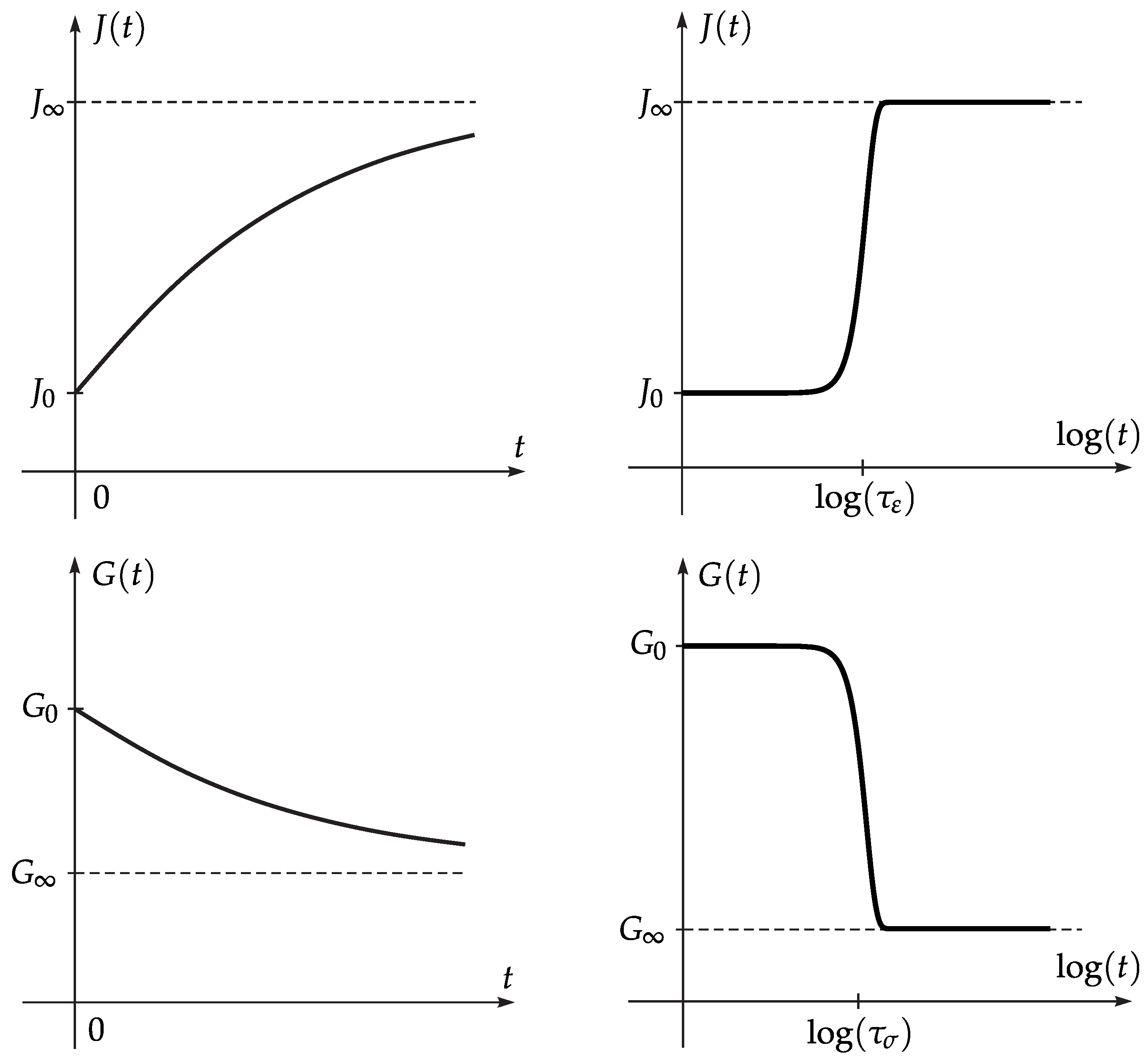
Figure 3.
Zener model.
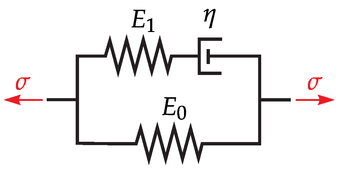
Figure 4.
Springpot (left) and fractional Zener model (right).
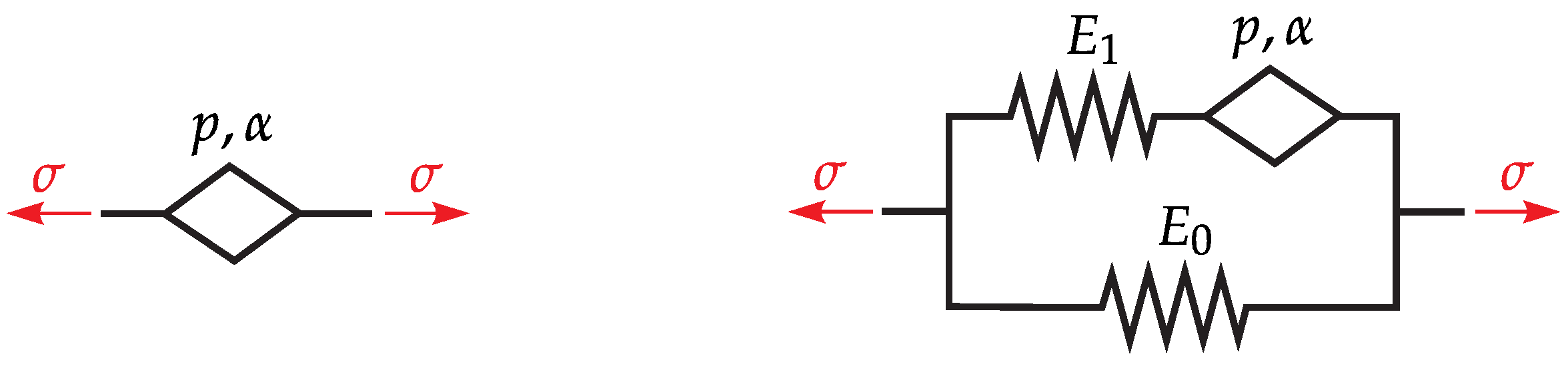
Figure 5.
Creep function of a fractional Zener model for , and various values of .
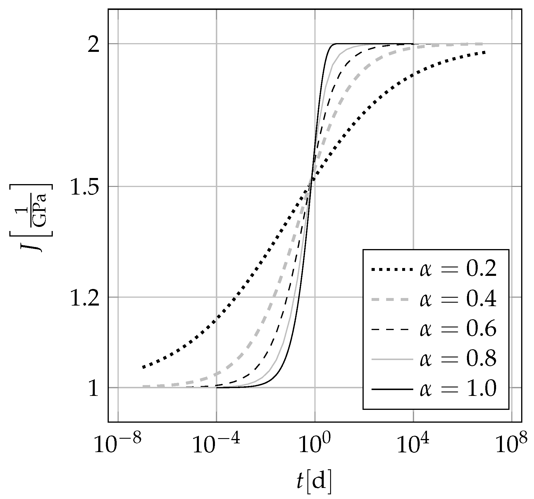
Figure 6.
Fractional Zener model.

Figure 7.
Fractional viscoelastic rod (left) described as a two-node one-dimensional finite element (right).
Figure 7.
Fractional viscoelastic rod (left) described as a two-node one-dimensional finite element (right).
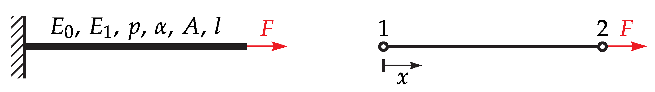

Figure 9.
Fractional viscoelastic plate element in undeformed (left) and deformed configuration (right).
Figure 9.
Fractional viscoelastic plate element in undeformed (left) and deformed configuration (right).


Publisher’s Note: MDPI stays neutral with regard to jurisdictional claims in published maps and institutional affiliations. |
© 2021 by the authors. Licensee MDPI, Basel, Switzerland. This article is an open access article distributed under the terms and conditions of the Creative Commons Attribution (CC BY) license (https://creativecommons.org/licenses/by/4.0/).
Share and Cite
MDPI and ACS Style
Hinze, M.; Schmidt, A.; Leine, R.I. Finite Element Formulation of Fractional Constitutive Laws Using the Reformulated Infinite State Representation. Fractal Fract. 2021, 5, 132. https://doi.org/10.3390/fractalfract5030132
AMA Style
Hinze M, Schmidt A, Leine RI. Finite Element Formulation of Fractional Constitutive Laws Using the Reformulated Infinite State Representation. Fractal and Fractional. 2021; 5(3):132. https://doi.org/10.3390/fractalfract5030132
Chicago/Turabian StyleHinze, Matthias, André Schmidt, and Remco I. Leine. 2021. "Finite Element Formulation of Fractional Constitutive Laws Using the Reformulated Infinite State Representation" Fractal and Fractional 5, no. 3: 132. https://doi.org/10.3390/fractalfract5030132