Article

A Mathematical Study of a Coronavirus Model with the Caputo Fractional-Order Derivative

1
Biomathematics Laboratory, Univ. Sidi Bel-Abbes, P.B. 89, Sidi Bel-Abbes 22000, Algeria
2
Dipartimento di Matematica “Giuseppe Peano”, Università di Torino, via Carlo Alberto 10, 10123 Torino, Italy
*
Author to whom correspondence should be addressed.
Member of the INdAM research group GNCS.
Fractal Fract. 2021, 5(3), 87; https://doi.org/10.3390/fractalfract5030087
Submission received: 15 June 2021 / Revised: 27 July 2021 / Accepted: 28 July 2021 / Published: 3 August 2021
(This article belongs to the Special Issue Fractal Functions and Applications)

Abstract

:
In this work, we introduce a minimal model for the current pandemic. It incorporates the basic compartments: exposed, and both symptomatic and asymptomatic infected. The dynamical system is formulated by means of fractional operators. The model equilibria are analyzed. The theoretical results indicate that their stability behavior is the same as for the corresponding system formulated via standard derivatives. This suggests that, at least in this case for the model presented here, the memory effects contained in the fractional operators apparently do not seem to play a relevant role. The numerical simulations instead reveal that the order of the fractional derivative has a definite influence on both the equilibrium population levels and the speed at which they are attained.

1. Introduction

Among the new tools that have recently come into the limelight in scientific research, fractional derivatives play an important role, in view of the fact that, in a sense, they embed memory effects in dynamical systems [1,2,3,4]. This concept has been successfully applied in mathematical physics [5], but more recently it has also been used in other contexts. In the biological framework, ecological models incorporating this type of operator have been introduced in [6], and for epidemic situations, in [7]. In view of the COVID-19 pandemic that has been affecting humanity for almost two years, in the last months several papers have been published on this topic. Some of them attempt to set up and analyze models for this epidemic based on the concept of fractional derivatives.
The simplest epidemiological model, SI, consists of two classes, namely susceptibles S and infectives I. If possible disease recovery is allowed, the class of healed individuals is introduced as R. These individuals are immune from the disease, at least temporarily. The model thus becomes type SIR. If, additionally, the recovered individuals lose disease immunity, they again become prone to being infected and thus they return to the class of susceptibles. In such cases, therefore, disease relapses are allowed, and the SIRS model is obtained. A further step forward consists of introducing another compartment, hosting the individuals that have been exposed to the disease. It is indeed well-known that, in the case of measles, individuals that have contracted the disease do not show symptoms until about at least a week after being infected. Meanwhile, they are very much able to transmit the disease, especially in the very first few days after infection. The exposed class therefore has paramount importance in transmissible disease modeling. The simplest nontrivial compartment model that shows this feature is the SEIR model. It has been taken into consideration, together with a fractional derivative approach, in [8,9]. Reference [10] also considers this formulation, but in addition time delays are explicitly built into the model. Another extension of the SEIR system is considered in [11], where the class P of “deprived and marginalised” individuals is also considered. The latter are individuals that are less able to cope with strict distancing measures and therefore contribute to the further spread of the disease. Apparently, they are “recruited” from the infected by a simple linear transition. In other words, the surviving infected exit this class either by recovering or by becoming part of P. In [12], instead, three additional classes are introduced, thereby forming the SEIQRDP model. Apart from the class D of deceased individuals, quarantined individuals Q are introduced, as well as the “insusceptible”, P. In the model, disease mortality is allowed only among quarantined, thereby most likely implying that infected that die of the disease are accounted for as having been recognized as disease carriers, and therefore put in isolation before dying. The Atagana–Baleanu fractional derivative is employed instead of the Caputo fractional derivative in [13]. Here, the infected may migrate to the quarantined Q class. Individuals in isolation may possibly become confirmed cases and therefore are lumped into the new class C. Notably, individuals belonging to both Q and C classes are assumed not to be able to disseminate the disease further, which may be a strong assumption. In Italy, at least in the early phases of the pandemic, most of the contagions involved doctors and nurses working in hospitals. This indicates that virus leakage was nevertheless possible in supposedly confined environments. After collecting data for various compartments from two countries, in [14] parameters are estimated, on the basis of which, initially a standard dynamical system and later on some fractional models, are built. In particular, the Caputo, Caputo–Fabrizio, Atangana–Baleanu and the fractal–fractional nonlocal operators are employed. Five classes of infected are considered, of which the first one essentially represents the exposed in our above terminology. The remaining ones consider symptomatic individuals that have or have not been tested and found to be positive or not. In [15], again the same previous five classes of infected individuals are considered, those having been tested or not, or those under treatment. The model also introduces a time-dependent transmission rate that tries to incorporate the social distancing measures, including the wearing of masks, and social contacts restrictions, that is, shop closures, curfew and so forth. This attempts to model the ways of fighting the epidemic diffusion that have been enforced by many governments worldwide, although the implementation times differed from country to country. Specifically, in [15], a model is proposed that extends the possible disease transmission mechanism of [14] to two other compartments which were not able to spread it. In addition to the equilibria analysis, a numerical scheme for the integration of the fractional system is developed. In both [14,15], the major novelty at the modeling level appears to be the introduction of the compartment of the vaccinated, V. In [16], an early model for treatment is also formulated using standard derivatives.
In all the papers considered above, however, no real asymptomatic class appears in the model. By this terminology, we mean people that are unrecognized carriers, in that they do not show symptoms. This class has enormous importance, given the fact that individuals in it believe that are not infectious and therefore think that they may mingle without restraint with susceptibles. However, not being recognized as disease-carriers, they contribute to the fast diffusion of the epidemic. A model with standard derivatives taking asymptomatics into account has been formulated in [17]. Symptomatic and asymptomatic infectious are partitioned into two different classes. The model is formulated via standard derivatives. Instead, in [18] a fractional operator model is presented, but the main aim of the paper consists of devising a suitable stable numerical scheme, which essentially relies on the use of the Laplace transform. The basic reproduction number is evaluated and, if smaller than one, it is shown that the epidemic is eradicated. Parameters for the simulations are taken from the literature or estimated by data fitting. The asymptomatic class is also considered in [19], where the main aim is the study of a numerical algorithm based on the Riesz wavelets is proposed.
In [20], quarantined individuals—coming from the exposed class, the symptomatic and asymptomatic infected, the isolated and treated—are considered in addition to the standard classes of the SEIR model. Notably, the model does not seem to account for disease mortality. For infected I the parameter ρ , according to the parameter list, should be interpreted to be the same as γ . It describes the migration from class I to treatment. At least both the infected and treated individuals should experience disease mortality. Indeed, if by the term “treated” the authors mean hospitalized, not including disease mortality does not appear to match observations. As a matter of fact, in the case of covid, hospitalized mortality has had a very big impact on societies worldwide. A similar remark may perhaps be made on the class P of “isolated” individuals into which the “quarantined” (being so after exposure) and infected migrate. After all, these people are still affected by the disease. In the model, the isolated and quarantined are assumed to be able to propagate the disease. However, treated individuals are not. In such cases, the same remark on the Italian hospitals’ situation mentioned above may apply. The paper investigates the existence of the solutions and the feasibility and stability of the system equilibria.
We have therefore chosen a simple model that is formulated via fractional derivatives in the line of the above research lines. It includes only the basic epidemiological classes, because the aim of modeling is to elucidate, if possible, how very complex behaviors are generated, using the minimal feasible assumptions. These must contain the basic mechanisms underlying the variables’ relationships, but should not remove the system’s basic features (Occam’s razor).
The model we propose differs in some more important or smaller aspects from each one of the systems presented in the above papers. In some cases it is simpler, which may be a shortcoming if real data need to be analyzed. On the other hand, however, it may represent an advantage in that it is well-known that minimal models sometimes help in highlighting system features whose real origin may be obscured in more complicated ones.
This paper is organized as follows. The next Section 2 contains the model description. The basic analytical properties of the system are presented in Section 3. A numerical simulation is presented in Section 4 together with a brief final discussion.

2. Material and Methods

We consider the following fractional-order epidemiological model incorporating a spread of corona virus. We consider the following classes of individuals: susceptibles S, namely the individuals who have not yet been exposed to the virus; exposed E, people who have been infected by the virus but are in the incubation period, in which they cannot yet spread the disease; symptomatic infected I, individuals that manifest symptoms and can communicate the disease; asymptomatic infected A, those persons that can communicate the disease even without having explicit symptoms; the removed class R, which includes the people that recovered from the disease. We further let N ( t ) denote the total population. Thus, N ( t ) = S ( t ) + E ( t ) + I ( t ) + A ( t ) + R ( t ) . The model reads as follows:
D q S ( t ) = Λ β I S ( I + k A ) d p S , D q E ( t ) = β I S ( I + k A ) ( 1 α ) ω p E α ω p E d p E , D q I ( t ) = ( 1 α ) ω p E ( γ p + d p + μ ) I + ξ A , D q A ( t ) = α ω p E ( γ p + d p + ν ) A ξ A , D q R ( t ) = γ p I + γ p A d p R ,
where D q is the standard Caputo differentiation with q ( 0 , 1 ) . For the benefit of the reader, we recall the definition of the Caputo fractional derivative of order q [1,2]:
D q x ( t ) = 1 Γ ( n q ) 0 t ( t s ) n q 1 x ( n ) ( s ) d s , n 1 < q < n , n N .
In the above model, all individuals experience natural mortality at rate d p ; susceptibles are recruited at constant rate Λ , these being the only two demographic features of the model. The epidemic part of the model considers disease transmission among susceptibles and both types of infected, at rate β I , through mass action. Note that the factor k modulates the possible difference in the ability to spread the disease from asymptomatic people versus symptomatic ones. After contagion, a susceptible migrates into the class of the exposed, from which, after activation of the disease, it moves on to the infected compartments, at possibly different rates ω p and ω p ; α instead tells the proportion of exposed that will never show symptoms, that is, they move to class A. From this class, at rate ξ , individuals may still be able to become symptomatic and migrate to the I class. Both types of infected individuals may recover at rates γ p and γ p and are subject to disease-related mortality, for which we assume two possibly different rates, μ for symptomatic and ν for asymptomatic people. All the parameters are non negative and their meaning is summarized in Table 1. The basic mechanisms underlying the model are shown in Figure 1.
The system (1) is completed by the following initial conditions
S ( 0 ) 0 , E ( 0 ) 0 , I ( 0 ) 0 , A ( 0 ) 0 , and R ( 0 ) 0 .

3. Results

This section studies the existence, uniqueness, non-negativity and boundedness of the solutions of a fractional order epidemiological model (1). In addition, the stability analysis of fractional order epidemiological model (1) is also performed.

3.1. Existence and Uniqueness

The sufficient condition for the existence and uniqueness of the solution of a fractional order system (1) are as follows:
Theorem 1.
For each non-negative initial conditions, there exists a unique solution of fractional order system (1).
Proof. 
We seek a sufficient condition for the existence and uniqueness of the solutions of fractional order system (1) in the region Ω × ( 0 , T ] where
Ω = { ( x , y , z , u , v ) R 2 : max ( | x | , | y | , | z | , | u | , | v | ) ρ } .
The approach used in [6] is adopted. Consider a mapping
G ( X ) = ( G 1 ( X ) , G 2 ( X ) , G 3 ( X ) , G 4 ( X ) , G 5 ( X ) )
and
G 1 ( X ) = Λ β I x ( z + k u ) d p x , G 2 ( X ) = β I x ( z + k u ) ( 1 α ) ω p y α ω p y d p y , G 3 ( X ) = ( 1 α ) ω p y ( γ p + d p + μ ) z + ξ u , G 4 ( X ) = α ω p y ( γ p + d p + ν ) u ξ u , G 5 ( X ) = γ p z + γ p u d p v .
For any X, X ¯ , it follows from (3) that
G ( X ) G ( X ¯ ) = G 1 ( X ) G 1 ( X ¯ ) + + G 5 ( X ) G 5 ( X ¯ ) = Λ β I x ( z + k u ) d p x Λ + β I x ¯ ( z ¯ + k u ¯ ) + d p x ¯ + β I x ( z + k u ) [ ( 1 α ) ω p + α ω p + d p ] y β I x ¯ ( z ¯ + k u ¯ ) + [ ( 1 α ) ω p + α ω p + d p ] y ¯ + ( 1 α ) ω p y ( γ p + d p + μ ) z + ξ u ( 1 α ) ω p y ¯ + ( γ p + d p + μ ) z ¯ ξ u ¯ + α ω p y ( γ p + d p + ν + ξ ) u α ω p y ¯ + ( γ p + d p + ν + ξ ) u ¯ + γ p z + γ p u d p v γ p z ¯ γ p u ¯ + d p v ¯
= β I x ( z z ¯ ) + z ¯ ( x x ¯ ) + k β I x ( u u ¯ ) + u ¯ ( x x ¯ ) + d p x x ¯ + β I x ( z z ¯ ) + z ¯ ( x x ¯ ) + k β I x ( u u ¯ ) + u ¯ ( x x ¯ ) + [ ( 1 α ) ω p + α ω p + d p ] y y ¯ + ( 1 α ) ω p y y ¯ + ( γ p + d p + μ ) z z ¯ + ξ u u ¯ + α ω p y y ¯ + ( γ p + d p + ν + ξ ) u u ¯ + γ p z z ¯ + γ p u u ¯ + d p v v ¯ [ 2 β I ρ ( 1 + k ) + d p ] x x ¯ + [ 2 ( 1 α ) ω p + 2 α ω p + d p ] y y ¯ + ( 2 β I ρ + 2 γ p + d p + μ ) z z ¯ + ( 2 k β I ρ + 2 ξ + 2 γ p + d p + ν ) u u ¯ + d p v v ¯ C X X ¯ ,
where
C = max 2 β I ρ ( 1 + k ) + d p , 2 ( 1 α ) ω p + 2 α ω p + d p , 2 β I ρ + 2 γ p + d p + μ , 2 k β I ρ + 2 ξ + 2 γ p + d p + ν .
Thus, G ( X ) satisfies the Lipschitz condition. Consequently, the existence and uniqueness of the solution of the fractional order system (1) follows. □

3.2. Non-Negativity and Boundedness

The solutions of the fractional order system (1) represent the densities of the interacting populations and must therefore be non-negative and bounded. These features are ensured by the following results.
Theorem 2.
All the solutions of fractional order system (1), which start in R + 5 are uniformly bounded and non-negative.
Proof. 
We follow the approach used by [6]. Define the function N ( t ) = S ( t ) + E ( t ) + I ( t ) + A ( t ) + R ( t ) . Hence, for each d p > 0 ,
D q N ( t ) + d p N ( t ) = Λ β I S ( I + k A ) d p S + β I S ( I + k A ) ( 1 α ) ω p E α ω p E d p E + ( 1 α ) ω p E ( γ p + d p + μ ) I + ξ A + α ω p E ( γ p + d p + ν ) A ξ A + γ p I + γ p A d p R + d p ( S ( t ) + E ( t ) + I ( t ) + A ( t ) + R ( t ) ) = Λ μ I ν A Λ .
By using the standard comparison theorem for fractional order [21],
N ( t ) N ( 0 ) E q d p ( t ) q + Λ ( t ) q E q , q + 1 d p ( t ) q ,
where E q is the Mittag–Leffler function. According to Lemma 5 and Corollary 6 in [21],
N ( t ) Λ d p , t +
Therefore, all the solutions of fractional order system (1) starting in R + 5 are confined to the region Σ , where
Σ = { ( S , E , I , A , R ) R + 5 : N ( t ) Λ d p + ϵ , ϵ > 0 } .
Next, we show that the solutions of the fractional order system (1) are non-negative.
From the first equation of system (1) we have
D q S ( t ) = Λ β I S ( I + k A ) d p S [ β I ( I + k A ) + d p ] S [ β I ( 1 + k ) Λ d p + d p ] S C 1 S ,
where C 1 = β I ( 1 + k ) Λ d p + d p . According to the standard comparison theorem for fractional order [21], and the positivity of the Mittag–Leffler function E q , 1 ( t ) > 0 , for any q ( 0 , 1 ) [22],
S S ( 0 ) E q , 1 ( C 1 t q ) S 0 .
From the second equation of system (1) we find
D q E ( t ) = β I S ( I + k A ) ( 1 α ) ω p E α ω p E d p E [ ( 1 α ) ω p + α ω p + d p ] E C 2 E ,
where C 2 = ( 1 α ) ω p + α ω p + d p . Therefore,
E E ( 0 ) E q , 1 ( C 2 t q ) E 0 .
From the third equation of system (1) we get
D q I ( t ) = ( 1 α ) ω p E ( γ p + d p + μ ) I + ξ A ( γ p + d p + μ ) I C 3 I ,
where C 3 = γ p + d p + μ . Therefore,
I I ( 0 ) E q , 1 ( C 3 t q ) I 0 .
From the fourth equation of system (1) we obtain
D q A ( t ) = α ω p E ( γ p + d p + ν ) A ξ A ( γ p + d p + ν + ξ ) A C 4 A ,
where C 4 = γ p + d p + ν + ξ . Therefore,
A A ( 0 ) E q , 1 ( C 4 t q ) A 0 .
From the last equation of system (1) we have
D q R ( t ) = γ p I + γ p A d p R γ p I + γ p A d p R d p R .
Therefore,
R R ( 0 ) E q , 1 ( d p t q ) R 0 .
Thus, it has been proved that the solutions of system (1) are non-negative. □

3.3. Equilibrium Points and Local Stability

In this section, we investigate the local stability of equilibrium points. The fractional-order system (1) has the following equilibrium points:
  • The coronavirus-free equilibrium P 0 ( S 0 , 0 , 0 , 0 , 0 ) , where S 0 = Λ d p . It is always feasible.
  • The coronavirus-symptomatic-infected-free equilibrium P I ( S I , E I , 0 , A I , R I ) , which is feasible if
    Λ > d p B T H T k β I ω p , α = 1 and ξ = 0 ,
    where
    E I = 1 B T Λ d p B T H T k β I ω p , S I = Λ B T E * d p , A I = ω p H T E I , R I = γ p d p ω p H T E I ,
    and
    B T = ( 1 α ) ω p + α ω p + d p , C T = γ p + μ + d p , D T = ξ + k C T , H T = γ p + ν + ξ + d p .
  • The coronavirus endemic equilibrium P * ( S * , E * , I * , A * , R * ) , which is feasible if
    Λ > d p B T C T H T β I ( 1 α ) ω p H T + α ω p D T , and   either α 1 or ξ 0 ,
    where
    E * = 1 B T Λ d p B T C T H T β I ( 1 α ) ω p H T + α ω p D T , S * = Λ B T E * d p ,
    I * = ( 1 α ) ω p H T + α ω p ξ C T H T E * , A * = α ω p H T E *
    R * = γ p d p ( 1 α ) ω p H T + α ω p ξ C T H T + γ p d p α ω p H T E * .

3.4. The Basic Reproduction Number

The basic reproduction number R 0 for our fractional model is found using the next generation matrix method [23].
The reduced system may be written in compact form as: D q X = F ( X ) V ( X ) , where X = ( E , I , A )
F ( E , I , A ) = β I S ( I + k A ) 0 0 , V ( E , I , A ) = ( 1 α ) ω p E α ω p E d p E ( 1 α ) ω p E ( γ p + d p + μ ) I + ξ A α ω p E ( γ p + d p + ν ) A ξ A .
The Jacobian matrices of F ( X ) and V ( X ) at the disease-free equilibrium point P 0 are
J F ( P 0 ) = 0 β I S 0 β I S 0 k 0 0 0 0 0 0
and
J V ( P 0 ) = B T 0 0 ( 1 α ) ω p C T ξ α ω p 0 H T .
We find that
J V 1 ( P 0 ) = 1 B T 0 0 [ ( 1 α ) ω p H T + α ω p ξ ] C T B T H T 1 C T ξ C T H T α ω p B T H T 0 1 H T .
The next generation matrix is
J F ( P 0 ) J V 1 ( P 0 ) = β I S 0 [ ( 1 α ) ω p H T + α ω p D T ] C T B T H T β I S 0 1 C T β I S 0 D T C T H T 0 0 0 0 0 0 .
Thus
R 0 = ρ ( J F ( P 0 ) J V 1 ( P 0 ) ) = β I S 0 [ ( 1 α ) ω p H T + α ω p D T ] C T B T H T .
Next, we will discuss the stability of the equilibrium points of system (1). At the point P ( S , E , I , A , R ) , the Jacobian matrix of system (1) is given by
J ( P ) = β I ( I + k A ) d p 0 β I S β I S k 0 β I ( I + k A ) B T β I S β I S k 0 0 ( 1 α ) ω p C T ξ 0 0 α ω p 0 H T 0 0 0 γ p γ p d p .
Using the Jacobian matrix (12) and the Matignon condition [4,7], the local stability of the equilibrium points of the fractional-order system (1) is investigated. We have the following results.
Theorem 3.
The coronavirus-free equilibrium P 0 of the fractional-order system (1) is locally asymptotically stable if
Λ < d p β I B T C T H T ( 1 α ) ω p H T + α ω p D T , i . e . , R 0 = β I S 0 ( 1 α ) ω p H T + α ω p D T C T B T H T < 1 ,
and unstable if
Λ > d p β I B T C T H T ( 1 α ) ω p H T + α ω p D T , ( i . e . , R 0 > 1 ) .
Here, recall that R 0 denotes the basic reproduction number.
Proof. 
Letting
a 2 = B T + C T + H T , a 1 = H T [ B T + C T ] + B T C T β I S 0 ( ( 1 α ) ω p + k α ω p ) a 0 = B T C T H T β I S 0 ( 1 α ) ω p H T + α ω p D T ,
the Jacobian matrix (12) around the coronavirus-free equilibrium P 0 is
J ( P 0 ) = d p 0 β I Λ d p k β I Λ d p 0 0 B T β I Λ d p k β I Λ d p 0 0 ( 1 α ) ω p C T ξ 0 0 α ω p 0 H T 0 0 0 γ p γ p d p .
The eigenvalues of the Jacobian matrix J ( P 0 ) around the coronavirus-free equilibrium P 0 are λ 1 = d p of multiplicity order two and the roots of the characteristic polynomial of the minor matrix of J ( P 0 ) given by
C ( λ ) = λ 3 + a 2 λ 2 + a 1 λ + a 0 = 0 ,
where a i , i = 0 , , 2 are given in (15).
It is evident that a 2 > 0 . From condition (13), the following equations are also satisfied:
a 0 = B T C T H T β I S 0 ( 1 α ) ω p H T + α ω p D T = β I d p ( 1 α ) ω p H T + α ω p D T d p β I B T C T H T ( 1 α ) ω p H T + α ω p D T Λ > 0 ,
( 1 α ) ω p H T + α ω p D T a 1 = [ H T ( B T + C T ) + B T C T ] ( 1 α ) ω p H T + α ω p D T β I S 0 ( 1 α ) ω p H T + α ω p D T [ ( 1 α ) ω p + k α ω p ] = [ H T ( B T + C T ) + B T C T ] ( 1 α ) ω p H T + α ω p D T + [ a 0 B T C T H T ] [ ( 1 α ) ω p + k α ω p ] = H T ( B T + C T ) ( 1 α ) ω p H T + ( H T C T + B T C T ) α ω p ξ + a 0 [ ( 1 α ) ω p + k α ω p ] > 0
and
( 1 α ) ω p H T + α ω p D T a 1 a 2 = H T ( B T + C T ) ( 1 α ) ω p H T a 2 + ( H T C T + B T C T ) α ω p ξ a 2 + a 0 [ ( 1 α ) ω p + k α ω p ] a 2 = H T ( B T + C T ) ( 1 α ) ω p H T a 2 + ( H T C T + B T C T ) α ω p ξ a 2 + a 0 ( 1 α ) ω p ( B T + C T + H T ) + a 0 k α ω p ( B T + C T + H T ) > B T C T α ω p ξ a 2 + a 0 ( 1 α ) ω p H T + a 0 α ω p ( k C T + ξ ) a 0 α ω p ξ > B T C T H T α ω p ξ + a 0 [ ( 1 α ) ω p H T + α ω p D T ] B T C T H T α ω p ξ = a 0 [ ( 1 α ) ω p H T + α ω p D T ] .
Thus, a i > 0 , i = 0 , , 2 and a 2 a 1 > a 0 .
From the Routh–Hurwitz criterion, all the roots λ i of the characteristic Equation (16) have negative real parts. By using Matignon’s condition [4,7], it can be observed that | a r g ( λ i ) | > q π 2 for all 0 < q < 1 . Therefore, the coronavirus-free equilibrium point P 0 is locally asymptotically stable if condition (13) is satisfied. Under condition (14), we have a 0 < 0 and lim λ + C ( λ ) = + . Then a positive real root λ * > 0 of the characteristic Equation (16) exists; from Matignon’s condition [4,7], it can be observed that | a r g ( λ * ) | = 0 < q π 2 for all 0 < q < 1 . Thus, the coronavirus-free equilibrium point P 0 is unstable. □
The coronavirus-free equilibrium point P 0 is locally asymptotically stable when the coronavirus-symptomatic-free equilibrium P I and the coronavirus endemic equilibrium P * do not exist.
Since we can deduce the stability of coronavirus symptomatic infected-free equilibrium P I from the stability of coronavirus endemic equilibrium P * by taking α = 1 and ξ = 0 , the stability of the coronavirus endemic equilibrium P * is now discussed.
Theorem 4.
Let
c 3 = β I ( I * + k A * ) + d p + H T + B T + C T > 0 , c 2 = [ β I ( I * + k A * ) + d p ] ( H T + B T + C T ) + B T C T + H T ( B T + C T ) [ α ω p k + ( 1 α ) ω p ] β I S * , c 1 = [ β I ( I * + k A * ) + d p ] [ B T C T + H T ( B T + C T ) ] + H T B T C T [ α ω p ( k d p + D T ) + ( 1 α ) ω p ( d p + H T ) ] β I S * , c 0 = [ β I ( I * + k A * ) + d p ] H T B T C T d p [ α ω p D T + ( 1 α ) ω p H T ] β I S * .
The coronavirus endemic equilibrium P * of the fractional-order system (1) is locally asymptotically stable if
Λ > d p β I B T C T H T ( 1 α ) ω p H T + α ω p D T , ( i . e . , R 0 > 1 ) .
Proof. 
At the coronavirus endemic equilibrium P * , the Jacobian matrix (12) is given by
J ( P * ) = β I ( I * + k A * ) d p 0 β I S * β I S * k 0 β I ( I * + k A * ) B T β I S * β I S * k 0 0 ( 1 α ) ω p C T ξ 0 0 α ω p 0 H T 0 0 0 γ p γ p d p .
The eigenvalues of the Jacobian matrix J ( P * ) at the equilibrium P * are d p < 0 and the roots of the characteristic polynomial arising from the remaining minor of order four:
λ 4 + c 3 λ 3 + c 2 λ 2 + c 1 λ + c 0 = 0 ,
where c i , i = 0 , , 3 are given in (17).
It is evident that c 3 > 0 . From condition (18), the following inequalities on the coefficients are also satisfied.
c 0 = [ β I ( I * + k A * ) + d p ] H T B T C T β I [ ( 1 α ) ω p H T + α ω p D T ] d p S * = β I ( 1 α ) ω p H T + α ω p ( ξ + k C T ) B T E * + d p H T C T B T β I [ ( 1 α ) ω p H T + α ω p D T ] ( Λ B T E * ) = β I ( 1 α ) ω p H T + α ω p D T 2 B T E * + d p H T C T B T β I [ ( 1 α ) ω p H T + α ω p D T ] Λ = β I ( 1 α ) ω p H T + α ω p D T B T E * > 0 ,
c 1 = [ β I ( I * + k A * ) + d p ] [ B T C T + H T ( B T + C T ) ] + H T B T C T [ ( 1 α ) ω p ( d p + H T ) + α ω p ( k d p + D T ) ] β I S * = β I ( 1 α ) ω p H T + α ω p D T C T H T E * + d p [ B T C T + H T ( B T + C T ) ] β I [ ( 1 α ) ω p + α ω p k ] ( Λ B T E * ) = β I ( 1 α ) ω p H T ( B T + C T ) C T + α ω p ξ B T C T + α ω p D T ( B T + H T ) H T E * + d p [ B T C T + H T ( B T + C T ) ] β I [ ( 1 α ) ω p + α ω p k ] ( Λ 2 B T E * ) = β I ( 1 α ) ω p H T ( B T + C T ) C T + α ω p ξ B T C T + α ω p D T ( B T + H T ) H T E * + d p [ B T C T + H T ( B T + C T ) ] β I [ ( 1 α ) ω p + α ω p k ] 2 d p B T C T H T β I ( 1 α ) ω p H T + α ω p D T Λ = β I [ ( 1 α ) ω p H T + α ω p D T ] C T H T + B T ( C T + H T ) C T H T E * + d p ( B T + C T ) H T 2 ( 1 α ) ω p + H T B T α ω p ξ + C T ( B T + H T ) α ω p D T ( 1 α ) ω p H T + α ω p D T > 0 ,
c 2 = [ β I ( I * + k A * ) + d p ] ( H T + B T + C T ) + B T C T + H T ( B T + C T ) [ α ω p k + ( 1 α ) ω p ] β I S * = β I ( 1 α ) ω p H T + α ω p D T C T H T E * + d p ( H T + B T + C T ) + B T C T + H T ( B T + C T ) [ α ω p k + ( 1 α ) ω p ] β I Λ B T E * d p = β I ( 1 α ) ω p ( H T + B T ) C T + α ω p ξ ( H T + B T + C T ) C T H T + α ω p k ( B T + C T ) H T E * + d p ( H T + B T + C T ) + B T C T + H T ( B T + C T ) + β I [ ( 1 α ) ω p + α ω p k ] ( d p + B T ) E * Λ d p = β I ( 1 α ) ω p ( H T + B T ) C T + α ω p ξ ( H T + B T + C T ) C T H T + α ω p k ( B T + C T ) H T E * + d p ( H T + B T + C T ) + B T C T + H T ( B T + C T ) + β I [ ( 1 α ) ω p + α ω p k ] B T Λ ( d p + B T ) B T C T H T β I ( 1 α ) ω p H T + α ω p D T = β I ( B T + C T + H T ) ( 1 α ) ω p H T + α ω p D T C T H T E * + d p ( H T + B T + C T ) + C T H T + B T ( 1 α ) ω p H T 2 + H T α ω p ξ + α ω p C T D T ( 1 α ) ω p H T + α ω p D T > 0
and
c 1 ( c 3 c 2 c 1 ) = β I ( 1 α ) ω p H T + α ω p D T C T H T E * c 1 c 2 + β I ( H T + C T + d p ) H T + C T ( C T + d p ) × ( 1 α ) ω p H T + α ω p D T C T H T E * c 1 + β I ( H T + B T + C T + d p ) B T ( 1 α ) ω p H T + α ω p D T C T H T E * c 1 + ( H T + B T + C T ) ( H T + B T + C T + d p ) d p c 1 + C T H T ( C T + H T + B T ) c 1 + B T ( B T + C T + H T ) [ ( 1 α ) ω p H T 2 + α ω p C T D T ] + α ω p ξ H T ( 1 α ) ω p H T + α ω p D T c 1 > β I 3 B T ( 1 α ) ω p H T + α ω p D T ( 1 α ) ω p H T + α ω p D T C T H T 2 E * 3 + 2 β I 2 B T ( d p + H T + B T + C T ) [ ( 1 α ) ω p H T + α ω p D T ] ( 1 α ) ω p H T + α ω p D T C T H T E * 2 + β I B T ( d p + H T + B T + C T ) 2 ( 1 α ) ω p H T + α ω p D T E * = c 0 c 3 2 .
Thus, c i > 0 , i = 0 , , 3 and c 1 ( c 3 c 2 c 1 ) > c 0 c 3 2 . Then, according to the Routh–Hurwitz criterion, all the roots of the characteristic Equation (19) have negative real parts. By using Matignon’s condition [4,7], it can be observed that | a r g ( λ 1 ) | = π > q π 2 for all 0 < q < 1 . Therefore, the coronavirus endemic equilibrium point P * is locally asymptotically stable if (18) is satisfied. □
From Theorem 4, we obtain the following result.
Remark 1.
Letting
b 3 = β I k A I + d p + H T + B T + C T > 0 , b 2 = [ β I k A I + d p ] ( H T + B T + C T ) + B T C T + H T ( B T + C T ) ω p k β I S I , b 1 = [ β I k A I + d p ] [ B T C T + H T ( B T + C T ) ] + H T B T C T ω p ( k d p + D T ) β I S I , b 0 = [ β I k A I + d p ] H T B T C T d p ω p D T β I S * .
The coronavirus symptomatic-infected-free equilibrium P I of the system (1) is locally asymptotically stable if
Λ > d p β I B T C T H T ω p D T , ( i . e . , R 0 > 1 ) .
Proof. 
The result can easily be deduced from Theorem 4 by taking α = 1 and ξ = 0 . □

3.5. Global Stability

The global asymptotic stability of the equilibria P 0 , P I and P * of the fractional-order system (1) is now investigated by using a suitable constructed Lyapunov function, Lemma 4.6 in [24] and Lemma 3.1 in [25].
Theorem 5.
If
Λ < d p B T C T H T β I [ ( 1 α ) ω p H T + D T α ω p ] , ( i . e . , R 0 < 1 ) ,
then the coronavirus-free equilibrium P 0 of the fractional-order system (1) is globally asymptotically stable in R + 5 .
Proof. 
First, the four equations in (1) are independent of R, therefore the last equation in (1) can be omitted without loss of generality. Hence, let us consider the following function:
V 0 ( S , E , I , A ) = S S 0 S 0 ln S S 0 + E + B T [ ( 1 α ) ω p H T + D T α ω p ] ( H T I + D T A ) .
It is easily seen that the above function is non-negative and also V 0 = 0 if and only if S = S 0 , E = 0 , I = 0 and A = 0 . Further, calculating the q-order derivative of V 0 along the positive solutions of (1), we find:
D q V 0 ( S , E , I , A ) 1 S ( S S 0 ) D q S + D q E + B T ( H T D q I + D T D q A ) [ ( 1 α ) ω p H T + D T α ω p ] = 1 S ( S S 0 ) ( β I S ( I + k A ) d p ( S S 0 ) ) + β I S ( I + k A ) B T E + B T H T ( ( 1 α ) ω p E C T I + ξ A ) [ ( 1 α ) ω p H T + D T α ω p ] + B T D T ( α ω p E H T A ) [ ( 1 α ) ω p H T + D T α ω p ] = d p S ( S S 0 ) 2 + β I S 0 ( I + k A ) B T C T H T I [ ( 1 α ) ω p H T + D T α ω p ] B T ( ξ + D T ) H T A [ ( 1 α ) ω p H T + D T α ω p ] = d p S ( S S 0 ) 2 + β I S 0 B T C T H T [ ( 1 α ) ω p H T + D T α ω p ] ( I + k A ) = d p S ( S S 0 ) 2 + β I d p Λ d p B T C T H T β I [ ( 1 α ) ω p H T + D T α ω p ] ( I + k A ) .
From condition (22), we can show that the coefficient of the term I + k A in the last equality are negative. Thus, we have D q V 0 0 for all ( S , E , I , A ) R + 4 and D q V 0 = 0 if and only if ( S , E , I , A ) = ( S 0 , 0 , 0 , 0 ) . Thus, the only invariant set contained in R + 4 is { ( S 0 , 0 , 0 , 0 ) } . Hence, by Lemma 4.6 of [24], it is enough to prove the convergence of the solutions ( S , E , I , A ) to ( S 0 , 0 , 0 , 0 ) . From the last equation of (1) we can easily show that R converges also to 0. Therefore, P 0 is globally asymptotically stable in R + 5 if R 0 < 1 . □
Theorem 6.
If
Λ > d p B T H T β I k ω p , ( i . e . , R 0 > 1 ) ,
then the coronavirus-symptomatic-infected-free equilibrium P I of the fractional-order system (1) is globally asymptotically stable in R + 5 / R + × { ( 0 , 0 , 0 ) } × R + .
Proof. 
Consider the function
V 1 ( S , E , I , A ) = S S I S I ln S S I + E E I E I ln E E I + β I S I C T I + k β I S I H T A A I A I ln A A I .
This function is positive and V 1 ( S , E , I , A ) = 0 if and only if ( S , E , I , A ) = ( S I , E I , 0 , A I ) .
By calculating the q-order derivative of V 1 along the solution trajectories of system (1) and using Lemma 3.1 in [25], we obtain
D q V 1 ( S , E , I , A ) 1 S I S Λ β I S ( I + k A ) d p S + 1 E I E β I S ( I + k A ) B T E + β I S I C T C T I + k β I S I H T 1 A I A ω p E H T A = 1 S I S β I S I k A I + d p S I β I S ( I + k A ) d p S + 1 E I E β I S ( I + k A ) B T E + β I S I k A I β I S I I + k β I S I H T 1 A I A ω p E k β I S I A + k β I S I H T ω p E I = d p S S S I 2 + β I S I k A I 1 S I S β I E I S I E k β I E I S A E k β I S I H T ω p A I E A + β I S I k A I + k β I S I H T ω p E I .
Now, substituting
x = S S I , y = E E I , z = I , u = A A I ,
in inequality (24), we obtain
D q V 1 ( S , E , I , A ) d p S S S I 2 + β I S I k A I 2 1 x x u y β I S I x z y + k β I S I H T ω p E I 1 y u .
From the fourth equation of (1), we have
ω p E I H T A I = 0 .
Multiplying the Equation (25) by
k β I S I H T F 1 ( x , y , z , u ) ,
where F 1 ( x , y , z , u ) is a function to be determined later, yields
k β I S I H T ω p E I F 1 ( x , y , z , u ) β I S I k A I F 1 ( x , y , z , u ) = 0 .
Then, we obtain
D q V 1 ( S , E , I , A ) d p S S S I 2 + β I S I k A I 2 1 x x u y F 1 ( x , y , z , u ) β I S I x z y + k β I S I H T ω p E I 1 y u + F 1 ( x , y , z , u ) .
The function F 1 ( x , y , z , u ) is chosen such that the coefficient of E I is equal to zero. In this case, we obtain
F 1 ( x , y , z , u ) = y u 1 .
Thus, inequality (27) is equivalent to
D q V 1 ( S , E , I , A ) d p S S S I 2 + β I S I k A I 3 1 x x u y y u β I S I x z y .
By the arithmetic mean-geometric mean inequality we have 3 1 x x u y y u 0 for all x 0 , y 0 and u 0 . Hence D q V 1 ( S , E , I , A ) 0 , and D q V 1 ( S , E , I , A ) = 0 if and only if S = S I , I = 0 and u = y (i.e., E E I = A A I ). Since S must remain constant at S I , D q S is zero. This implies that A = A I and E = E I . Thus, by Lemma 4.6 in [24], it follows that the coronavirus-symptomatic-infected-free equilibrium P I is globally asymptotically stable in R + 5 / R + × { ( 0 , 0 , 0 ) } × R + . □
Theorem 7.
If
Λ > d p B T C T H T β I ( 1 α ) ω p H T + α ω p D T , ( i . e . , R 0 > 1 ) , a n d   e i t h e r α 1 o r ξ 0 ,
the fully endemic equilibrium P * of the fractional-order system (1) is globally asymptotically stable in R + 5 / R + × { ( 0 , 0 , 0 ) } × R + .
Proof. 
Consider the function
V 2 ( S , E , I , A ) = S S * S * ln S S * + E E * E * ln E E * + β I S * C T I I * I * ln I I * + β I S * D T C T H T A A * A * ln A A * .
This function is positive and V 2 ( S , E , I , A ) = 0 if and only if ( S , E , I , A ) = ( S * , E * , I * , A * ) .
By calculating the q-order derivative of V 2 along the solution of system (1) and using Lemma 3.1 in [25], we obtain
D q V 2 ( S , E , I , A ) 1 S * S Λ β I S ( I + k A ) d p S + 1 E * E β I S ( I + k A ) B T E + β I S * C T 1 I * I ( 1 α ) ω p E C T I + ξ A + β I S * D T C T H T 1 A * A α ω p E H T A = 1 S * S β I S * ( I * + k A * ) + d p S * β I S ( I + k A ) d p S + 1 E * E β I S ( I + k A ) B T E + β I S * ( I * + k A * ) + β I S * C T 1 I * I ( 1 α ) ω p E + ξ A β I S * C T C T I + β I S * C T [ ( 1 α ) ω p E * + ξ A * ] + β I S * D T C T H T 1 A * A α ω p E β I S * D T C T H T H T A + β I S * D T C T H T α ω p E * = d p S S S * 2 + β I S * I * 1 S * S + β I S * k A * 1 S * S β I E * S I E k β I E * S A E β I S * C T ( 1 α ) ω p I * E I β I S * C T ξ I * A I β I S * D T C T H T α ω p A * E A + β I S * ( I * + k A * ) + β I S * C T [ ( 1 α ) ω p E * + ξ A * ] + β I S * D T C T H T α ω p E * .
Now, replacing
x = S S * , y = E E * , z = I I * , u = A A * ,
in inequality (27), we obtain
D q V 2 ( S , E , I , A ) d p S S S * 2 + β I S * I * 2 1 x x z y + β I S * k A * 2 1 x x u y + β I S * C T ( 1 α ) ω p E * 1 y z + β I S * C T ξ A * 1 u z + β I S * ( k C T + ξ ) C T H T α ω p E * 1 y u .
From the third and fourth equations of (1), we have
C T I * ( 1 α ) ω p E * ξ A * = 0 ,
α ω p E * H T A * = 0 .
Multiplying the Equations (30) and (31) respectively by
β I S * C T F 2 ( x , y , z , u ) , β I S * ( k C T + ξ ) C T H T F 3 ( x , y , z , u ) ,
where F 2 ( x , y , z , u ) and F 3 ( x , y , z , u ) are functions to be determined later, yields
C T I * ( 1 α ) ω p E * ξ A * β I S * C T F 2 ( x , y , z , u ) = 0 ,
α ω p E * H T A * β I S * ( k C T + ξ ) C T H T F 3 ( x , y , z , u ) = 0 .
Then, we have
D q V 2 ( S , E , I , A ) d p S S S * 2 + β I S * I * 2 1 x x z y + F 2 ( x , y , z , u ) + β I S * k A * 2 1 x x u y F 3 ( x , y , z , u ) + β I S * C T ( 1 α ) ω p E * 1 y z F 2 ( x , y , z , u ) + β I S * C T ξ A * 1 u z F 2 ( x , y , z , u ) F 3 ( x , y , z , u ) + β I S * ( k C T + ξ ) C T H T α ω p E * 1 y u + F 3 ( x , y , z , u ) .
The functions F 2 ( x , y , z , u ) and F 3 ( x , y , z , u ) are chosen such that the coefficients of ω p E * and I * are equal to zero. In this case, we obtain
F 2 ( x , y , z , u ) = 1 x + x z y 2 ,
and
F 3 ( x , y , z , u ) = y u 1 .
Thus, inequality (35) is equivalent to
D q V 2 ( S , E , I , A ) d p S S S * 2 + β I S * k A * 3 1 x x u y y u + β I S * C T ( 1 α ) ω p E * 3 y z 1 x x z y + β I S * C T ξ A * 4 u z 1 x x z y y u .
By the arithmetic mean-geometric mean inequality we have 3 1 x x u y y u 0 , 3 y z 1 x x z y 0 and 4 u z 1 x x z y y u 0 for all x 0 , y 0 , z 0 and u 0 . Hence, D q V 1 ( S , E , I , A ) 0 , and D q V 1 ( S , E , I , A ) = 0 if and only if S = S * and u = z = y (i.e., E E * = I I * = A A * ). Since S must remain constant at S * , D q S is zero. This implies that A = A * , I = I * and E = E * . Thus, by Lemma 4.6 in [24], it follows that the fully endemic equilibrium P * is globally asymptotically stable in R + 5 / R + × { ( 0 , 0 , 0 ) } × R + . □
Remark 2.
If the initial conditions start from R + × { ( 0 , 0 , 0 ) } × R + , then the solution converges to the coronavirus-free equilibrium point P 0 .

4. Discussion

The proposed epidemic model for COVID-19 containing a fractional derivative formulation has been analyzed. The results show that the model is sound, because trajectories are confined to a compact set and the subpopulations corresponding to the various compartments into which the whole population is partitioned remain bounded. Unboundedness would indeed be biologically impossible. The model exhibits the endemic equilibrium P * at which the disease persists. It also contains the disease-free point with only susceptible individuals, P 0 , for which the pandemic is finally eradicated. This equilibrium should be the goal of the policies attempting epidemic diffusion confinement. There is also an “intermediate equilibrium”, P I , which does not contain symptomatic infected, but it still harbors the disease among the asymptomatic individuals, so that it is in reality still endemic. The susceptible-only point P 0 is incompatible with both P I and P * , the latter being unfeasible when the former is stably attained. Note also that P I is a kind of particular case of coexistence P * , which arises if asymptomatics will never develop symptoms and all the exposed migrate into the asymptomatic class. In Section 3.5, global stability for each equilibrium in suitable conditions is shown. This result is relevant but also to be expected, in view of the incompatibility of multiple equilibria discussed above.
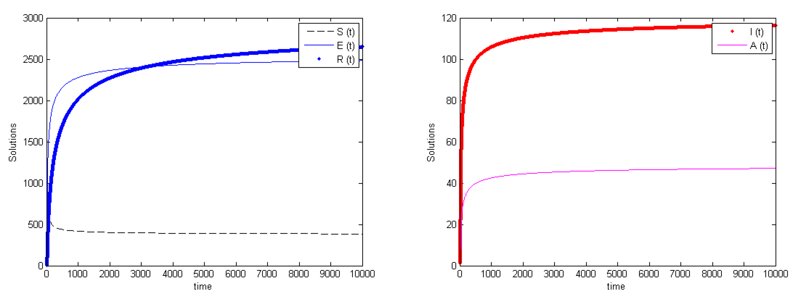
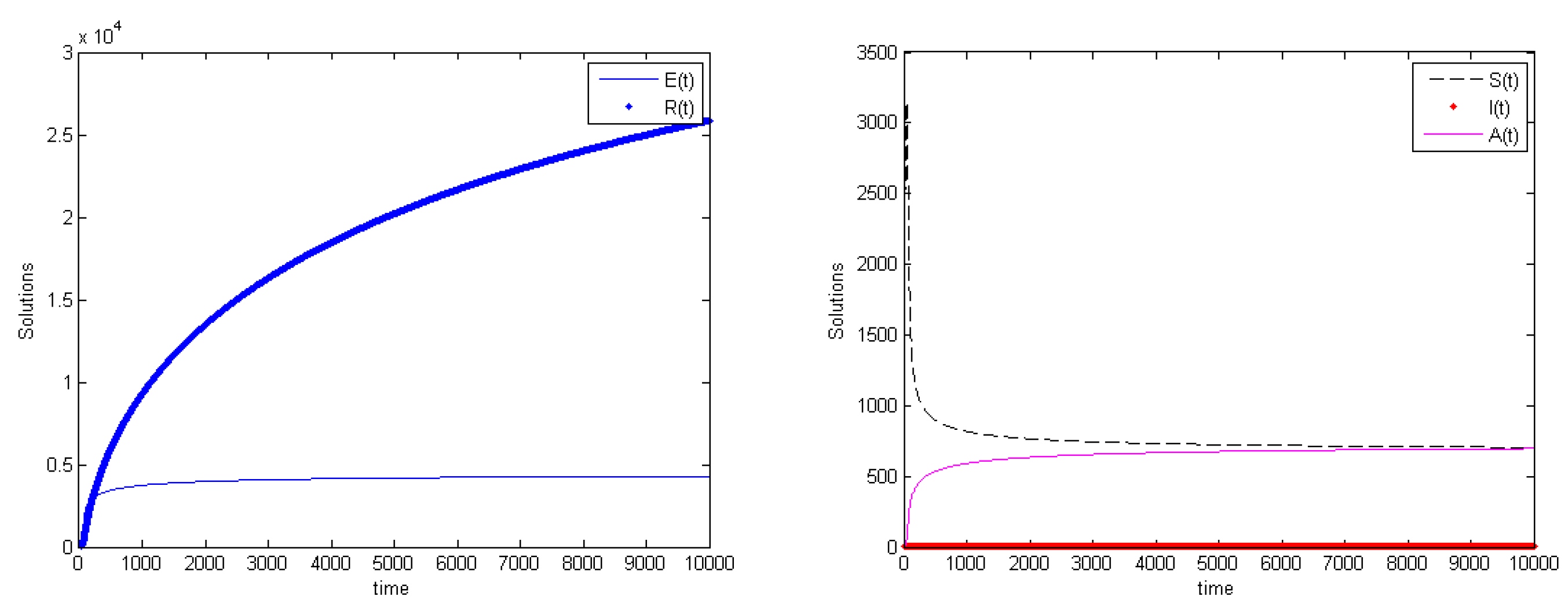
Figure 2, Figure 3 and Figure 4 show these three theoretical types of possible model behaviors. The comparison of these results with publicly available datasets on COVID-19 is not really our goal. In part, this is also due to the discussion that follows below, indicating that the population equilibrium levels change with the changes of the fractional derivative order.
Note that, of the two endemic points P * and P I , at equilibrium P I the disease remains hidden in the population. However, it still has its pernicious effects, since people will still “silently” die of it, at rate ν . In a sense, this equilibrium is worse than the explicit endemic one P * , because the latter keeps on showing to the people that the disease is not eradicated and therefore warns the population to maintain suitable safety measures.
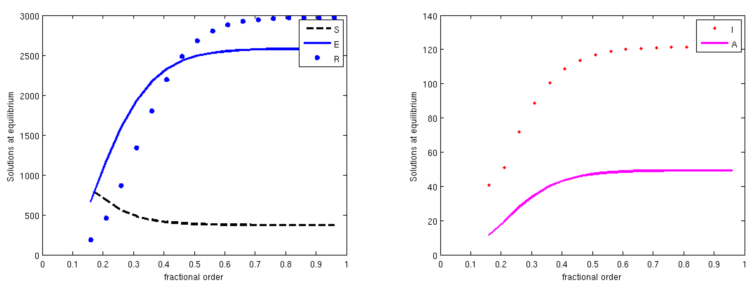
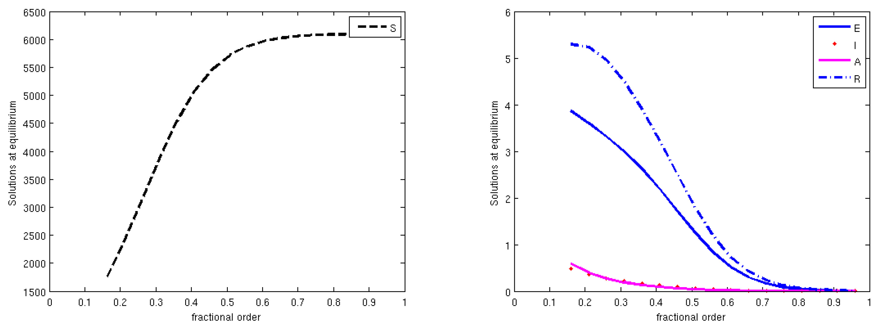
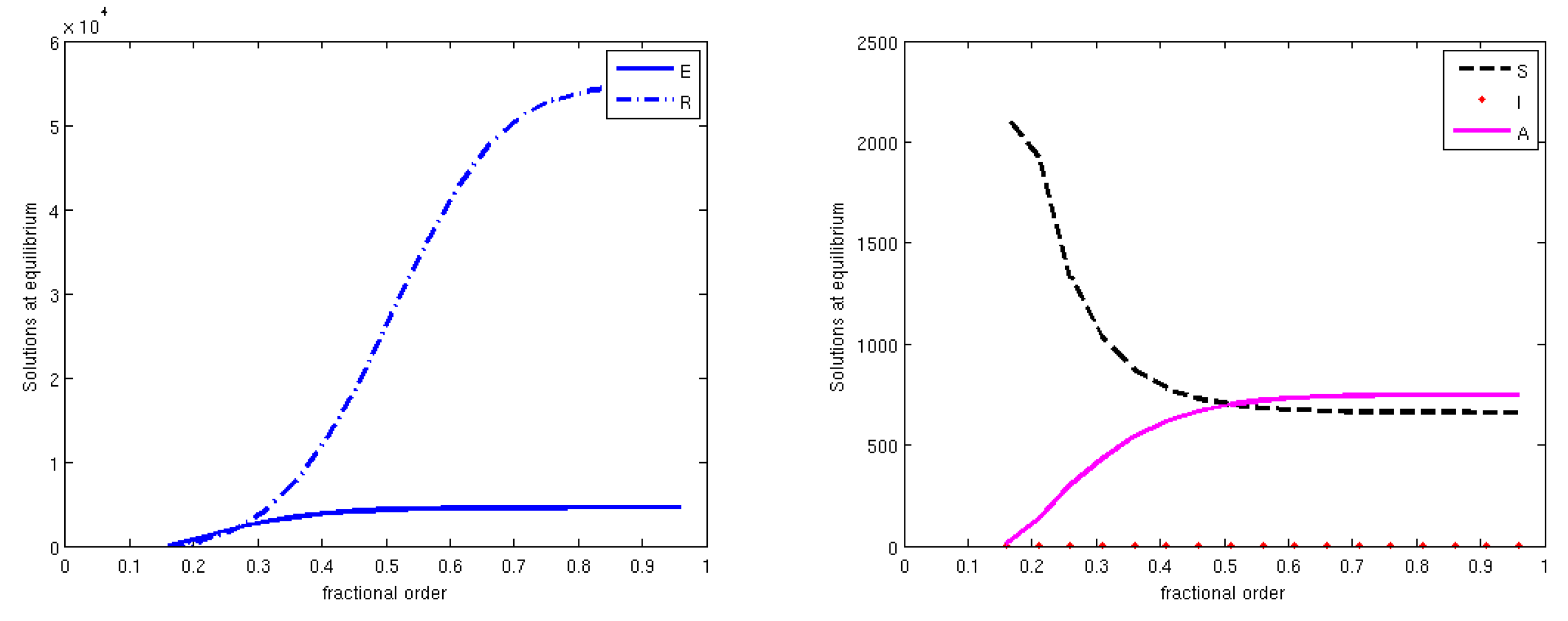
Finally, we observe that the stability results obtained analytically for the fractional operator model in this case do coincide with those of the model formulated using standard derivatives. Therefore, theoretically, the memory effects on this dynamical system are essentially scantly relevant, and the use of a classical standard formulation appears to be adequate. However, to further analyse in practice the effect of the order of the fractional derivatives, we have investigated how it may possibly affect the equilibrium levels. Simulations of the population values attained at equilibrium are also reported as a function of the fractional derivative order, in Figure 5, Figure 6 and Figure 7, which correspond to the time series of the Figure 2, Figure 3 and Figure 4 mentioned above. It is clearly seen that the order q of the fractional derivative does influence the final stage of the compartment levels. In Figure 5, for the endemic equilibrium P * , all compartments show a population decrease when q falls below 0.5 , with the exception of S, which slightly increases. The same trend is also observed for the other endemic point P I , in Figure 7, although in this case the compartments are arranged differently in the two frames, to better show the details. For the disease-free point P 0 , in Figure 6, a low value of q decrements the susceptibles and increases the other compartments. These are very small, but in fact should vanish. However, the simulations have all been carried out with the same final time T = 10,000, so that the result indicates that a low q entails a longer time for disease eradication.
A possible line of research to be pursued in the future is to compare the real-world scenario data with the simulation outcomes to assess the optimal fractional order to be used in the model, or if instead the standard derivatives are sufficient.

Author Contributions

Methodology, Y.B., M.H., A.L. and E.V.; software, simulation, M.H., A.L.; validation, Y.B., M.H., A.L. and E.V.; formal analysis, Y.B., M.H., A.L. and E.V.; writing—original draft preparation, Y.B., M.H.; writing—review and editing, M.H., E.V. All authors have read and agreed to the published version of the manuscript.

Funding

E.V. was partially funded by the local research project “Questioni attuali di approssimazione numerica e loro applicazioni” of the Dipartimento di Matematica, Universitá di Torino. This research has been undertaken within the framework of the COST Action: CA 16227—Investigation and Mathematical Analysis of Avant-garde Disease Control via Mosquito Nano-Tech-Repellents. This work was partially supported by the Ministry of Higher Education and Scientific Research of Algeria (MESRS) and General Direction of Scientific Research and Technological Development (DGRSDT) through Research Project-University Formation (PRFU: C00L03UN220120190001 and PRFU: C00L03UN220120180004).

Institutional Review Board Statement

Not applicable.

Informed Consent Statement

Not applicable.

Data Availability Statement

Not applicable.

Acknowledgments

The authors would like to thank the reviewers for their valuable comments and suggestions that greatly improved the presentation of this work.

Conflicts of Interest

The authors declare no conflict of interest.

References

  1. Diethelma, K.; Ford, N.J. Analysis of Fractional Differential Equations. J. Math. Anal. Appl. 2002, 265, 229–248. [Google Scholar] [CrossRef] [Green Version]
  2. Kilbas, A.A.; Srivastava, H.M.; Trujillo, J.J. Theory and Applications of Fractional Differential Equations; Elsevier: Amsterdam, The Netherlands, 2006. [Google Scholar]
  3. Podlubny, I. Fractional Differential Equations; Academic Press: London, UK, 1999. [Google Scholar]
  4. Petras, I. Fractional-Order Nonlinear Systems: Modeling, Analysis and Simulation; Springer: Berlin, Germany, 2011. [Google Scholar]
  5. Caputo, M. Elasticità e dissipazione (Elasticity and Dissipation); Zanichelli: Bologna, Italy, 1969. [Google Scholar]
  6. Li, H.L.; Zhang, L.; Hu, C.; Jiang, Y.L.; Teng, Z. Dynamical analysis of a fractional-order predator-prey model incorporating a prey refuge. J. Appl. Math. Comput. 2017, 54, 435–449. [Google Scholar] [CrossRef]
  7. Nugraheni, K.; Trisilowati, T.; Suryanto, A. Dynamics of a fractional order eco-epidemiological model. J. Trop. Life Sci. 2017, 7, 243–250. [Google Scholar] [CrossRef] [Green Version]
  8. Ahmad, Z.; Arif, M.; Ali, F.; Khan, I.; Nisar, K.S. A report on COVID-19 epidemic in Pakistan using SEIR fractional model. Sci. Rep. 2020, 10, 22268. [Google Scholar] [CrossRef]
  9. Panwar, V.S.; Uduman, P.S.S.; Gómez-Aguilar, J.F. Mathematical modeling of coronavirus disease COVID-19 dynamics using CF and ABC non-singular fractional derivatives. Chaos Solitons Fractals 2021, 145, 110757. [Google Scholar] [CrossRef]
  10. Kumar, P.; Erturk, V.S. The analysis of a time delay fractional COVID-19 model via Caputo type fractional derivative. Math. Methods Appl. Sci. 2020, 1–14. [Google Scholar] [CrossRef]
  11. Ogunrinde, R.B.; Nwajeri, U.K.; Fadugba, S.E.; Ogunrinde, R.R.; Oshinubi, K.I. Dynamic model of COVID-19 and citizens reaction using fractional derivative. Alex. Eng. J. 2021, 60, 2001–2012. [Google Scholar] [CrossRef]
  12. Bahloul, M.A.; Chahid, A.; Laleg-Kirati, T.-M. Fractional-Order SEIQRDP Model for Simulating the Dynamics of COVID-19 Epidemic. IEEE Open J. Eng. Med. Biol. 2020, 1, 249–256. [Google Scholar] [CrossRef]
  13. Peter, O.J.; Shaikh, A.S.; Ibrahim, M.O.; Nisar, K.S.; Baleanu, D.; Khan, I.; Abioye, A.I. Analysis and Dynamics of Fractional Order Mathematical Model of COVID-19 in Nigeria Using Atangana-Baleanu Operator. Comput. Mater. Contin. 2021, 145, 1823–1848. [Google Scholar] [CrossRef]
  14. Atangana, A.; Araz, S.İ. Mathematical model of COVID-19 spread in Turkey and South Africa: Theory, methods and applications. Adv. Differ. Equ. 2020, 2020, 659. [Google Scholar] [CrossRef]
  15. Atangana, A.; Araz, S.İ. A novel COVID-19 model with fractional differential operators with singular and non-singular kernels: Analysis and numerical scheme based on Newton polynomial. Alex. Eng. J. 2021, 60, 3781–3806. [Google Scholar] [CrossRef]
  16. Buonomo, B. Effects of information-dependent vaccination behavior on coronavirus outbreak: Insights from a SIRI model. Ric. Mat. 2020, 69, 483–499. [Google Scholar] [CrossRef] [Green Version]
  17. Kassa, S.M.; Njagarah, J.B.H.; Terefe, Y.A. Analysis of the mitigation strategies for COVID-19: From mathematical modelling perspective. Chaos Solitons Fractals 2020, 138, 109968. [Google Scholar] [CrossRef] [PubMed]
  18. Shaikh, A.S.; Shaikh, I.N.; Nisar, K.S. A mathematical model of COVID-19 using fractional derivative: Outbreak in India with dynamics of transmission and control. Adv. Differ. Equ. 2020, 373. [Google Scholar] [CrossRef] [PubMed]
  19. Mohammad, M.; Trounev, A.; Cattani, C. The dynamics of COVID-19 in the UAE based on fractional derivative modeling using Riesz wavelets simulation. Adv. Differ. Equ. 2021, 115. [Google Scholar] [CrossRef]
  20. Naik, P.A.; Yavuz, M.; Qureshi, S.; Zu, J.; Townley, S. Modeling and analysis of COVID-19 epidemics with treatment in fractional derivatives using real data from Pakistan. Eur. Phys. J. Plus 2020, 135, 795. [Google Scholar] [CrossRef]
  21. Choi, S.K.; Kang, B.; Koo, N. Stability for Caputo fractional differential systems. Abstr. Appl. Anal. 2014, 2014, 631419. [Google Scholar] [CrossRef]
  22. Wei, Z.; Li, Q.; Che, J. Initial value problems for fractional differential equations involving Riemann-Liouville sequential fractional derivative. J. Math. Anal. Appl. 2010, 367, 260–272. [Google Scholar] [CrossRef] [Green Version]
  23. van den Driessche, P.; Watmough, J. A simple SIS epidemic model with a backward bifurcation. J. Math. Biol. 2000, 40, 525–540. [Google Scholar] [CrossRef]
  24. Huo, J.; Zhao, H.; Zhu, L. The effect of vaccines on backward bifurcation in a fractional order HIV model. Nonlinear Anal. Real World Appl. 2015, 26, 289–305. [Google Scholar] [CrossRef]
  25. Vargas-De-Leon, C. Volterra-type Lyapunov functions for fractional-order epidemic systems. Commun. Nonlinear Sci. Numer. Simul. 2015, 24, 75–85. [Google Scholar] [CrossRef]
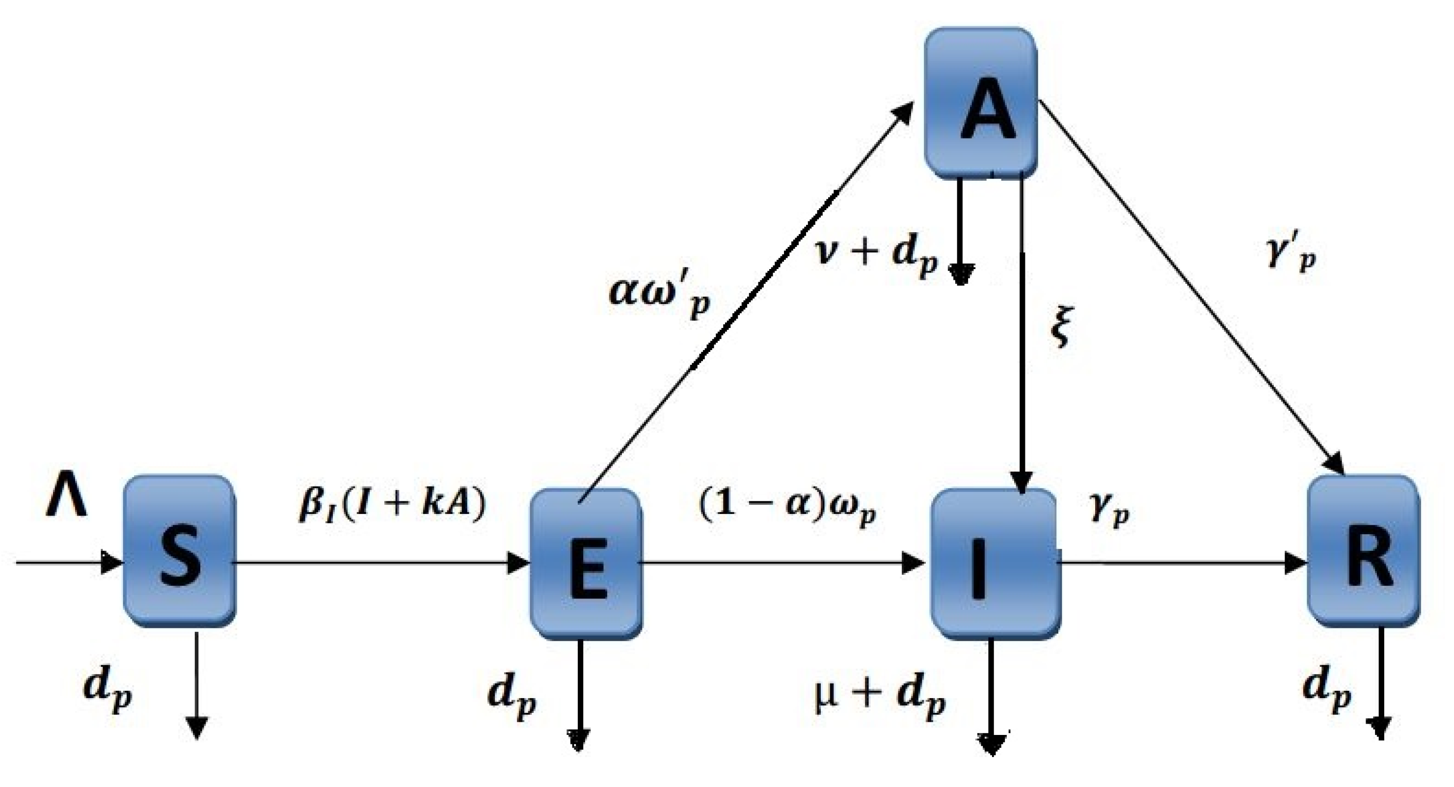
Figure 1. The basic interactions among the compartments.
Fractalfract 05 00087 g001
Figure 2. The model behavior for R 0 = 1.1421 > 1 . (Left) exposed and recovered settle at a level near 2500, susceptibles drop to about 500; (Right) infected stabilize at 120 individuals, asymptomatic instead at 40 individuals. This corresponds to the endemic equilibrium P * . The parameter values are Λ = 500 , β I = 0.01 , k = 0.1 , d p = 0.082 , α = 0.15 , ω p = 0.1 , ω p = 0.1 , ξ = 0.1 , μ = 0.001 , γ p = 1.764 , γ p = 0.6024 , ν = 0.0005 .
Fractalfract 05 00087 g002
Figure 3. The model behavior for 0 < R 0 = 0.0571 < 1 . (Left) susceptibles reach the level of 5500; (Right) infected and asymptomatic individuals are reduced to the single digits, essentially vanishing, recovered and exposed individuals remain confined respectively around the levels 100 and 50. In this situation, the system approaches the disease-free equilibrium P 0 . The parameter values are Λ = 500 , β I = 0.0005 , k = 0.1 , d p = 0.082 , α = 0.15 , ω p = 0.1 , ω p = 0.1 , ξ = 0.1 , μ = 0.001 , γ p = 1.764 , γ p = 0.6024 , ν = 0.0005 .
Fractalfract 05 00087 g003
Figure 4. The model behavior for R 0 = 1.2677 > 1 . (Left) recovered attain the level of 25,000, exposed instead about 4000; (Right) infected stabilize at around the 200 level, susceptibles and asymptomatic individuals remain confined around the level 100. Once again the system settles at the endemic equilibrium, but this time we have ξ = 0 and α = 1 , so that the point attained is P I . The parameter values are Λ = 500 , β I = 0.01 , k = 0.1 , d p = 0.0082 , α = 1 , ω p = 0.1 , ω p = 0.1 , ξ = 0 , μ = 0.001 , γ p = 1.764 , γ p = 0.6024 , ν = 0.0005 .
Fractalfract 05 00087 g004
Figure 5. The model behavior for R 0 = 1.1421 > 1 as q varies in [ 0 , 1 ] . (Left) exposed and recovered; (Right) susceptibles, infected and asymptomatic. The situation corresponds to the endemic equilibrium P * . The parameter values are the same of Figure 2.
Fractalfract 05 00087 g005
Figure 6. The model behavior for 0 < R 0 = 0.0571 < 1 as q varies in [ 0 , 1 ] . (Left) susceptibles; (Right) exposed, infected, asymptomatics and recovered. In this situation the system approaches the disease-free equilibrium P 0 . All the simulations have been stopped at the same final time, T = 10,000. For low values of the fractional derivative order, the populations E, I, A and R are not zero, but this feature is intentionally left in the figure. Thus, it denotes the different speeds at which the populations vanish as a function of the fractional derivative order. The parameter values are the same as those in Figure 3.
Fractalfract 05 00087 g006
Figure 7. The model behavior for R 0 = 1.2677 > 1 as q varies in [ 0 , 1 ] . (Left) exposed and recovered; (Right) susceptibles, infected and asymptomatic. Once again the system settles at the endemic equilibrium, but this time we have ξ = 0 and α = 1 , so that the point attained is P I . The parameter values are the same as those in Figure 4.
Fractalfract 05 00087 g007
Table 1. Model parameters and their meaning.
Λ susceptibles recruitment rate,  
d p natural mortality,  
β I disease transmission rate,  
ktransmissibility ratio between asymptomatics and symptomatics,  
ν disease-related mortality for asymptomatics,  
μ disease-related mortality for symptomatic individuals,  
ω p progression rate from exposed to symptomatic,  
ω p progression rate from exposed to asymptomatic,  
α fraction of exposed that turn asymptomatic,  
ξ progression rate from asymptomatic to symptomatic,  
γ p recovery rate from symptomatic infection,  
γ p recovery rate from asymptomatic infection.  
Publisher’s Note: MDPI stays neutral with regard to jurisdictional claims in published maps and institutional affiliations.