

Exact Traveling Wave Solutions of the Local Fractional Bidirectional Propagation System Equations

1
College of Mathematics and Systems Science, Shandong University of Science and Technology, Qingdao 266590, China
2
School of Mathematics Statistics, Qilu University of Technology (Shandong Academy of Sciences), Jinan 250353, China
*
Author to whom correspondence should be addressed.
Fractal Fract. 2022, 6(11), 653; https://doi.org/10.3390/fractalfract6110653
Submission received: 12 October 2022
/
Revised: 26 October 2022
/
Accepted: 29 October 2022
/
Published: 5 November 2022
(This article belongs to the Special Issue Recent Advances in Computational Physics with Fractional Application)
Abstract
:In this paper, within the scope of the local fractional derivative theory, bidirectional propagation system local fractional equations are researched. Compared with the unidirectional propagation of nonlinear waves in a pipeline, the bidirectional propagation system equations studied in this paper can better describe the propagation of nonlinear waves in a channel. This study is groundbreaking and offers more possibilities for the bidirectional propagation of nonlinear waves in the simulation pipeline. The exact traveling wave solutions of the non-differentiable type defined on the Cantor sets are obtained. The characteristics of the particular solutions of a fixed fractal dimension are discussed. It is proven that the local fractional nonlinear bidirectional wave equations can describe the interaction of fractal waves. It is also shown that the study of traveling wave solutions of nonlinear local fractional equations has important significance in mathematical physics.
1. Introduction
Fractional calculus (FC) has important applications in the physics and engineering fields, such as particle physics [1], wave dynamics [2], electronic systems [3], calculation methods of mathematical physics and so on [4]. The history of fractional derivatives dates back to the 17th century (Diethelm (2010), Oldham and Spanier (1974) and Podlubny (1999)). The concept theory of fractional derivatives is more suitable for modeling. The specific concept of local fractional calculus (LFC) theory was first proposed by Kolwankar and Gangal [5,6,7] based on the Riemann–Liouville fractional order, which is a kind of derivative used to deal with many non-differentiable problems from the perspective of science and engineering [8,9]. When dealing with non-differentiable problems in science and engineering, local models are used to describe fractional ordinary differential equations or partial differential equations. Many media or substances in nature have very complex microstructures, and it is impossible to quantitatively describe their microstructures with simple geometries. Therefore, LFC plays an important role in mathematics, physics and applied science, and its practicability and accuracy are becoming stronger and stronger [10,11].
Recently, there have been many approximation and analytical methods [12] for partial differential equations with local fractional derivative operators, such as the local fractional decomposition method, local fractional variational iteration method, local fractional homotopy perturbation method [13,14] and local fractional class expansion method. At the same time, by applying the local fractional theory and a new effective algorithm [15], the exact solution of the local fractional equation defined on the Cantor set is obtained. Yang [16] redefined and generalized the local order and constructed a complete framework of a local order. A new method for calculating the exact traveling wave solutions of partial-order partial differential equations is proposed, including those of Kortewegdevries [17], Boussinesq [18] and Burgers [19], among others [20]. The results show that the theoretical method is precise, feasible and has great practical significance.
In this paper, we discuss the local fractional equations for a model system describing the bidirectional propagation of nonlinear diffusion waves in water channels as follows. Unlike describing the unidirectional propagation of the nonlinear waves in a pipeline, bidirectional propagation system equations can better describe the propagation of the nonlinear waves in a water channel:
where a, b, c and d are real constants, is the fractal dimension, where x is the distance along the channel (scaled by the undisturbed depth of the water h), and t is the elapsed time scaled by , where g indicates the acceleration of gravity. The variable is the non-dimensional deviation of the water surface (scaled by h), which is from an undisturbed position, and is the non-dimensional horizontal velocity (scaled by ) at a height of the water with above the bottom of the channel [20]. When , Equation (1) is formally equivalent to the classic Boussinesq system, which was derived by Bona, Saut and Toland. It is used to describe a small-amplitude long wave in the waterway, and first-order correction is carried out with a small parameter (representing the typical amplitude depth ratio). The existence of an accurate traveling wave solution is usually very helpful to the theoretical and numerical research of the system.
The main purpose of this paper is to study the exact traveling wave solutions to bidirectional wave equations. This paper is a pioneering study of the local fractional equations for bidirectional propagation systems, providing more possibilities for simulating the bidirectional propagation of nonlinear waves in a pipeline. The structural design of this paper is as follows. In Section 2, the basic theories of the local partial-order derivative (LFD) and local partial-order integral (LFI) are introduced. In Section 3, the exact traveling wave solution of the bidirectional wave equation is given. In Section 4, the special solutions of the bidirectional wave equation with graphs are discussed, and the interactions between the local fractional nonlinear bidirectional wave equations are proven. Finally, the main points are summarized, and the significance and limitations of this study are illustrated in Section 5.
2. Brief of the Local Fractional Derivative
In this section, we introduce the concepts of the local fractional derivative (LFD) and local fractional partial derivatives (LFPDs) of non-differentiable functions, as well as the solutions to local fractional Ricati differential equations (LFRDE):
Definition 1.
Let be a set of non-differentiable functions with a fractal dimension. Assuming that , the local fractional derivative of with an order at the point is defined by [21,22]
where
The special functions defined on the fractal sets are
3. Exact Traveling Wave Solutions of Bidirectional Wave Equations
The focus of this section is to find the exact traveling wave solutions of non-differentiable bidirectional wave equations. First of all, we introduce the local fractional-order bidirectional wave equations:
where is the fractal dimension. In order to find the exact traveling wave solutions of Equation (13), we introduce the complex wave transformations as follows:
where and are constant and
According to the definition and properties of local fractional derivatives, we obtain
By substituting Equation (16) into Equation (13), the local fractional nonlinear ordinary differential equations are given:
Because of the chain rule of the LFD (see M2), Equations (17) and (18) become
where the local fractional derivatives are with respect to . Because we are looking for the solutions of a solitary wave, meaning that the solutions are asymptotically small as they move away from their peaks and thus , as , Equations (19) and (20) can be integrated once to yield
Suppose that and are proportional to each other, namely with B being a constant. We can obtain
For the sake of Equations (23) and (24) having nontrivial solitary wave solutions, the two equations must be the same, which implies
A system of Equations (25) and (26) is linear with respect to the unknowns and , whose solutions depend on the values of and d as follows [27,28,29]:
Case 1: If , then there is only one solution for and to find out.
Case 2: If and , then there are infinitely many solutions, which reads as , where is arbitrary.
Case 3: If and , then there is no solution.
In the case of Equations (25) and (26), by taking the derivative of Equations (23) and (24) and using Equations (25) and (26), we find that this satisfies
The solution to Equation (27) can be obtained by using the following lemma [30], which can be found in many standard works:
Lemma 1.
Let be real constants. The following equation has a solitary wave solution if such that
Moreover, the solitary wave solution can be obtained:
where is an arbitrary constant. Therefore, with the help of the above lemma, Equation (27) is satisfied:
Notice that is not a solution to Equations (25) and (26), so the traveling wave’s exact solution to the bidirectional wave equation is as follows:
The above solutions can be written in a more familiar form. Let
Therefore, the exact traveling wave solution can be expressed as follows:
where , .
4. Discussion of the Solutions
For the convenience of drawing and analysis, we assume that . Then, Equation (34) becomes
When , , then , the Equation(35) is rewritten as
By selecting appropriate parameters, the images of the exact traveling wave solutions of bidirectional wave equations and the interaction with two solitons are drawn as shown in Figure 1 and Figure 2.
It can be seen from Figure 1 that pulse heights of and were within the range of [1.5, 4.5] and [1.5, 4], respectively. Similarly, after the interaction of the two solitons, a pulse height within the range of [1.5, 4.5] was added.
When , , and , the Equation (35) is rewritten as
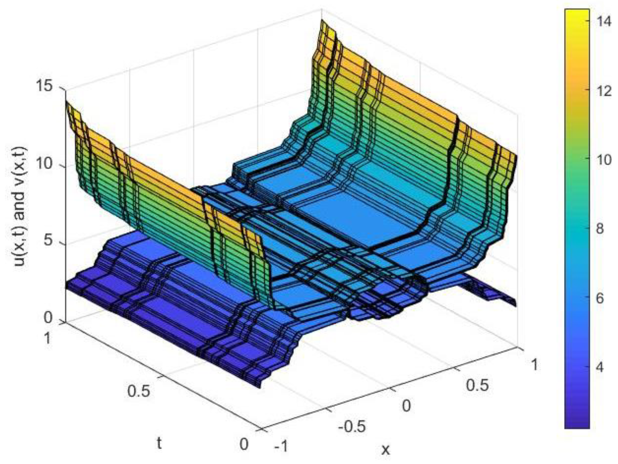
To further investigate the effect of the changing parameters on the exact traveling wave solution of the bidirectional wave equation and the interaction of the two solitons, increasing the velocity parameters, Figure 3 and Figure 4 were obtained.
For the bidirectional wave model, the wave phenomenon described by the local fractional was more accurate, and the numerical simulation results were more suitable for real life.
From Figure 1 and Figure 3, we can clearly see that the bidirectional wave equations can describe fractal waves during the bidirectional propagation of fluid in a waterway. In addition to the physical quantities and forming a pulse, a soliton pulse formed as the time domain expanded. By changing in Equation (33), we obtained Figure 1 and Figure 3. By comparing Figure 1 and Figure 3, it is easy to find that the pulse height of or was higher with the propagation speeds of the waves. In Figure 2 and Figure 4, we show the elastic interaction between two solitons. It can be seen that both solitons maintained their initial velocities and shapes after the interaction. The strength of interaction between the solitons decreased with the increase in soliton spacing.
5. Conclusions
In this study, we first extended the theory of local fractional derivatives and local fractional integrals to a bidirectional propagation system of nonlinear diffusion waves in water channels. We obtained the fractal diagram of the functions with the help of the drawing toolbox in MATLAB (R2019a). The exact traveling 3D figures were given. The propagation process and interaction characteristics of the two solitons described by the bidirectional propagation system were analyzed and discussed. The results show that the characteristic solutions reflected the interaction of fractal waves in nonlinear diffusion waves in waterways. However, there were many practical factors such as the pressure, eddy current and resistance that were not taken into account, and these factors will have an impact on the results, which should be taken into account in the follow-up study. In conclusion, the study of bidirectional propagation system nonlinear local fractional-order equations is of great significance to describing the characteristics of special fractal functions.
Author Contributions
Writing-original draft preparation, X.S.; writing-review and editing, Z.Z.; visualization, H.Y.; supervision, X.H. All authors have read and agreed to the published version of the manuscript.
Funding
This research received no external funding.
Data Availability Statement
Not applicable.
Conflicts of Interest
The authors declare no conflict of interest.
References
- Tarasov, V.E. Fractional Dynamics: Applications of Fractional Calculus to Dynamics of Particles, Fields and Media; Springer Science and Business Mediaew: New York, NY, USA, 2011; pp. 9–10. ISBN 978-3-642-14002-0. [Google Scholar]
- Momani, S.; Odibat, Z.; Alawneh, Z. Variational iteration method for solving the spaceand time-fractional KdV equation. Numer. Methods Partial. Differ. Equ. Int. J. 2008, 24, 262–271. [Google Scholar] [CrossRef]
- West, B.; Bologna, M.; Grigolini, P. Physics of fractal operators. In Institute for Nonlinear Science; Springer: New York, NY, USA, 2003; pp. 34–40. ISBN 978-0-387-21746-8. [Google Scholar]
- Mohyud-Din, S.T.; Yıldırım, A.; Yülüklü, E. Homotopy analysis method for space-and time-fractional KdV equation. Int. J. Numer. Methods Heat Fluid Flow 2012, 22, 928–941. [Google Scholar] [CrossRef]
- Yang, X.J. Advanced Local Fractional Calculus and Its Applications; World Science: New York, NY, USA, 2012; pp. 29–30. ISBN 978-1-938576-01-0. [Google Scholar]
- Kolwankar, K.M.; Gangal, A.D. Fractional differentiability of nowhere differentiable functions and dimensions. Chaos 1996, 6, 505–513. [Google Scholar] [CrossRef] [PubMed] [Green Version]
- Kilbas, A.A.; Srivastava, H.M.; Trujillo, J.J. Theory and Applications of Fractionaldifferential Equations North-Holland Mathematical Studies; Elsevier (North-Holland) Science Publishers: Amsterdam, The Netherlands; London, UK; New York, NY, USA, 2006; Volume 204. [Google Scholar]
- Wang, K.L.; Wang, K.J.; He, C.H. Physical insight of local fractional calculus and its application to fractional KdV-Burgers-Kuramoto equation. Fractals 2019, 27, 1950122. [Google Scholar] [CrossRef]
- Iftikhar, S.; Kumam, P.; Erden, S. Newton’s-type integral inequalities via local fractiona integrals. Fractals 2020, 28, 20500372. [Google Scholar] [CrossRef]
- Yong, Z. Basic Theory of Fractional Differential Equations; World Scientific: Singapore, 2014; pp. 19–25. ISBN 978-8-813148-16-1. [Google Scholar]
- Matignon, D. Stability results for fractional differential equations with applications to control processing. Comput. Eng. Syst. Appl. 1996, 2, 963–968. [Google Scholar]
- Adomian, G. A review of the decomposition method and some recent results for nonlinear equations. J. Appl. Math. Comput. 1991, 21, 101–127. [Google Scholar] [CrossRef] [Green Version]
- Liao, S. On the homotopy analysis method for nonlinear problems. J. Appl. Math. Comput. 2004, 147, 499–513. [Google Scholar] [CrossRef]
- Odibat, Z.; Sami Bataineh, A. An adaptation of homotopy analysis method for reliable treatment of strongly nonlinear problems: Construction of homotopy polynomials. Math. Methods Appl. Sci. 2015, 38, 991–1000. [Google Scholar] [CrossRef]
- Singh, J.; Ahmadian, A.; Rathore, S. An efficient computational approach for local fractional Poisson equation in fractal media. Numer. Methods Partial. Differ. Equ. 2020, 37, 1439–1448. [Google Scholar] [CrossRef]
- Yang, X.J.; Baleanu, D.; Srivastava, H.M. Local Fractional Integral Transforms and Their Applications; Academic Press: Cambridge, MA, USA, 2015; pp. 39–50. ISBN 978-0-12-804002-7. [Google Scholar]
- Gao, F.; Yang, X.J.; Ju, Y. Exact traveling-wave solutions for one-dimensional modified Korteweg-de Vries equation defined on Cantor sets. Fractals 2019, 27, 1940010. [Google Scholar] [CrossRef]
- Yang, X.J.; Machado, J.T.; Baleanu, D. Exact traveling-wave solution for local fractional Boussinesq equation in fractal domain. Fractals 2017, 25, 1740006. [Google Scholar] [CrossRef] [Green Version]
- Yang, X.J.; Gao, F.; Srivastava, H.M. Exact travelling wave solutions for the local fractional two-dimensional Burgers-type equations. Comput. Math. Appl. 2017, 73, 203–210. [Google Scholar] [CrossRef]
- Yang, X.J.; Machado, J.T.; Baleanu, D.; Cattani, C. On exact traveling-wave solutions for local fractional Korteweg-de Vries equation. Chaos Interdiscip. J. Nonlinear Sci. 2016, 26, 084312. [Google Scholar] [CrossRef]
- Chen, M. Exact traveling-wave solutions to bidirectional wave equations. Int. J. Theor. Phys. 1998, 37, 1547–1567. [Google Scholar] [CrossRef]
- Gorenflo, R.; Mainardi, F. Fractional Calculus: Integral and Differential Equations of Fractional Order. Mathematics 2008, 49, 277–290. [Google Scholar]
- Krni, M.; Vukovi, P. Multidimensional Hilbert-Type Inequalities Obtained via Local Fractional Calculus. Acta Appl. Math. 2020, 169, 667–680. [Google Scholar] [CrossRef]
- Yang, X.J.; Gao, F.; Srivastava, H.M. Non-differentiable exact solutions for the nonlinear odes defined on fractal sets. Fractals 2017, 25, 1740002. [Google Scholar] [CrossRef] [Green Version]
- Yang, X.J.; Srivastava, H.M.; Torres, D.F.M.; Zhang, Y.D. Non-differentiable solutions for local fractional nonlinear Riccati differential equations. Fund. Inform. 2016, 145, 55–63. [Google Scholar] [CrossRef] [Green Version]
- Yang, X.J.; Gao, F.; Srivastava, H.M. New rheological models within local fractional derivative. Rom. Rep. Phys. 2017, 69, 113. [Google Scholar]
- Bona, J.L.; Saut, J.C.; Toland, J.F. Boussinesq equations for small-amplitude long wavelength water waves. Preprint 1997. [Google Scholar]
- Bona, J.L.; Smith, R. A model for the two-way propagation of water waves in a channel. MAthematical Proc. Camb. Philos. Soc. 1976, 79, 167–182. [Google Scholar] [CrossRef]
- Boussinesq, J. TheÂorie de l’intumescence liquide appeleÂe onde solitaire ou de translationse propageant dans un canal rectangulaire. Comptes Rendus L’Acadmie Sci. 1871, 72, 755–759. [Google Scholar]
- Newell, A.C. Finite amplitude instabilities of partial difference equations. SIAM J. Appl. Math. 1977, 33, 133–160. [Google Scholar] [CrossRef]
Figure 1.
Exact traveling wave solutions of bidirectional wave equations with and .
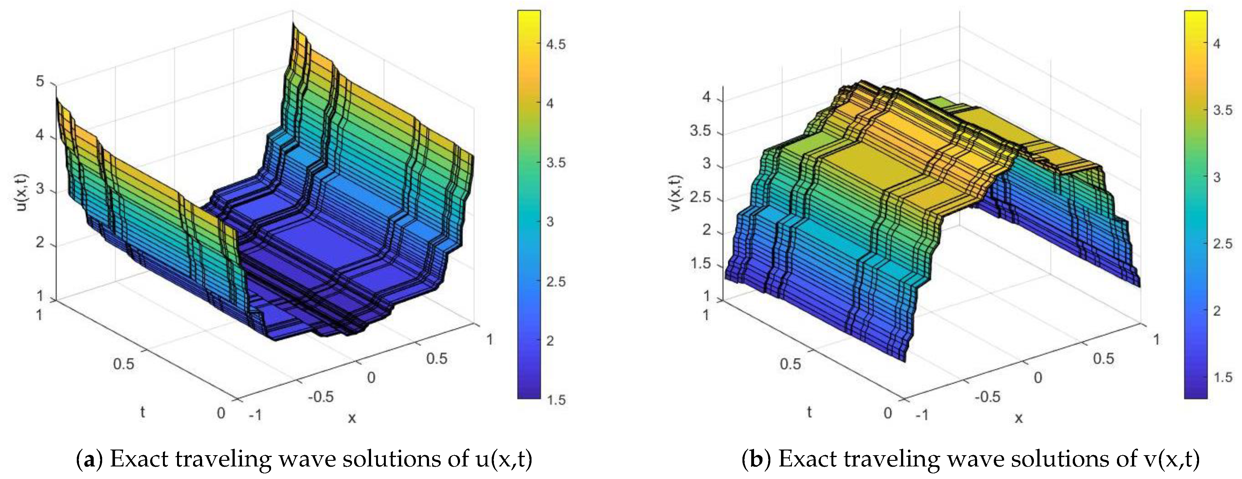
Figure 2.
The interaction with two solitons, with and .

Figure 3.
Exact traveling wave solutions of bidirectional wave equations with and .
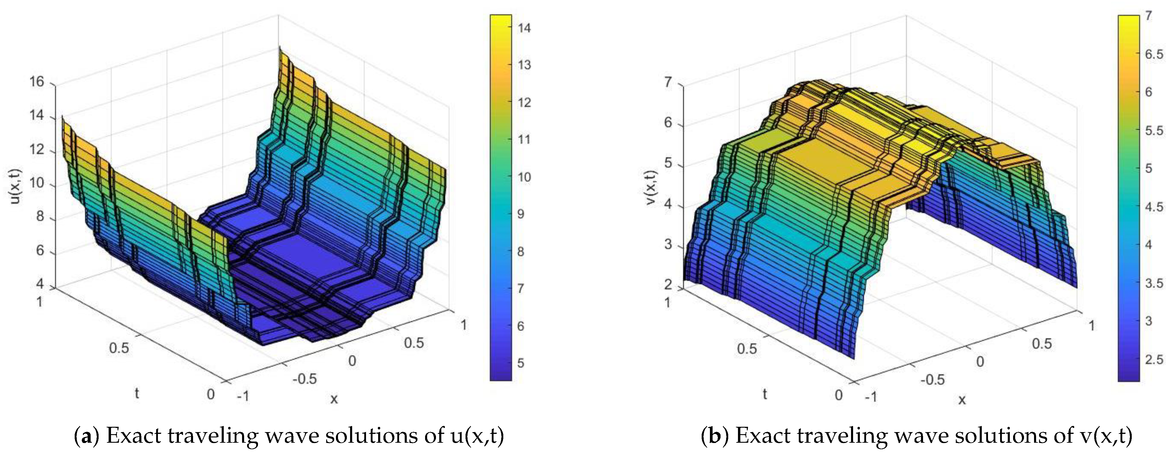
Figure 4.
The interaction with two solitons, with and .
Publisher’s Note: MDPI stays neutral with regard to jurisdictional claims in published maps and institutional affiliations. |
© 2022 by the authors. Licensee MDPI, Basel, Switzerland. This article is an open access article distributed under the terms and conditions of the Creative Commons Attribution (CC BY) license (https://creativecommons.org/licenses/by/4.0/).
Share and Cite
MDPI and ACS Style
Sang, X.; Zhang, Z.; Yang, H.; Han, X. Exact Traveling Wave Solutions of the Local Fractional Bidirectional Propagation System Equations. Fractal Fract. 2022, 6, 653. https://doi.org/10.3390/fractalfract6110653
AMA Style
Sang X, Zhang Z, Yang H, Han X. Exact Traveling Wave Solutions of the Local Fractional Bidirectional Propagation System Equations. Fractal and Fractional. 2022; 6(11):653. https://doi.org/10.3390/fractalfract6110653
Chicago/Turabian StyleSang, Xue, Zongguo Zhang, Hongwei Yang, and Xiaofeng Han. 2022. "Exact Traveling Wave Solutions of the Local Fractional Bidirectional Propagation System Equations" Fractal and Fractional 6, no. 11: 653. https://doi.org/10.3390/fractalfract6110653