A Reliable Approach for Solving Delay Fractional Differential Equations

Abstract

In this paper, we study a class of second-order delay fractional differential equations with a variable-order Caputo derivative. This type of equation is an extension to ordinary delay equations which are used in the modeling of several biological systems such as population dynamics, epidemiology, and immunology. Usually, fractional differential equations are difficult to solve analytically, and with fractional derivatives of variable-order, they become more challenging. Therefore, the need for reliable numerical techniques is worth investigating. To solve this type of equation, we derive a new approach based on the operational matrix. We use the shifted Chebyshev polynomials of the second kind as the basis for the approximate solutions. A convergence analysis is discussed and the uniform convergence of the approximate solutions is proven. Several examples are discussed to illustrate the efficiency of the presented approach. The computed errors, figures, and tables show that the approximate solutions converge to the exact ones by considering only a few terms in the expansion, and illustrate the novelty of the presented approach.

1. Introduction

Fractional differential equations (FDEs) appear in several science and engineering applications. They have been used to model several nonlocal dynamical systems [1,2] and, thus, have become a popular field of study. Fractional delay differential equations (FDDEs) are also emerging in many other disciplines, including chemistry, physics, and finance, where the inclusion of the delay term in the differential equations opens new vistas [3]. Because it is extremely difficult to obtain solutions of nonlinear FDEs and FDDEs in closed forms, several analytical and numerical methods such as the Adomian decomposition and homotopy perturbations methods have been implemented [4,5,6,7,8,9,10,11,12,13]. In [14,15], authors derived numerical approaches for the numerical integration of FDEs, which are a generalization of many known methods in the literature, such as the Adams–Bashforth approach. Adams–Bashforth methods were implemented to solve nonlinear FDDEs [16,17]. In addition, Daftardar-Gejji et al. recently introduced the predictor–corrector method for solving FDEs [18]. A new iterative method to numerically solve FDEs was derived in [19] and implemented for various functional equations. The operational matrix method (OMM) has been proven to be an efficient approach to approximate various functional equations. Gurbuz and Mehmet [20,21,22,23] implemented the OMM based on the Laguerre polynomials to solve several types of linear and nonlinear functional equations, including the mixed boundary condition. Recently, the OMM was used by several researchers to solve fractional differential equations. It was implemented to solve the fractional Riccati equations [24], the generalized Abel integral equations [25], and fractional differential equations of arbitrary order [26].

In this article, we study the following fractional delay problem:

$$\begin{array}{c}{D}^{2}z\left(s\right)=D^{\mu \left(s\right)}z\left(s\right)+a\left(s\right)z\left(\zeta s\right)+r\left(s\right),0<s<1,\end{array}$$

(1)

$$\begin{array}{c}z\left(0\right)=z_0,z^{\prime }\left(0\right)=z_1,\hspace{1em}\hspace{1em}\hspace{1em}\hspace{1em}\hspace{1em}\hspace{1em}\hspace{1em}\hspace{1em}\hfill \end{array}$$

(2)

where $0<\zeta <1$, $0<\mu \left(s\right)<1$ for all $s\in [0,1]$, $a\left(s\right),r\left(s\right)$ are a continuous function on $[0,1]$, and $D^{\mu \left(s\right)}$ is the variable Caputo derivative. In the next section, we present some definitions and formulas which are used later. The method of solution is discussed in Section 3, and in Section 4, we present some theoretical results. Several examples are discussed in Section 5. In addition, we present conclusions in the last section.

2. Basic Definitions and Formulas

Here, we focused on basic concepts and definitions which were used in this paper. We started with the definition of the variable Caputo derivative.

Definition 1. 

Let$\mu :[0,1]\to (0,1)$be a real valued function, and$u\in AC[0,1].$The Caputo derivative of variable fractional order μ is defined by

$$D^{\mu \left(x\right)}u\left(x\right)=\frac{1}{\mathrm{\Gamma }(1-\mu (x\left)\right)}{\int }_0^x\frac{u^{\prime }\left(x\right)}{{(x-s)}^{\mu \left(x\right)}}ds.$$

(3)

Then, the following formulas can be obtained:

$$D^{\mu \left(x\right)}{x}^m=\frac{\mathrm{\Gamma }(m+1)}{\mathrm{\Gamma }(1+m-\mu (x\left)\right)}{x}^{m-\mu \left(x\right)},m=1,2,...$$

(4)

and

$$D^{\mu \left(x\right)}1=0.$$

(5)

For more details about the definition and properties of the variable Caputo derivatives, we refer the reader to [27,28,29]. Let ${\left\{T_k\left(x\right)\right\}}_{k=0}^{\infty }$ be the set of Chebyshev polynomials of the second kind on $[-1,1]$. Then,

$${\int }_{-1}^1\omega \left(x\right)T_k\left(x\right)T_l\left(x\right)dx=\left\{\begin{array}{cc}\frac{\pi }{2},\hfill & k=l\hfill \\ 0,\hfill & k\ne l\hfill \end{array}\right.$$

(6)

where $\omega \left(x\right)=\sqrt{1-x^2}$. The relation that generates these polynomials is given by

$$T_{k+1}\left(x\right)=2x{T}_k\left(x\right)-T_{k-1}\left(x\right),k=1,2,...$$

(7)

where

$$\begin{array}{ccc}& & T_0\left(x\right)=1,\hfill \end{array}$$

(8)

$$\begin{array}{ccc}& & T_1\left(x\right)=2x.\hfill \end{array}$$

(9)

Let $x=2s-1$. We defined the polynomials $S{T}_k\left(s\right)$ by

$$S{T}_k\left(s\right)=T_k(2s-1),k=0,1,.\dots$$

(10)

Then, it held that

$$S{T}_{k+1}\left(s\right)=(4s-2)S{T}_k\left(s\right)-S{T}_{k-1}\left(s\right),k=1,2,\dots$$

(11)

where

$$\begin{array}{c}S{T}_0\left(s\right)=1,\hspace{1em}\hspace{1em}\hfill \end{array}$$

(12)

$$\begin{array}{c}S{T}_1\left(s\right)=4s-2.\hfill \end{array}$$

(13)

Then, simple calculations indicate that $S{T}_2\left(s\right)$ and $S{T}_3\left(s\right)$ are given by

$$\begin{array}{c}S{T}_2\left(s\right)=(4s-2)S{T}_1\left(s\right)-S{T}_0\left(s\right)=16s^2-16s+3,\hspace{1em}\hspace{1em}\hfill \end{array}$$

(14)

$$\begin{array}{c}S{T}_3\left(s\right)=(4s-2)S{T}_2\left(s\right)-S{T}_1\left(s\right)=64s^3-96s^2-24s-4.\hfill \end{array}$$

(15)

Thus, the coefficient of the leading term in $S{T}_k\left(S\right)$ is $4^k$. The orthogonality relation is given as

$${\int }_0^{1}s\omega \left(s\right)S{T}_k\left(s\right)S{T}_l\left(s\right)ds=\left\{\begin{array}{cc}\frac{\pi }{8},\hfill & k=l\hfill \\ 0,\hfill & k\ne l\hfill \end{array}\right.$$

(16)

where $s\omega \left(s\right)=\sqrt{s-s^2}$. One can see that if $f\left(s\right)$ is a smooth function on $[0,1]$, then it can be written in terms of $\{S{T}_k\left(s\right),k=0,1,2,\dots \}$ as follows:

$$f\left(s\right)=\sum _{k=0}^{\infty }{a}_{k}S{T}_k\left(s\right)$$

(17)

where

$$a_k=\frac{8}{\pi }{\int }_0^{1}s\omega \left(s\right)S{T}_k\left(s\right)f\left(s\right)ds.$$

(18)

Now, we could find a relation between the basis $\{1,s,\dots ,s^m\}$ and the basis $\{S{T}_0\left(s\right),S{T}_1\left(s\right),\dots ,S{T}_m\left(s\right)\}$. Let ${\mathrm{Y}}_m\left(s\right)={\left[S{T}_0\left(s\right),S{T}_1\left(s\right),\dots ,S{T}_m\left(s\right)\right]}^T$ and ${\mathrm{\Phi }}_m\left(s\right)=$${\left[1,s,\dots ,s^m\right]}^T$. Then,

$${\mathrm{Y}}_m\left(s\right)=A_m{\mathrm{\Phi }}_m\left(s\right)$$

(19)

where for $m=5$

$$A_5=\left(\begin{array}{ccccc}1& 0& 0& 0& 0\\ -2& 2^2& 0& 0& 0\\ 3& -16& 2^4& 0& 0\\ -4& 40& -96& 2^6& 0\\ 5& -80& 336& -512& 2^8\end{array}\right).$$

(20)

It is easy to see that $A_m$ is a lower triangular matrix with the following diagonal elements

$${\left(A_m\right)}_{kk}=2^{2k-2}.$$

(21)

We had $det\left(A_m\right)=2^{m^2-m}\ne 0$, which implies that $A_m$ is a nonsingular matrix and it held that

$${\mathrm{\Phi }}_m\left(s\right)=A_m^{-1}{\mathrm{Y}}_m\left(s\right).$$

(22)

3. Method of Solution

This section focuses on the derivation of the proposed method. First, we found the operational matrices of $D^{2}z\left(s\right),z\left(\zeta s\right)$, and $D^{\mu \left(s\right)}z\left(s\right)$. From Equation (19), we had

$$\begin{array}{ccc}\hfill {\mathrm{Y}}_m^{″}\left(s\right)& =& \frac{d^2}{d{s}^2}\left[A_m{\mathrm{\Phi }}_m\left(s\right)\right]=A_m\frac{d^2}{d{s}^2}{\mathrm{\Phi }}_m\left(s\right)\hfill \end{array}$$

(23)

$$\begin{array}{ccc}& =& A_m\left(\begin{array}{c}0\\ 0\\ 2\\ ⋮\\ m(m-1)s^{m-2}\end{array}\right)\hfill \\ \hfill & =& A_m{F}_m{\mathrm{\Phi }}_m\left(s\right)\hfill \\ \hfill & =& A_m{F}_m{A}_m^{-1}{\mathrm{Y}}_m\left(s\right),\hfill \end{array}$$

(24)

where

$$F_m=\left(\begin{array}{ccccccc}0& 0& 0& \cdots & 0& 0& 0\\ 0& 0& 0& \cdots & 0& 0& 0\\ 2& 0& 0& \cdots & 0& 0& 0\\ 0& 6& 0& \cdots & 0& 0& 0\\ ⋮& ⋮& ⋮& ⋮& ⋮& ⋮& ⋮\\ 0& 0& 0& \cdots & m(m-1)& 0& 0\end{array}\right).$$

(25)

Hence, $A_m{F}_m{A}_m^{-1}$ was the operational matrix of ${\mathrm{Y}}_m^{″}\left(s\right)$. Now,

$$\begin{array}{ccc}{\mathrm{Y}}_m\left(\zeta s\right)& =& A_m{\mathrm{\Phi }}_m\left(\zeta s\right)\end{array}$$

(26)

$$\begin{array}{c}\hfill \hspace{1em}\hspace{1em}\hspace{1em}\hspace{1em}=A_m\left(\begin{array}{c}1\\ \zeta s\\ {\zeta }^2{s}^2\\ ⋮\\ {\zeta }^m{s}^m\end{array}\right)\\ \hfill \hspace{1em}\hspace{1em}\hspace{1em}\hspace{1em}=A_m{G}_m{\mathrm{\Phi }}_m\left(s\right),\end{array}$$

(27)

where

$$G_m=\left(\begin{array}{ccccc}1& 0& 0& ·& 0\\ 0& \zeta & 0& \cdots & 0\\ ⋮& ⋮& ⋮& ⋮& ⋮\\ 0& 0& \cdots & {\zeta }^{m-1}& 0\\ 0& 0& \cdots & 0& {\zeta }^m\end{array}\right).$$

(28)

From Equation (26), we obtained

$${\mathrm{Y}}_m\left(\zeta s\right)=A_m{G}_m{A}_m^{-1}{\mathrm{Y}}_m\left(s\right).$$

(29)

Hence, $A_m{G}_m{A}_m^{-1}$ was the operational matrix of ${\mathrm{Y}}_m\left(\zeta s\right)$. Finally,

$$\begin{array}{c}{D}^{\mu \left(s\right)}{\mathrm{Y}}_m\left(s\right)=D^{\mu \left(s\right)}\left(A_m{\mathrm{\Phi }}_m\left(s\right)\right)\hfill \end{array}$$

(30)

$$\begin{array}{c}\hspace{1em}\hspace{1em}\hspace{1em}\hspace{1em}=A_m\left(\begin{array}{c}{D}^{\mu \left(s\right)}1\\ D^{\mu \left(s\right)}s\\ ⋮\\ D^{\mu \left(s\right)}{s}^m\end{array}\right)\\ \hspace{1em}\hspace{1em}\hspace{1em}\hspace{1em}\hspace{1em}\hspace{1em}=A_m\left(\begin{array}{c}0\\ \frac{\mathrm{\Gamma }\left(2\right)}{\mathrm{\Gamma }(2-\mu (s\left)\right)}{s}^{1-\mu \left(s\right)}\\ ⋮\\ \frac{\mathrm{\Gamma }(m+1)}{\mathrm{\Gamma }(m+1-\mu (s\left)\right)}{s}^{m-\mu \left(s\right)}\end{array}\right)\\ \hspace{1em}\hspace{1em}\hspace{1em}\hspace{1em}\hspace{1em}\hspace{1em}\hspace{1em}\hspace{1em}\hspace{1em}\hspace{1em}\hspace{1em}\hspace{1em}\hspace{1em}=A_m\left(\begin{array}{cccc}0& 0& \cdots & 0\\ 0& \frac{\mathrm{\Gamma }\left(2\right)}{\mathrm{\Gamma }(2-\mu (s\left)\right)}{s}^{-\mu \left(s\right)}& \cdots & 0\\ ⋮& ⋮& ⋮& \cdots \\ 0& 0& \cdots & \frac{\mathrm{\Gamma }(m+1)}{\mathrm{\Gamma }(m+1-\mu (s\left)\right)}{s}^{-\mu \left(s\right)}\end{array}\right){\mathrm{\Phi }}_m\left(s\right)\\ =A_m{N}_{\mu \left(s\right)}{A}_m^{-1}{\mathrm{Y}}_m\left(s\right)\end{array}$$

(31)

where

$$N_{\mu \left(s\right)}=\left(\begin{array}{cccc}0& 0& \cdots & 0\\ 0& \frac{\mathrm{\Gamma }\left(2\right)}{\mathrm{\Gamma }(2-\mu (s\left)\right)}{s}^{-\mu \left(s\right)}& \cdots & 0\\ ⋮& ⋮& ⋮& \cdots \\ 0& 0& \cdots & \frac{\mathrm{\Gamma }(m+1)}{\mathrm{\Gamma }(m+1-\mu (s\left)\right)}{s}^{-\mu \left(s\right)}\end{array}\right).$$

(32)

Hence, $A_m{N}_{\mu \left(s\right)}{A}_m^{-1}$ was the operational matrix of $D^{\mu \left(s\right)}{\mathrm{Y}}_m\left(s\right)$. Let

$$Z_m\left(s\right)=\sum _{k=0}^m{\nu }_{k}S{T}_k\left(s\right)={\mathrm{\Theta }}_m{\mathrm{Y}}_m\left(s\right)$$

(33)

where

$${\mathrm{\Theta }}_m=\left(\begin{array}{ccccc}{\nu }_0& {\nu }_1& {\nu }_2& \cdots & {\nu }_m\end{array}\right).$$

(34)

From Equations (1), (23), (29) and (30), we obtained

$${\mathrm{\Theta }}_m\left(A_m{F}_m{A}_m^{-1}\right){\mathrm{Y}}_m\left(s\right)={\mathrm{\Theta }}_m(A_m{N}_{\mu \left(s\right)}{A}_m^{-1}+a\left(s\right)A_m{G}_m{A}_m^{-1}){\mathrm{Y}}_m\left(s\right)+r\left(s\right)$$

(35)

or

$${\mathrm{\Theta }}_m(A_m{F}_m{A}_m^{-1}-A_m{N}_{\mu \left(s\right)}{A}_m^{-1}-a\left(s\right)A_m{G}_m{A}_m^{-1}){\mathrm{Y}}_m\left(s\right)=r\left(s\right).$$

(36)

Taking the collocation points

$$s_k=\frac{2k+2}{2m+2},k=1,2,\dots ,m-1,$$

(37)

we had

$${\mathrm{\Theta }}_m(A_m{F}_m{A}_m^{-1}-A_m{N}_{\mu \left(s_k\right)}{A}_m^{-1}-a\left(s_k\right)A_m{G}_m{A}_m^{-1}){\mathrm{Y}}_m\left(s_k\right)=r\left(s_k\right),k=1,2,\dots ,m-1.$$

(38)

Now, From Equation (33), we had

$$\begin{array}{c}{z}_0=Z_m\left(0\right)={\mathrm{\Theta }}_m{\mathrm{Y}}_m\left(0\right),\hspace{1em}\hspace{1em}\hspace{1em}\hfill \end{array}$$

(39)

$$\begin{array}{c}{z}_1=Z_m^{\prime }\left(0\right)=A_m{N}_{\mu \left(1\right)}{A}_m^{-1}{\mathrm{Y}}_m\left(0\right),\hfill \end{array}$$

(40)

which, combined with the results in Equations (38)–(40), led to

$$\prod \left({\mathrm{\Theta }}_m\right)=\mathrm{\Psi },$$

(41)

where

$$\prod \left({\mathrm{\Theta }}_m\right)=\left(\begin{array}{c}{\mathrm{\Theta }}_m(A_m{F}_m{A}_m^{-1}-A_m{N}_{\mu \left(s_1\right)}{A}_m^{-1}-a\left(s_1\right)A_m{G}_m{A}_m^{-1}){\mathrm{Y}}_m\left(s_1\right)\\ {\mathrm{\Theta }}_m(A_m{F}_m{A}_m^{-1}-A_m{N}_{\mu \left(s_2\right)}{A}_m^{-1}-a\left(s_2\right)A_m{G}_m{A}_m^{-1}){\mathrm{Y}}_m\left(s_2\right)\\ ⋮\\ {\mathrm{\Theta }}_m(A_m{F}_m{A}_m^{-1}-A_m{N}_{\mu \left(s_{m-1}\right)}{A}_m^{-1}-a\left(s_{m-1}\right)A_m{G}_m{A}_m^{-1}){\mathrm{Y}}_m\left(s_{m-1}\right)\\ {\mathrm{\Theta }}_m{\mathrm{Y}}_m\left(0\right)\\ A_m{N}_{\mu \left(1\right)}{A}_m^{-1}{\mathrm{Y}}_m\left(0\right)\end{array}\right),\mathrm{\Psi }=\left(\begin{array}{c}r\left(s_1\right)\\ r\left(s_2\right)\\ ⋮\\ r\left(s_{m-1}\right)\\ z_0\\ z_1\end{array}\right).$$

(42)

Then, we solve the nonlinear algebraic system (41) using Wolfram Research, Inc., Mathematica, Version 12.1, Champaign, IL (2021), to find ${\mathrm{\Theta }}_m$.

4. Theoretical Results

Our main task in this section was to show that $\{Z_m\left(s\right):m=1,2,\dots \}$ converged uniformly to $z\left(s\right)$ on $[0,1]$. Since the differential operator on the Chebyshev polynomials space was continuous and bounded, see [30], the solution produced by the operational matrix method was very close to the least squares approximation of $z\left(s\right)$. For simplicity in analyzing the method, we assumed that $z_m\left(s\right)$ was the least square approximation of $z\left(s\right)$. Let $z\left(s\right)\in C^{m+1}[0,1]$, and assume that

$$Z_m\left(s\right)=\sum _{k=0}^m{\nu }_{k}S{T}_k\left(s\right)={\mathrm{\Theta }}_m{\mathrm{Y}}_m\left(s\right)$$

(43)

was the least square approximation of $z\left(s\right)$ of degree m. Using Taylor’s series expansion, we had

$$z\left(s\right)={\sigma }_m\left(s\right)+\frac{z^{m+1}\left(\alpha \right){(s-c)}^{m+1}}{(m+1)!},$$

(44)

where $c\in [0,1]$, $\alpha$ between s and c, and

$${\sigma }_m\left(s\right)=\sum _{k=0}^m\frac{z^{\left(k\right)}\left(c\right){(s-c)}^k}{k!}.$$

(45)

Thus,

$$|z\left(s\right)-{\sigma }_m\left(s\right)|=\left|\frac{z^{m+1}\left(\alpha \right){(s-c)}^{m+1}}{(m+1)!}\right|.$$

(46)

Since $Z_m\left(s\right)$ was the least squares approximation of $z\left(s\right)$, we had

$$\begin{array}{c}\parallel z-Z_m{\parallel }_2^2\le \parallel z-{\sigma }_m{\parallel }_2^2\hspace{1em}\hspace{1em}\hspace{1em}\hspace{1em}\hspace{1em}\hspace{1em}\hspace{1em}\hspace{1em}\hspace{1em}\hspace{1em}\hfill \end{array}$$

(47)

$$\begin{array}{c}={\int }_0^{1}s\omega \left(x\right){(z\left(s\right)-\sigma \left(s\right))}^{2}ds\hfill \end{array}$$

(48)

$$\begin{array}{c}={\int }_0^{1}s\omega \left(s\right)\frac{z^{m+1}\left(\alpha \right){(s-c)}^{m+1}}{{((m+1)!)}^2}ds\hfill \end{array}$$

(49)

$$\begin{array}{c}\le \frac{{\tau }^2}{{((m+1)!)}^2}{\int }_0^{1}s\omega \left(x\right){(s-c)}^{2m+2}ds\hfill \end{array}$$

(50)

$$\begin{array}{c}=\frac{{\tau }^2}{{((m+1)!)}^2}{\int }_0^1\sqrt{s-s^2}{(s-c)}^{2m+2}dx,\hfill \end{array}$$

(51)

where

$$\tau =max\{z^{(m+1)}\left(s\right):s\in [0,1]\}.$$

(52)

Let $\gamma =max\{1-c,c\}$. Then,

$$\parallel z-Z_m{\parallel }_2^2\le \frac{{\tau }^2{\gamma }^{2m+2}}{{((m+1)!)}^2}{\int }_0^1\sqrt{s+s^2}=\frac{{\tau }^2{\gamma }^{2m+2}}{{((m+1)!)}^2}\frac{\pi }{8}.$$

(53)

Therefore,

$$\parallel z-Z_m{\parallel }_2\le \frac{\tau {\gamma }^{m+}}{(m+1)!}\sqrt{\frac{\pi }{8}},$$

(54)

which approached to zero as m approached to ∞ for all $s\in [0,1]$. Thus, $\{Z_m\left(s\right):m=1,2,\dots \}$ converged uniformly to $z\left(s\right)$ on $[0,1]$. The previous discussion was proof of the following theorem:

Theorem 1. 

Suppose that$z\left(s\right)\in C^{m+1}[0,1]$. Let$Z_m\left(s\right)={\sum }_{k=0}^m{\nu }_{k}S{T}_k\left(s\right)={\mathrm{\Theta }}_m{\mathrm{Y}}_m\left(s\right)$be the least squares approximation of$z\left(s\right)$. Then,$\{Z_m\left(s\right):m=1,2,\dots \}$converges uniformly to$z\left(s\right)$on$[0,1]$.

5. Examples

Three numerical examples were solved to show the efficiency of the OMM.

Example 1. 

Consider the delay fractional problem

$$\begin{array}{c}{D}^{2}z\left(s\right)=D^{\frac{3sins+2coss}{10}}z\left(s\right)+sz\left(\frac{s}{2}\right)+r\left(s\right),0<s<1\hfill \end{array}$$

(55)

$$\begin{array}{c}z\left(0\right)=0,z^{\prime }\left(0\right)=1,\hspace{1em}\hspace{1em}\hspace{1em}\hspace{1em}\hspace{1em}\hspace{1em}\hspace{1em}\hspace{1em}\hspace{1em}\hspace{1em}\hspace{1em}\hfill \end{array}$$

(56)

where

$$r\left(s\right)=2-\frac{2}{\mathrm{\Gamma }(3-\frac{3sins+2coss}{10})}{s}^{2-\frac{3sins+2coss}{10}}-\frac{1}{\mathrm{\Gamma }(2-\frac{3sins+2coss}{10})}{s}^{1-\frac{3sins+2coss}{10}}-\frac{s^3}{4}-\frac{s^2}{2}.$$

(57)

The exact solution was given by

$$z\left(s\right)=s^2+s.$$

(58)

Let the approximate solution be given by

$$Z_5\left(s\right)=\sum _{k=0}^5{\nu }_{k}S{T}_k\left(s\right).$$

(59)

Then, using the proposed method, we obtained

$${\nu }_0=0.8125000000000001,{\nu }_1=0.5,{\nu }_2=0.0625,{\nu }_3={\nu }_4={\nu }_5=0.$$

(60)

Thus,

$$Z_5\left(s\right)=0.8125000000000001S{T}_0\left(s\right)+0.5S{T}_1\left(s\right)+0.0625S{T}_2\left(s\right)=1.11022\times {10}^{-16}+s+s^2.$$

(61)

Let

$${ϵ}_5=max\left\{\right|z\left(0\right)-Z_5\left(0\right)|,|z\left(s_1\right)-Z_5\left(s_1\right)|,\dots ,|z\left(s_4\right)-Z_5\left(s_4\right)|,|z\left(1\right)-Z_5\left(1\right)\left|\right\}.$$

(62)

Then,${ϵ}_5=1.11022\times {10}^{-16}$. The absolute errors are reported in Table 1. The graphs of$z\left(s\right)$and$Z_5\left(s\right)$are shown in Figure 1.

Table 1. Absolute error for Example 1.

s	$|\mathit{z}\left(\mathit{s}\right)-{\mathit{Z}}_5\left(\mathit{s}\right)|$
0	$1.11022\times {10}^{-16}$
0.1	$1.11022\times {10}^{-16}$
0.2	$1.11022\times {10}^{-16}$
0.3	$1.11022\times {10}^{-16}$
0.4	$1.11022\times {10}^{-16}$
0.5	$1.11022\times {10}^{-16}$
0.6	$1.11022\times {10}^{-16}$
0.7	$1.11022\times {10}^{-16}$
0.8	$1.11022\times {10}^{-16}$
0.9	$1.11022\times {10}^{-16}$
1.0	$1.11022\times {10}^{-16}$

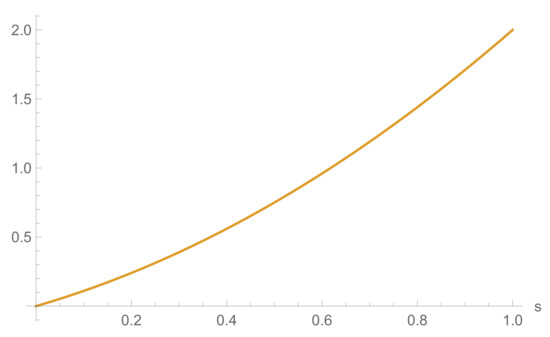
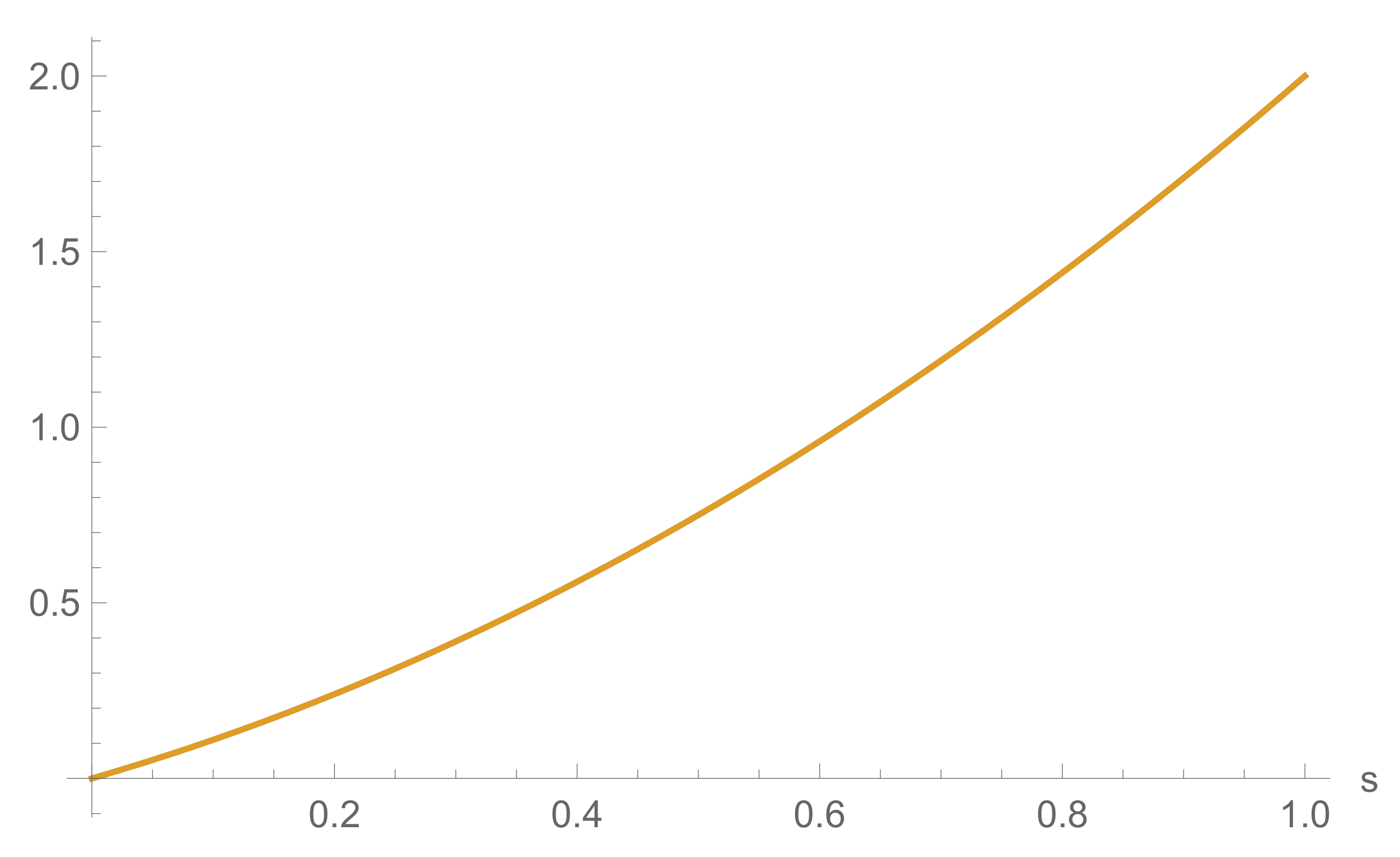
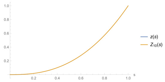
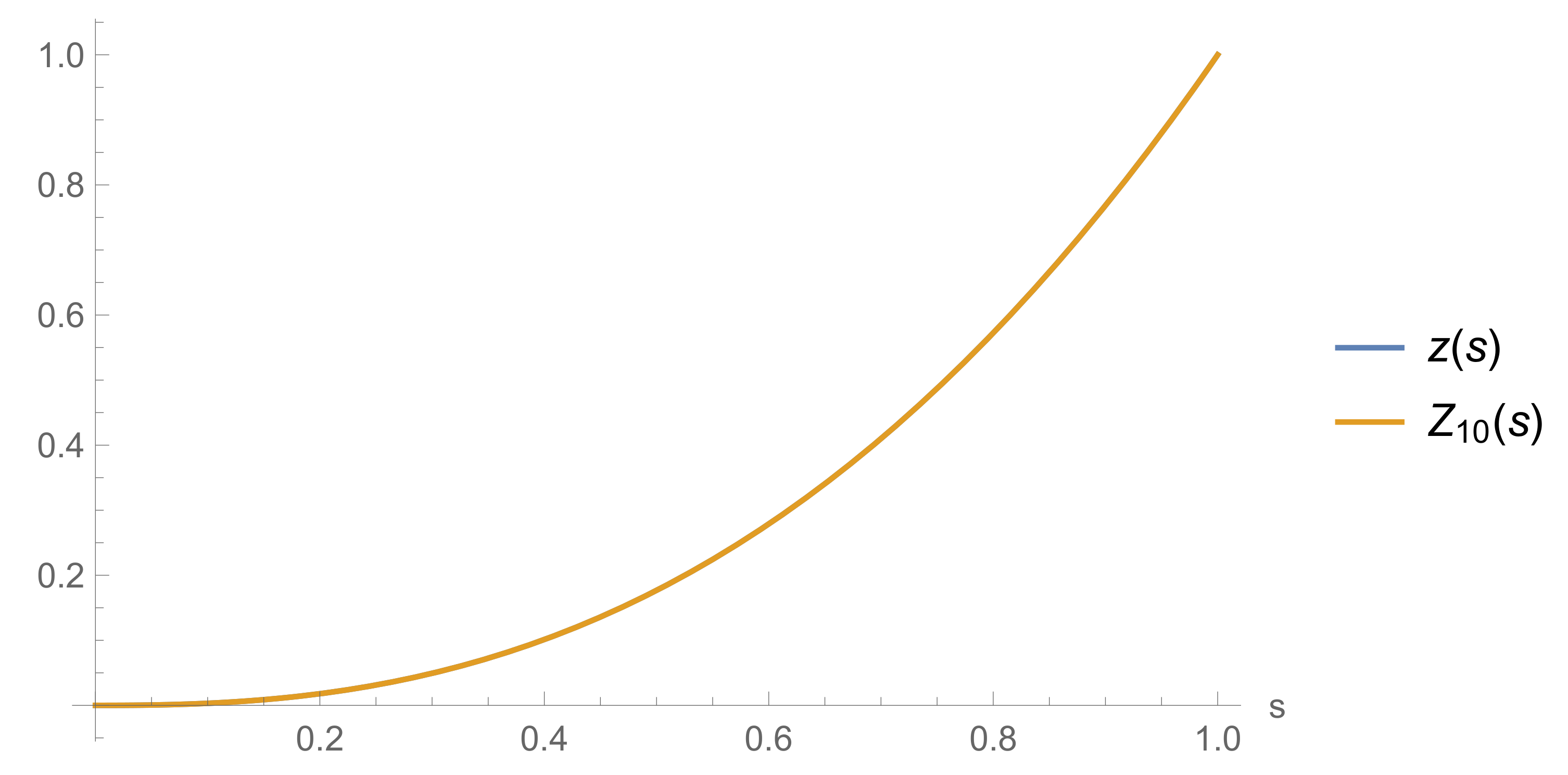
Figure 1. The graphs of $z\left(s\right)$ and $Z_5\left(s\right)$ for Example 1.

Example 2. 

Consider the delay fractional problem

$$\begin{array}{ccc}\hfill D^{2}z\left(s\right)& =& D^{\frac{s}{4}}z\left(s\right)+(sins)z\left(\frac{s}{3}\right)+r\left(s\right),0<s<1\hfill \end{array}$$

(63)

$$\begin{array}{c}z\left(0\right)=-2,z^{\prime }\left(0\right)=1,\hspace{1em}\hspace{1em}\hspace{1em}\hspace{1em}\hspace{1em}\hspace{1em}\hspace{1em}\hspace{1em}\hspace{1em}\hfill \end{array}$$

(64)

where

$$r\left(s\right)=2-\frac{2}{\mathrm{\Gamma }(3-\frac{s}{4})}{s}^{2-\frac{s}{4}}-\frac{1}{\mathrm{\Gamma }(2-\frac{s}{4})}{s}^{1-\frac{s}{4}}-(sins)\left(\frac{s^2}{9}+\frac{s}{3}-2\right).$$

(65)

The exact solution was given by

$$z\left(s\right)=s^2+s-2.$$

(66)

Let the approximate solution be given by

$$Z_5\left(s\right)=\sum _{k=0}^5{\nu }_{k}S{T}_k\left(s\right).$$

(67)

Then, using the proposed method, we obtained

$${\nu }_0=-1.1875000001, {\nu }_1=0.5, {\nu }_2=0.0625, {\nu }_3={\nu }_4={\nu }_5=0.$$

(68)

Thus,

$$Z_5\left(s\right)=-1.1875000001S{T}_0\left(s\right)+0.5S{T}_1\left(s\right)+0.0625S{T}_2\left(s\right)=-2.0000000001+s+s^2.$$

(69)

Let

$${ϵ}_5=max\left\{\right|z\left(0\right)-Z_5\left(0\right)|,|z\left(s_1\right)-Z_5\left(s_1\right)|,\dots ,|z\left(s_4\right)-Z_5\left(s_4\right)|,|z\left(1\right)-Z_5\left(1\right)\left|\right\}.$$

(70)

Then,${ϵ}_5={10}^{-10}$. The absolute error is reported in Table 2. The graphs of$z\left(s\right)$and$Z_5\left(s\right)$are presented in Figure 2.

Table 2. Absolute error for Example 2.

s	$|\mathit{z}\left(\mathit{s}\right)-{\mathit{Z}}_5\left(\mathit{s}\right)|$
0	${10}^{-10}$
0.1	${10}^{-10}$
0.2	${10}^{-10}$
0.3	${10}^{-10}$
0.4	${10}^{-10}$
0.5	${10}^{-10}$
0.6	${10}^{-10}$
0.7	${10}^{-10}$
0.8	${10}^{-10}$
0.9	${10}^{-10}$
1.0	${10}^{-10}$

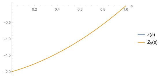
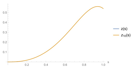
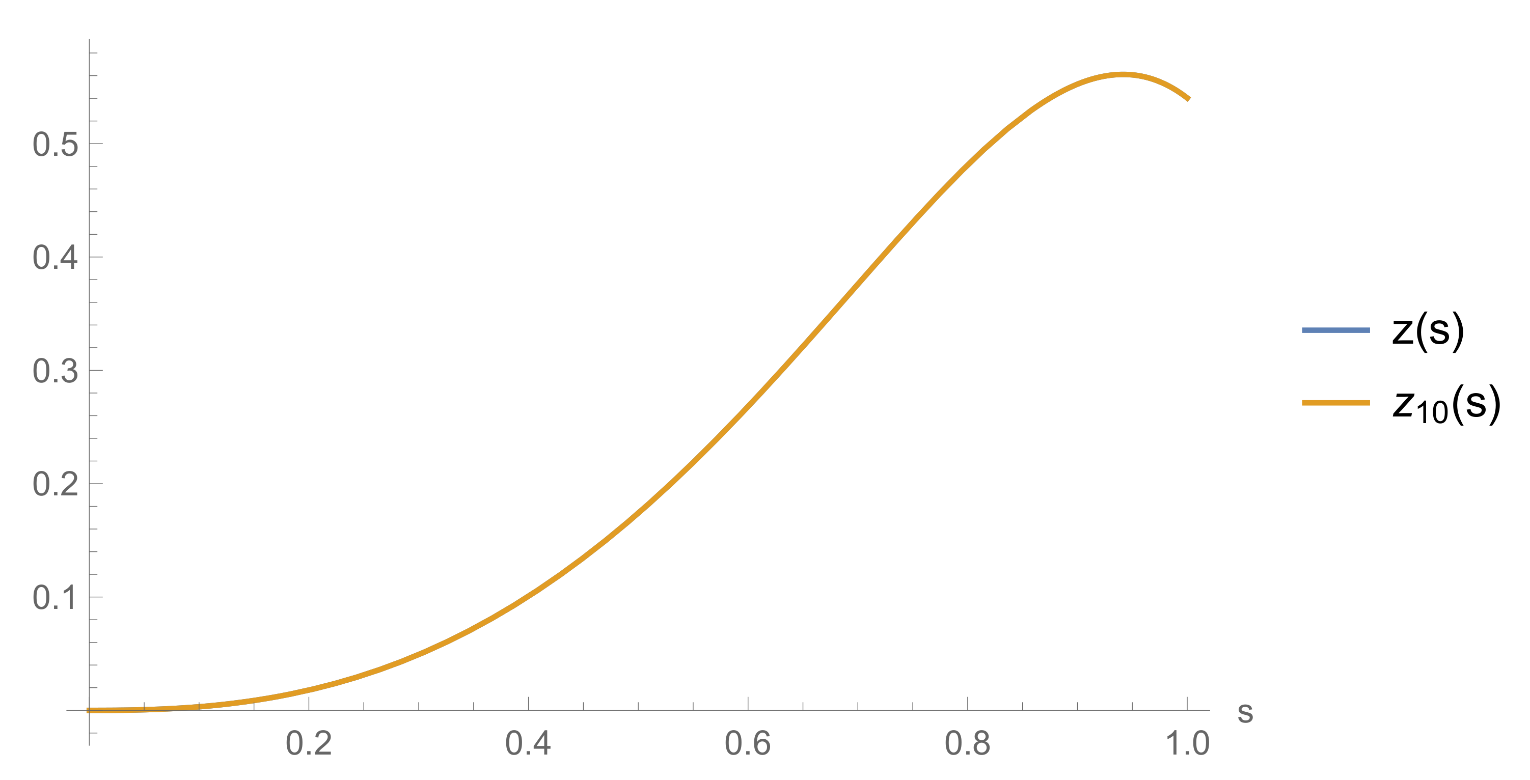
Figure 2. The graphs $z\left(s\right)$ and $Z_5\left(s\right)$ for Example 2.

Example 3. 

Consider the delay fractional problem

$$\begin{array}{ccc}\hfill D^{2}z\left(s\right)& =& D^{s}z\left(s\right)+z\left(\frac{s}{4}\right)+r\left(s\right),0<s<1\hfill \end{array}$$

(71)

$$\begin{array}{c}z\left(0\right)=0,z^{\prime }\left(0\right)=0,\hspace{1em}\hspace{1em}\hspace{1em}\hspace{1em}\hspace{1em}\hspace{1em}\hspace{1em}\hspace{1em}\hspace{1em}\hfill \end{array}$$

(72)

where

$$r\left(s\right)=\frac{15}{4}\sqrt{s}-\frac{15\sqrt{\pi }}{8\mathrm{\Gamma }\left(\frac{7}{2}-s\right)}{s}^{\frac{5-2s}{2}}-\frac{1}{32}{s}^{\frac{s}{2}}.$$

(73)

The exact solution was given by

$$z\left(s\right)=s^{\frac{5}{2}}.$$

(74)

Let the approximate solution be given by

$$Z_{10}\left(s\right)=\sum _{k=0}^{10}{\nu }_{k}S{T}_k\left(s\right).$$

(75)

Using the proposed method, we had

$$\begin{array}{c}{\nu }_0=\frac{256}{315\pi },{\nu }_1=\frac{512}{693\pi },{\nu }_2=\frac{256}{1001\pi },{\nu }_3=\frac{1024}{45045\pi },\hspace{1em}\hspace{1em}\hspace{1em}\hspace{1em}\hspace{1em}\hfill \end{array}$$

(76)

$$\begin{array}{c}{\nu }_4=\frac{-256}{153153\pi },{\nu }_5=\frac{512}{1616615\pi },{\nu }_6=\frac{-256}{2909907\pi },{\nu }_7=\frac{2048}{66927861\pi },\hfill \end{array}$$

(77)

$$\begin{array}{c}{\nu }_8=\frac{-2304}{185810725\pi },{\nu }_9=\frac{512}{91265265\pi },{\nu }_{10}=\frac{-2816}{1017958725\pi }.\hspace{1em}\hspace{1em}\hspace{1em}\hfill \end{array}$$

(78)

Let

$$ϵ\left(s\right)=|z\left(s\right)-Z_{10}\left(s\right)|.$$

(79)

The absolute error is reported in Table 3. The graphs of$z\left(s\right)$and$Z_{10}\left(s\right)$are presented in Figure 3.

Table 3. Absolute error for Example 3.

s	$|\mathit{z}\left(\mathit{s}\right)-{\mathit{Z}}_{10}\left(\mathit{s}\right)|$
0	$\hspace{1em}\hspace{1em}\hspace{1em}{10}^{-7}$
0.1	$1.0\times {10}^{-7}$
0.2	$1.0\times {10}^{-7}$
0.3	$5.3\times {10}^{-7}$
0.4	$5.0\times {10}^{-7}$
0.5	$4.3\times {10}^{-7}$
0.6	$1.9\times {10}^{-7}$
0.7	$1.0\times {10}^{-7}$
0.8	$3.1\times {10}^{-7}$
0.9	$4.1\times {10}^{-7}$
1.0	$4.9\times {10}^{-7}$

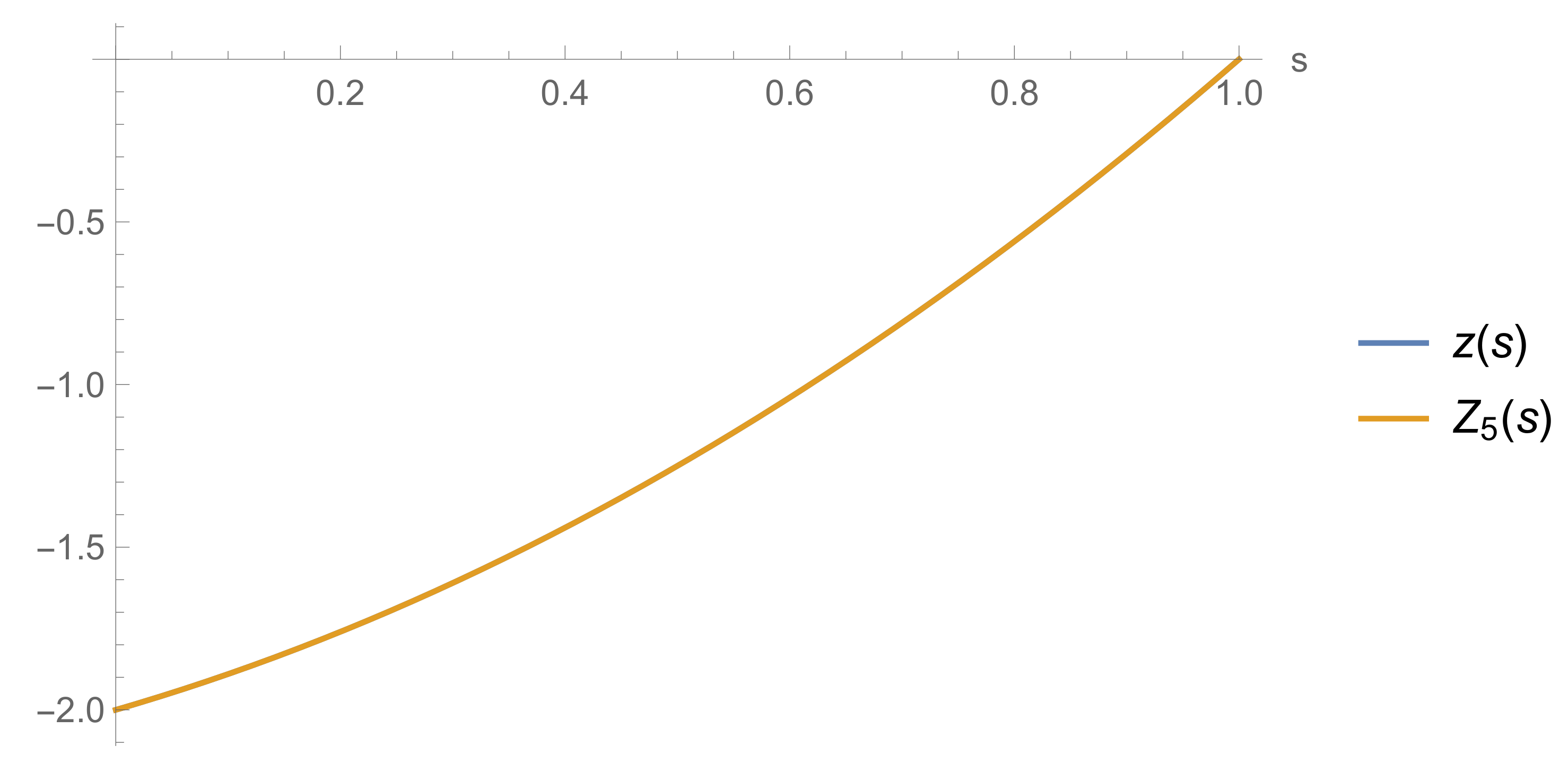
Figure 3. The graphs of $z\left(s\right)$ and $Z_{10}\left(s\right)$ for Example 3.

Example 4. 

Consider the delay fractional problem

$$\begin{array}{ccc}\hfill D^{2}z\left(s\right)& =& D^{s}z\left(s\right)+z\left(\frac{s}{3}\right)+r\left(s\right),0<s<1\hfill \end{array}$$

(80)

$$\begin{array}{c}z\left(0\right)=0,z^{\prime }\left(0\right)=0,\hspace{1em}\hspace{1em}\hspace{1em}\hspace{1em}\hspace{1em}\hspace{1em}\hspace{1em}\hspace{1em}\hfill \end{array}$$

(81)

where$r\left(s\right)$was chosen so that the exact solution was given by

$$z\left(s\right)=s^{\frac{5}{2}}cos\left(s^{\frac{5}{2}}\right).$$

(82)

Let the approximate solution be given by

$$Z_{10}\left(s\right)=\sum _{k=0}^{10}{\nu }_{k}S{T}_k\left(s\right).$$

(83)

Using the proposed method, we had

$$\begin{array}{c}{\nu }_0=0.220256,{\nu }_1=0.18058,{\nu }_2=0.035659,{\nu }_3=-0.0189969,\hspace{1em}\hspace{1em}\hspace{1em}\hspace{1em}\hspace{1em}\hfill \end{array}$$

(84)

$$\begin{array}{c}{\nu }_4=-0.0109545,{\nu }_5=-0.00258346,{\nu }_6=-0.000356888,{\nu }_7=0.0000498019,\hfill \end{array}$$

(85)

$$\begin{array}{c}{\nu }_8=0.0000219865,{\nu }_9=7.20851\times {10}^{-6},{\nu }_{10}=-2.72747\times {10}^{-7}.\hspace{1em}\hspace{1em}\hspace{1em}\hspace{1em}\hfill \end{array}$$

(86)

Let

$$ϵ\left(s\right)=|z\left(s\right)-Z_{10}\left(s\right)|.$$

(87)

The absolute error is reported in Table 4. The graphs of$z\left(s\right)$and$Z_{10}\left(s\right)$are presented in Figure 4.

Table 4. Absolute error for Example 4.

s	$|\mathit{z}\left(\mathit{s}\right)-{\mathit{Z}}_{10}\left(\mathit{s}\right)|$
0	$\hspace{1em}\hspace{1em}\hspace{1em}{10}^{-6}$
0.1	$1.6\times {10}^{-6}$
0.2	$1.5\times {10}^{-6}$
0.3	$7.2\times {10}^{-7}$
0.4	$6.7\times {10}^{-7}$
0.5	$5.8\times {10}^{-7}$
0.6	$5.1\times {10}^{-7}$
0.7	$4.9\times {10}^{-7}$
0.8	$4.5\times {10}^{-7}$
0.9	$4.1\times {10}^{-7}$
1.0	$4.0\times {10}^{-7}$

Figure 4. The graphs of $z\left(s\right)$ and $Z_{10}\left(s\right)$ for Example 4.

6. Conclusions

We presented an algorithm to solve a class of delay fractional initial value problems with the variable Caputo fractional derivative. We expanded the approximate solution using extended types of Chebyshev polynomials and then determined the coefficients using the operational matrix approach. We proved that the approximate solutions converged uniformly to the exact ones. We illustrated the efficiency of the presented approach through four examples. It was noticed that the computed errors were small, even if we considered a number of terms in the expansion. We chose examples where their exact solutions were available, so it was possible to compute the exact errors. The approximate solutions were very close to the exact ones, which indicated the efficiency of the presented approach in dealing with these types of problems, and, therefore, it is recommended to extend its use to other types of problems.

References

- Alshomrani, A.; Ullah, M.; Baleanu, D. Caputo SIR model for COVID-19 under optimized fractional order. Adv. Differ. Equ. 2021, 2021, 185. [Google Scholar] [CrossRef] [Scilit] [PubMed]
- Ahmad, S.; Ullah, R.; Baleanu, D. Mathematical analysis of tuberculosis control model using nonsingular kernel type Caputo derivative. Adv. Differ. Equ. 2021, 2021, 26. [Google Scholar] [CrossRef] [Scilit]
- Omay, T.; Baleanu, D. Fractional unit-root tests allowing for a fractional frequency flexible Fourier form trend: Predictability of COVID-19. Adv. Differ. Equ. 2021, 2021, 167. [Google Scholar] [CrossRef] [Scilit] [PubMed]
- Alomari, A.K.; Syam, M.; Anakira, N.R.; Jameel, A.F. Homotopy Sumudu transform method for solving applications in physics. Results Phys. 2020, 18, 103265. [Google Scholar] [CrossRef] [Scilit]
- Chen, Y.; Moore, K.L. Analytical stability bound for a class of delayed fractional-order dynamic systems. Nonlinear Dyn. 2002, 29, 191–200. [Google Scholar] [CrossRef] [Scilit]
- Caglar, H.; Caglar, N.; Ozer, M. B-spline solution of non-linear singular boundary value problems arising in physiology. Chaos Solitons Fractals 2009, 39, 1232–1237. [Google Scholar] [CrossRef] [Scilit]
- Shahmorad, S.; Ostadzad, M.H.; Baleanu, D. A Tau-like numerical method for solving fractional delay integro-differential equations. Appl. Numer. Math. 2020, 151, 322–336. [Google Scholar] [CrossRef] [Scilit]
- Syam, M.; Al-Refai, M. First order delay equations Implicit hybrid method. Alex. Eng. J. 2020, 59, 2677–2681. [Google Scholar] [CrossRef] [Scilit]
- Tassaddiq, A.; Yaseen, M.; Yousaf, A.; Srivastava, R. A cubic B-spline collocation method with new approximation for the numerical treatment of the heat equation with classical and non-classical boundary conditions. Phys. Scr. 2021, 96, 045212. [Google Scholar] [CrossRef] [Scilit]
- Zheng, W.; Huang, R.; Luo, Y.; Chen, Y.; Wang, X.; Chen, Y. A Look-up table based fractional order composite controller synthesis method for the PMSM speed servo system. Fractal Fract. 2022, 6, 47. [Google Scholar] [CrossRef] [Scilit]
- Agarwal, R.P.; Al-Hutami, H.; Ahmad, B. A Langevin-type q-variant system of nonlinear fractional integro-difference equations with nonlocal boundary conditions. Fractal Fract. 2022, 6, 45. [Google Scholar] [CrossRef] [Scilit]
- Reyaz, R.; Mohamad, A.; Lim, Y.; Saqib, M.; Shafie, S. Analytical solution for impact of Caputo-Fabrizio fractional derivative on MHD casson fluid with thermal radiation and chemical reaction effects. Fractal Fract. 2022, 6, 38. [Google Scholar] [CrossRef] [Scilit]
- Sene, N. Analytical solutions of a class of fluids models with the Caputo fractional derivative. Fractal Fract. 2022, 6, 35. [Google Scholar] [CrossRef] [Scilit]
- Zhu, C.G.; Kang, W.S. Numerical solution of Burgers-Fisher equation by cubic B-spline quasi-interpolation. Appl. Math. Comp. 2010, 216, 2679–2686. [Google Scholar] [CrossRef] [Scilit]
- Kashkari, B.; Syam, M. A numerical approach for investigating a special class of fractional Riccati equation. Results Phys. 2000, 17, 103080. [Google Scholar] [CrossRef] [Scilit]
- Abdelhakem, M.; Mahmoud, D.; Baleanu, D.; El-kady, M. Shifted ultraspherical pseudo-Galerkin method for approximating the solutions of some types of ordinary fractional problem. Adv. Differ. Equ. 2021, 2021, 110. [Google Scholar] [CrossRef] [Scilit]
- Coronel-Escamilla, A.; Gómez-Aguilar, J. A novel predictor–corrector scheme for solving variable-order fractional delay differential equations involving operators with Mittag–Leffler kernel. Discret. Contin. Dyn. Syst. Ser. 2020, 13, 561–574. [Google Scholar] [CrossRef] [Scilit]
- Daftardar-Gejji, V.; Sukale, Y.; Bhalekar, S. A new predictor-corrector method for fractional differential equations. Appl. Math. Comput. 2014, 244, 158–182. [Google Scholar] [CrossRef] [Scilit]
- Daftardar-Gejji, V.; Jafari, H. An iterative method for solving non linear functional equations. J. Math. Anal. Appl. 2006, 316, 753–763. [Google Scholar] [CrossRef] [Scilit]
- Gülsu, M.; Gürbüz, B.; Öztürk, Y.; Sezer, M. Laguerre polynomial approach for solving linear delay difference equations. Appl. Math. Comput. 2011, 217, 6765–6776. [Google Scholar] [CrossRef] [Scilit]
- Gürbüz, B.; Sezer, M. Laguerre polynomial solutions of a class of initial and boundary value problems arising in science and engineering fields. Acta Phys. Pol. 2000, 130, 194–197. [Google Scholar] [CrossRef] [Scilit]
- Gurbuz, B.; Sezerm, M. Laguerre polynomial approach for solving nonlinear Klein-Gordon equations. Malays. J. Math. Sci. 2017, 11, 191–203. [Google Scholar]
- Gurbuz, B.; Sezer, M. Modified operational matrix method for second-order nonlinear ordinary differential equations with quadratic and cubic terms. Int. J. Optim. Control Theor. Appl. 2020, 10, 218–225. [Google Scholar] [CrossRef] [Scilit]
- Kashkari, B.; Syam, M. Fractional-order Legendre operational matrix of fractional integration for solving the Riccati equation with fractional order. Appl. Math. Comput. 2016, 290, 281–291. [Google Scholar] [CrossRef] [Scilit]
- Gorenflo, R.; Luchko, Y. Operational method for solving generalized Abel integral equations of second kind. Integral Transform. Spec. Funct. 1997, 5, 47–58. [Google Scholar] [CrossRef] [Scilit]
- Hadid, S.B.; Luchko, Y.F. An operational method for solving fractional differential equations of an arbitrary real order. Panamer. Math. J. 1996, 6, 57–73. [Google Scholar]
- Lorenzo, C.F.; Hartley, T.T. Variable order and distributed order fractional operators. Nonlinear Dyn. 2002, 29, 57–98. [Google Scholar] [CrossRef] [Scilit]
- Samko, S.G.; Ross, B. Integration and differentiation to a variable fractional order. Integral Transform. Spec. Funct. 1993, 1, 277–300. [Google Scholar] [CrossRef] [Scilit]
- Samko, S. Fractional integration and differentiation of variable order: An overview. Nonlinear Dyn. 2013, 71, 653–662. [Google Scholar] [CrossRef] [Scilit]
- Naylor, A.W.; Sell, G.R. Linear Operator Theory in Engineering and Science, 2nd ed.; Applied Mathematical Sciences; Springer: New York, NY, USA; Berlin, Germany, 1982; Volume 40. [Google Scholar]
Publisher’s Note: MDPI stays neutral with regard to jurisdictional claims in published maps and institutional affiliations. |
© 2022 by the authors. Licensee MDPI, Basel, Switzerland. This article is an open access article distributed under the terms and conditions of the Creative Commons Attribution (CC BY) license (https://creativecommons.org/licenses/by/4.0/).