The Dynamical Analysis of a Biparametric Family of Six-Order Ostrowski-Type Method under the Möbius Conjugacy Map

Abstract

In this paper, a family of Ostrowski-type iterative schemes with a biparameter was analyzed. We present the dynamic view of the proposed method and study various conjugation properties. The stability of the strange fixed points for special parameter values is studied. The parameter spaces related to the critical points and dynamic planes are used to visualize their dynamic properties. Eventually, we find the most stable member of the biparametric family of six-order Ostrowski-type methods. Some test equations are examined for supporting the theoretical results.

1. Introduction

In many fields including mathematics, physics and engineering, the problem of solving nonlinear equations $f\left(x\right)=0$ is involved where $f:D\subseteq \mathrm{R}\to \mathrm{R}$ is a differentiable function defined in an open interval D. It is almost impossible to find the exact solutions of nonlinear equations, so an iterative method is used to obtain the as accurate as possible approximate solutions. The most classic iterative scheme is Newton’s iterative method [1]. In recent years, many researchers have devoted themselves to designing a class of high-order iterative methods to solve nonlinear equations by using different techniques to improve Newton’s scheme. Rational linear function method [2], combination method [3] and weight-function method [4] are often used to generate new iterative methods or to improve the convergence order of known methods.

Ostrowski’s method [5] is the optimal fourth-order method under the Kung–Traub’s conjecture [6]. A variant of Ostrowski-type methods using the weight-function procedure is proposed by Chun [7], which is given by

$$\left\{\begin{array}{c}{y}_n=x_n-\frac{f\left(x_n\right)}{f^{\prime }\left(x_n\right)},\hfill \\ w_n=y_n-\frac{f\left(x_n\right)}{f\left(x_n\right)-2f\left(y_n\right)}\frac{f\left(y_n\right)}{f^{\prime }\left(x_n\right)},\hfill \\ x_{n+1}=w_n-H\left(u_n\right)\frac{f\left(w_n\right)}{f^{\prime }\left(x_n\right)},\hfill \end{array}\right.$$

(1)

where $u_n=\frac{f\left(y_n\right)}{f\left(x_n\right)}$ and $H\left(u_n\right)$ represents a weight function. In view of Theorem 1 of Reference [6], if function $H\left(u_n\right)$ satisfies the conditions $H\left(0\right)=1$, $H^{\prime }\left(0\right)=2$, and $|H^{″}\left(0\right)|<\infty$, then the above iteration scheme is sixth-order. In the current study, we will select the concrete form of $H\left(u_n\right)$ with two-parameter t, $k\in C$: $H\left(u_n\right)=\frac{t+(2t+k)u_n}{t+k{u}_n}.$

Hence, we obtain the following biparametric family of sixth-order method (OM):

$$\left\{\begin{array}{c}{y}_n=x_n-\frac{f\left(x_n\right)}{f^{\prime }\left(x_n\right)},\hfill \\ w_n=y_n-\frac{f\left(x_n\right)}{f\left(x_n\right)-2f\left(y_n\right)}\frac{f\left(y_n\right)}{f^{\prime }\left(x_n\right)},\hfill \\ x_{n+1}=w_n-\frac{tf\left(x_n\right)+(2t+k)f\left(y_n\right)}{tf\left(x_n\right)+kf\left(y_n\right)}\frac{f\left(w_n\right)}{f^{\prime }\left(x_n\right)}.\hfill \end{array}\right.$$

(2)

The fixed point operator of (2) or iteration function is:

$$R_f\left(z\right)=z-\frac{f\left(z\right)}{f^{\prime }\left(z\right)}-\frac{f\left(z\right)}{f\left(z\right)-2f\left(y\right)}\frac{f\left(y\right)}{f^{\prime }\left(z\right)}-\frac{tf\left(z\right)+(2t+k)f\left(y\right)}{tf\left(z\right)+kf\left(y\right)}\frac{f\left(w\right)}{f^{\prime }\left(z\right)},$$

(3)

where:

$$y=z-\frac{f\left(z\right)}{f^{\prime }\left(z\right)},w=y-\frac{f\left(z\right)}{f\left(z\right)-2f\left(y\right)}\frac{f\left(y\right)}{f^{\prime }\left(z\right)}.$$

(4)

For simplicity, we mark w as $w\left(z\right)$.

For arbitrary members (except for $t=0$ and $k=0$) of the OM family (2), the speed of convergence is similar. Our main interest is the stability of the OM family in this paper. Since the dynamic properties of the iterative method provide us with important information about the stability and reliability of members. In these respects, several scholars described the dynamical behavior of different iterative families (see [4,6,8,9,10,11]). For example, Maroju et al. [11] analyzed the dynamical behavior of Chebyshev–Halley family. Magreñán [12] studied some anomalies in the fourth-order Jarrat family. These iterative methods are all one-parameter iterative schemes. We will investigate the dynamic properties of rational functions $R_f\left(z\right)$ on low-degree polynomials associated with the biparametric family (2) with the help of complex dynamics tools [13]. This analysis allows us to reject poorly behaved members and select the most stable ones.

Now, we review some basic dynamical concepts (see [8,9,14]) which will be used in paper. Given a rational function $R:\overline{C}\to \overline{C}$, where $\overline{C}$ is the Riemann sphere, the orbit of a point $z_0\in \overline{C}$ is defined as

$$\left\{z_0,R\left(z_0\right),R^2\left(z_0\right),\cdots ,R^n\left(z_0\right),\cdots \right\}.$$

Moreover, a fixed point $z_0$ can be divided into the following four types:

(a)

Attractor if $|R^{\prime }\left(z_0\right)|<1$.

(b)

Superattractor if $|R^{\prime }\left(z_0\right)|=0$.

(c)

Repulsor if $|R^{\prime }\left(z_0\right)|>1$.

(d)

Parabolic if $|R^{\prime }\left(z_0\right)|=1$.

The basin of attraction of an attractor $z^{*}$ is defined as

$$\mathcal{A}\left(z^{*}\right)=\left\{z_0\in \overline{C}:R^n\left(z_0\right)\to z^{*},n\to \infty \right\}.$$

This article is divided into seven sections. Section 2 briefly describes the preliminary results of the dynamics on $\overline{C}$. In Section 3, we obtain the strange fixed points of $R_f\left(z\right)$ and investigate its stability. In Section 4, the relevant properties of the free critical points are described. Section 5 presents the parameter space associated with free critical points and the dynamic plane of family (2) elements. In Section 6, we conduct numerical experiments on the proposed method and the existing methods. In Section 7, we make a short summary.

2. Preliminary Results

Theorem 1 (The Scaling Theorem).

Let $f\left(z\right)$ be an analytic function on the Riemann sphere, and let $\mathsf{\Gamma }\left(z\right)=az+b,a\ne 0$, be an affine map. If $h\left(z\right)=f\circ \mathsf{\Gamma }\left(z\right)$, then the fixed points operator (3) $R_f$ is analytically conjugated to $R_h$ by Γ, that is $\mathsf{\Gamma }\circ R_h\circ {\mathsf{\Gamma }}^{-1}\left(z\right)=R_f\left(z\right)$.

Proof. 

With the iteration function $R\left(z\right)$, we have:

$$\begin{array}{ccc}{R}_h\left({\mathsf{\Gamma }}^{-1}\left(z\right)\right)\hfill & =& {\mathsf{\Gamma }}^{-1}\left(z\right)-\frac{h\left({\mathsf{\Gamma }}^{-1}\left(z\right)\right)}{h^{\prime }\left({\mathsf{\Gamma }}^{-1}\left(z\right)\right)}-\frac{h\left({\mathsf{\Gamma }}^{-1}\left(z\right)\right)}{h\left({\mathsf{\Gamma }}^{-1}\left(z\right)\right)-2h({\mathsf{\Gamma }}^{-1}\left(z\right)-\frac{h\left({\mathsf{\Gamma }}^{-1}\left(z\right)\right)}{h^{\prime }\left({\mathsf{\Gamma }}^{-1}\left(z\right)\right)})}\frac{h({\mathsf{\Gamma }}^{-1}\left(z\right)-\frac{h\left({\mathsf{\Gamma }}^{-1}\left(z\right)\right)}{h^{\prime }\left({\mathsf{\Gamma }}^{-1}\left(z\right)\right)})}{h^{\prime }\left({\mathsf{\Gamma }}^{-1}\left(z\right)\right)}\\ \hfill & & -\frac{th\left({\mathsf{\Gamma }}^{-1}\left(z\right)\right)+(k+2t)h({\mathsf{\Gamma }}^{-1}\left(z\right)-\frac{h\left({\mathsf{\Gamma }}^{-1}\left(z\right)\right)}{h^{\prime }\left({\mathsf{\Gamma }}^{-1}\left(z\right)\right)})}{th\left({\mathsf{\Gamma }}^{-1}\left(z\right)\right)+kh({\mathsf{\Gamma }}^{-1}\left(z\right)-\frac{h{\mathsf{\Gamma }}^{-1}\left(z\right)}{h^{\prime }\left({\mathsf{\Gamma }}^{-1}\left(z\right)\right)})}\frac{h\left(w\left({\mathsf{\Gamma }}^{-1}\left(z\right)\right)\right)}{h^{\prime }\left({\mathsf{\Gamma }}^{-1}\left(z\right)\right)}.\end{array}$$

(5)

since:

$$h\circ {\mathsf{\Gamma }}^{-1}\left(z\right)=f\left(z\right),$$

(6)

$${(h\circ {\mathsf{\Gamma }}^{-1})}^{\prime }\left(z\right)=\frac{1}{a}{h}^{\prime }\left({\mathsf{\Gamma }}^{-1}\left(z\right)\right),$$

(7)

we obtain:

$$h^{\prime }\left({\mathsf{\Gamma }}^{-1}\left(z\right)\right)=a{(h\circ {\mathsf{\Gamma }}^{-1})}^{\prime }\left(z\right)=a{f}^{\prime }\left(z\right),$$

(8)

and

$$h^{″}\left({\mathsf{\Gamma }}^{-1}\left(z\right)\right)=a^2{f}^{″}\left(z\right).$$

(9)

Using (6) and (8), we obtain:

$$\begin{array}{ccc}{R}_h\left({\mathsf{\Gamma }}^{-1}\left(z\right)\right)\hfill & =& {\mathsf{\Gamma }}^{-1}\left(z\right)-\frac{f\left(z\right)}{a{f}^{\prime }\left(z\right)}-\frac{f\left(z\right)}{f\left(z\right)-2h({\mathsf{\Gamma }}^{-1}\left(z\right)-\frac{f\left(z\right)}{a{f}^{\prime }\left(z\right)})}\frac{h({\mathsf{\Gamma }}^{-1}\left(z\right)-\frac{f\left(z\right)}{a{f}^{\prime }\left(z\right)})}{a{f}^{\prime }\left(z\right)}\\ \hfill & & -\frac{tf\left(z\right)+(k+2t)h({\mathsf{\Gamma }}^{-1}\left(z\right)-\frac{f\left(z\right)}{a{f}^{\prime }\left(z\right)})}{tf\left(z\right)+kh({\mathsf{\Gamma }}^{-1}\left(z\right)-\frac{f\left(z\right)}{a{f}^{\prime }\left(z\right)})}\frac{h\left(w\left({\mathsf{\Gamma }}^{-1}\left(z\right)\right)\right)}{a{f}^{\prime }\left(z\right)}.\end{array}$$

(10)

Therefore:

$$\begin{array}{lll}{R}_f\left(z\right)& =& \mathsf{\Gamma }\circ R_h\circ {\mathsf{\Gamma }}^{-1}\left(z\right)=\mathsf{\Gamma }\left(R_h\left({\mathsf{\Gamma }}^{-1}\left(z\right)\right)\right)=a{R}_h\left({\mathsf{\Gamma }}^{-1}\left(z\right)\right)+b\\ \hfill & =& a{\mathsf{\Gamma }}^{-1}\left(z\right)-\frac{f\left(z\right)}{f^{\prime }\left(z\right)}-\frac{f\left(z\right)}{f\left(z\right)-2h({\mathsf{\Gamma }}^{-1}\left(z\right)-\frac{f\left(z\right)}{a{f}^{\prime }\left(z\right)})}\frac{h({\mathsf{\Gamma }}^{-1}\left(z\right)-\frac{f\left(z\right)}{a{f}^{\prime }\left(z\right)})}{f^{\prime }\left(z\right)}\\ \hfill & & -\frac{tf\left(z\right)+(k+2t)h({\mathsf{\Gamma }}^{-1}\left(z\right)-\frac{f\left(z\right)}{a{f}^{\prime }\left(z\right)})}{tf\left(z\right)+kh({\mathsf{\Gamma }}^{-1}\left(z\right)-\frac{f\left(z\right)}{a{f}^{\prime }\left(z\right)})}\frac{h\left(w\left({\mathsf{\Gamma }}^{-1}\left(z\right)\right)\right)}{f^{\prime }\left(z\right)}+b\\ \hfill & =& z-\frac{f\left(z\right)}{f^{\prime }\left(z\right)}-\frac{f\left(z\right)}{f\left(z\right)-2h({\mathsf{\Gamma }}^{-1}\left(z\right)-\frac{f\left(z\right)}{a{f}^{\prime }\left(z\right)})}\frac{h({\mathsf{\Gamma }}^{-1}\left(z\right)-\frac{f\left(z\right)}{a{f}^{\prime }\left(z\right)})}{f^{\prime }\left(z\right)}\\ \hfill & & -\frac{tf\left(z\right)+(k+2t)h({\mathsf{\Gamma }}^{-1}\left(z\right)-\frac{f\left(z\right)}{a{f}^{\prime }\left(z\right)})}{tf\left(z\right)+kh({\mathsf{\Gamma }}^{-1}\left(z\right)-\frac{f\left(z\right)}{a{f}^{\prime }\left(z\right)})}\frac{h\left(w\left({\mathsf{\Gamma }}^{-1}\left(z\right)\right)\right)}{f^{\prime }\left(z\right)}.\end{array}$$

(11)

We then just need to prove that $h({\mathsf{\Gamma }}^{-1}\left(z\right)-\frac{f\left(z\right)}{a{f}^{\prime }\left(z\right)})=f\left(y\right)$ and $h\left(w\left({\mathsf{\Gamma }}^{-1}\left(z\right)\right)\right)=f\left(w\left(z\right)\right)$. First prove that $h({\mathsf{\Gamma }}^{-1}\left(z\right)-\frac{f\left(z\right)}{a{f}^{\prime }\left(z\right)})=f\left(y\right)$. By using the Taylor expansion of $h({\mathsf{\Gamma }}^{-1}\left(z\right)-\frac{f\left(z\right)}{a{f}^{\prime }\left(z\right)})$ about ${\mathsf{\Gamma }}^{-1}\left(z\right)$ and (9), we have:

$$\begin{array}{lll}h({\mathsf{\Gamma }}^{-1}\left(z\right)-\frac{f\left(z\right)}{a{f}^{\prime }\left(z\right)})\hfill & =& h\left({\mathsf{\Gamma }}^{-1}\left(z\right)\right)-h^{\prime }\left({\mathsf{\Gamma }}^{-1}\left(z\right)\right)\frac{f\left(z\right)}{a{f}^{\prime }\left(z\right)}+h^{″}\left({\mathsf{\Gamma }}^{-1}\left(z\right)\right)\frac{f{\left(z\right)}^2}{2a^2{f}^{\prime }{\left(z\right)}^2}\\ \hfill & & -h^{‴}\left({\mathsf{\Gamma }}^{-1}\left(z\right)\right)\frac{f{\left(z\right)}^3}{6a^3{f}^{\prime }{\left(z\right)}^3}+\cdots \\ \hfill & =& f^{″}\left(z\right)\frac{f{\left(z\right)}^2}{2f^{\prime }{\left(z\right)}^2}-f^{″\prime }\left(z\right)\frac{f{\left(z\right)}^3}{6f^{\prime }{\left(z\right)}^3}+\cdots \\ \hfill & =& f(z-\frac{f\left(z\right)}{f^{\prime }\left(z\right)})\\ \hfill & =& f\left(y\right).\end{array}$$

(12)

The prove that $h\left(w\left({\mathsf{\Gamma }}^{-1}\left(z\right)\right)\right)=f\left(w\right)$. Because:

$$\begin{array}{c}h\left(w\right)=h(z-\frac{h\left(z\right)}{h^{\prime }\left(z\right)}-\frac{h\left(z\right)}{h\left(z\right)-2h(z-\frac{h\left(z\right)}{h^{\prime }\left(z\right)})}\frac{h(z-\frac{h\left(z\right)}{h^{\prime }\left(z\right)})}{h^{\prime }\left(z\right)}).\hfill \end{array}$$

(13)

Replacing z with ${\mathsf{\Gamma }}^{-1}\left(z\right)$ in (13), we obtain:

$$\begin{array}{lll}h\left(w\left({\mathsf{\Gamma }}^{-1}\left(z\right)\right)\right)\hfill & =& h({\mathsf{\Gamma }}^{-1}\left(z\right)-\frac{h\left({\mathsf{\Gamma }}^{-1}\left(z\right)\right)}{h^{\prime }\left({\mathsf{\Gamma }}^{-1}\left(z\right)\right)}-\frac{h\left({\mathsf{\Gamma }}^{-1}\left(z\right)\right)}{h\left({\mathsf{\Gamma }}^{-1}\left(z\right)\right)-2h({\mathsf{\Gamma }}^{-1}\left(z\right)-\frac{h\left({\mathsf{\Gamma }}^{-1}\left(z\right)\right)}{h^{\prime }\left({\mathsf{\Gamma }}^{-1}\left(z\right)\right)})}\frac{h({\mathsf{\Gamma }}^{-1}\left(z\right)-\frac{h\left({\mathsf{\Gamma }}^{-1}\left(z\right)\right)}{h^{\prime }\left({\mathsf{\Gamma }}^{-1}\left(z\right)\right)})}{h^{\prime }\left({\mathsf{\Gamma }}^{-1}\left(z\right)\right)})\\ \hfill & =& h({\mathsf{\Gamma }}^{-1}\left(z\right)-\frac{f\left(z\right)}{a{f}^{\prime }\left(z\right)}-\frac{f\left(z\right)}{f(z-2h({\mathsf{\Gamma }}^{-1}\left(z\right)-\frac{f\left(z\right)}{a{f}^{\prime }\left(z\right)}))}\frac{h({\mathsf{\Gamma }}^{-1}\left(z\right)-\frac{f\left(z\right)}{a{f}^{\prime }\left(z\right)})}{a{f}^{\prime }\left(z\right)})\\ \hfill & =& h(\frac{z-b}{a}-\frac{f\left(z\right)}{a{f}^{\prime }\left(z\right)}-\frac{f\left(z\right)}{f\left(z\right)-2f\left(y\right)}\frac{f\left(y\right)}{a{f}^{\prime }\left(y\right)})\\ \hfill & =& h\left(\frac{1}{a}(y-\frac{f\left(z\right)}{f\left(z\right)-2f\left(y\right)}\frac{f\left(y\right)}{a{f}^{\prime }\left(z\right)}-b)\right)\\ \hfill & =& f\circ \mathsf{\Gamma }\left(\frac{1}{a}(y-\frac{f\left(z\right)}{f\left(z\right)-2f\left(y\right)}\frac{f\left(y\right)}{a{f}^{\prime }\left(z\right)}-b)\right)\\ \hfill & =& f(y-\frac{f\left(z\right)}{f\left(z\right)-2f\left(y\right)}\frac{f\left(y\right)}{a{f}^{\prime }\left(z\right)})\\ \hfill & =& f\left(w\right).\end{array}$$

(14)

From (14), we obtain $\mathsf{\Gamma }\circ R_h\circ {\mathsf{\Gamma }}^{-1}\left(z\right)=R_f\left(z\right)$; then this proof is completed. □

The above theorem shows that it allows us to conjugate the dynamical behavior of one operator with the behavior related to another, conjugated by an affine application.

Definition 1.

Let $\mathcal{F}:\mathrm{X}\subset \overline{\mathcal{C}}\to \mathrm{X}$ and $\mathcal{O}:\mathrm{Y}\subset \overline{\mathcal{C}}\to \mathrm{Y}$ be two functions (representing two dynamical systems). We say that $\mathcal{F}$ is conjugate to $\mathcal{O}$ via Γ if there exists an isomorphism $\mathsf{\Gamma }:\mathrm{Y}\to \mathrm{X}$ such that $\mathcal{F}\circ \mathsf{\Gamma }=\mathsf{\Gamma }\circ \mathcal{O}$. Such a map Γ is called a conjugacy [15].

According to Theorem 1 which was proven in [4], we find:

Theorem 2.

Let $\mathcal{F}$ and $\mathcal{O}$ be defined by Definition 1 be of class $C^1$ and are conjugate to each other via the diffeomorphic conjugacy Γ. Moreover, let ξ be a fixed point of $\mathcal{O}$. Then, the following hold:

(a) 

The fixed points property remains invariant under a topological conjugacy Γ, that is:

$$\xi =\mathcal{O}\left(\xi \right)\begin{array}{cccc}if& and& only& if\end{array}\mathsf{\Gamma }\left(\xi \right)=\mathcal{F}\left(\mathsf{\Gamma }\left(\xi \right)\right).$$

(b) 

The Poincar$\acute{e}$ characteristic multiplier [10] of ξ by $\mathcal{O}$, denoted by $m(\mathcal{O},\xi )$, is invariant under a diffeomorphic conjugacy Γ, that is:

$$m(\mathsf{\Gamma }\circ \mathcal{O}\circ {\mathsf{\Gamma }}^{-1},\mathsf{\Gamma }\left(\xi \right))={\mathcal{F}}^{\prime }\left(\mathsf{\Gamma }\left(\xi \right)\right)={\mathcal{O}}^{\prime }\left(\xi \right)=m(\mathcal{O},\xi ).$$

Remark 1.

Results of Theorem 2 state that a conjugacy Γ indeed preserves the dynamical behavior between the two dynamical systems; for example, if $\mathcal{F}$ and $\mathcal{O}$ are conjugate to each other via Γ, and ξ is a fixed point of $\mathcal{O}$, then $\mathsf{\Gamma }\left(\xi \right)$ is a fixed point of $\mathcal{F}$. The converse is also true, that is, let ξ be a fixed point of $\mathcal{F}$, then ${\mathsf{\Gamma }}^{-1}\left(\xi \right)$ is a fixed point of $\mathcal{O}$; Furthermore, ξ is a critical point or free critical point of $\mathcal{O}$, then $\mathsf{\Gamma }\left(\xi \right)$ is a critical point or free critical point of $\mathcal{F}$. The converse is also true. The above is based on the invariance properties of the fixed point and its multiplier under the conjugacy.

Furthermore, we discover $\mathcal{F}=\mathsf{\Gamma }\circ \mathcal{O}\circ {\mathsf{\Gamma }}^{-1}$ and ${\mathcal{F}}^n=(\mathsf{\Gamma }\circ \mathcal{O}\circ {\mathsf{\Gamma }}^{-1})\circ (\mathsf{\Gamma }\circ \mathcal{O}\circ {\mathsf{\Gamma }}^{-1})\cdots \circ (\mathsf{\Gamma }\circ \mathcal{O}\circ {\mathsf{\Gamma }}^{-1})=\mathsf{\Gamma }\circ {\mathcal{O}}^n\circ {\mathsf{\Gamma }}^{-1}$. If $\mathcal{F}$ and $\mathcal{O}$ are extra invertible, we can also find ${\mathcal{F}}^{-1}=\mathsf{\Gamma }\circ {\mathcal{O}}^{-1}\circ {\mathsf{\Gamma }}^{-1}$ and ${\mathcal{F}}^{-n}=\mathsf{\Gamma }\circ {\mathcal{O}}^{-n}\circ {\mathsf{\Gamma }}^{-1}$, besides the topological conjugacy, $\mathsf{\Gamma }$ maps an orbit:

$$\cdots ,{\mathcal{O}}^{-2}\left(y\right),{\mathcal{O}}^{-1}\left(y\right),y,\mathcal{O}\left(y\right),{\mathcal{O}}^2\left(y\right),\cdots$$

of $\mathcal{O}$ onto an orbit:

$$\cdots ,{\mathcal{F}}^{-2}\left(x\right),{\mathcal{F}}^{-1}\left(x\right),x,\mathcal{F}\left(x\right),{\mathcal{F}}^2\left(x\right),\cdots$$

of $\mathcal{F}$, where $x=\mathsf{\Gamma }\left(y\right)$. From this, we find that the order of points is preserved. Thus, the orbits of the two maps behave similarly under homeomorphism $\mathsf{\Gamma }$. According to the invariant properties of the fixed point, the multiplier as well as the scaling theorem, it is assuredly of value to study the dynamics of a conjugated map if simplified through conjugacy $\mathsf{\Gamma }$.

3. Fixed Points and Stability

Due to topological invariance, we transform $R_f$ in (3) into $\Omega$ by a linear fractional M$\ddot{\mathrm{o}}$bius conjugacy map $M\left(z\right)=\frac{z-a}{z-b},(a\ne b)$ fulfilling:

$$\Omega (z;a,b,t,k)=\frac{I(z;a,b,t,k)}{\Theta (z;a,b,t,k)},$$

(15)

when applied to an arbitrary prototype quadratic polynomial $f\left(z\right)=(z-a)(z-b)$, where I and $\Theta$ are rational polynomials whose coefficients are dependent upon parameters $a,b,t,k$. One of our aims is to make coefficients of both I and $\Theta$ be minimally dependent on parameters. According to the previously mentioned conjugate, we find that all the coefficients of both I and $\Theta$ are only dependent upon t and k, and independent of a and b. Consequently, with the aid of the symbolic operation capability of Mathematica [16], (15) can be written as

$$\Omega (z;t,k)=-z^4\frac{\sigma (z;t,k)}{\mu (z;t,k)},$$

(16)

where:

$$\sigma (z;t,k)=-k-2t+(k+2t)z+2t{z}^2+(k+2t)z^3+t{z}^4,$$

(17)

$$\mu (z;t,k)=-t-(k+2t)z-2t{z}^2-(k+2t)z^3+(k+2t)z^4,$$

(18)

We then apply a special treatment to t, the cases for values $t\in \left\{\frac{1}{2},-\frac{1}{2},1,-1\right\}$. The aim is to simplify the rational function also to reduce the dependence on the parameters even further. In this study, the more interesting one is $t=1$, which corresponds to the fixed point operator of the following form:

$$\Omega (z;k)=\Omega (z;1,k)=\frac{z^4\left[-2-k+(2+k)z+2z^2+(2+k)z^3+z^4\right]}{1+(2+k)z+2z^2+(2+k)z^3-(2+k)z^4}.$$

(19)

We will investigate the fixed points of $\Omega$ and their stability. The fixed points of $\Omega (z;k)$ are given by the roots of:

$$\Omega (z;k)-z=\frac{z(z-1)\left[1+(3+k)z+(5+k)z^2+3(3+k)z^3+(5+k)z^4(3+k)z^5+z^6\right]}{1+(2+k)z+2z^2+(2+k)z^3-(2+k)z^4}=\frac{z(z-1)\rho \left(z\right)}{\zeta \left(z\right)},$$

(20)

where we handily denote:

$$\rho \left(z\right)=1+(3+k)z+(5+k)z^2+3(3+k)z^3+(5+k)z^4(3+k)z^5+z^6,$$

(21)

$$\zeta \left(z\right)=1+(2+k)z+2z^2+(2+k)z^3-(2+k)z^4.$$

(22)

The conjugacy map we consider is a M$\ddot{\mathrm{o}}$bius transformation $\mathsf{\Gamma }\left(z\right)=M\left(z\right)=\frac{z-a}{z-b}$, with the following properties:

$$\left(i\right)\mathsf{\Gamma }\left(a\right)=0,\left(ii\right)\mathsf{\Gamma }\left(b\right)=\infty ,\left(iii\right)\mathsf{\Gamma }(\infty )=1.$$

This enable us to discover that $z=0$ and $z=\infty$ are clearly two fixed points of $\Omega =\mathsf{\Gamma }\circ R_f\circ {\mathsf{\Gamma }}^{-1}$, with $\mathsf{\Gamma }\left(z\right)=\frac{z-a}{z-b}$, respectively, corresponding to fixed points a and b of $R_f$ or the roots a and b of polynomial $f\left(z\right)=(z-a)(z-b)$. Furthermore, $0,\infty$ are free of the parameter k. In addition, they are super-attractive points and suggest the critical points of $\Omega (z;k)$.

Nonetheless, because $\Omega \left(0\right)=0$, $\Omega (\infty )=\infty$, that is, their orbits draw near themselves, such fixed points would show a tiny impact on the dynamics. Fixed points not excluding $\left\{0,\infty \right\}$ are termed as strange fixed points which are different from the roots of $f\left(z\right)$. In order to find further strange fixed points, we need to solve the equations $\Omega (z;k)-z=0$ in (20) for z with given values of k.

3.1. Strange Fixed Points

We first check the existence of k-values for common factors (divisors) of $\rho \left(z\right)$ and $\zeta \left(z\right)$. Additionally, both $\rho \left(z\right)$ and $\zeta \left(z\right)$ will be checked if they have a factor $(z-1)$. The following theorem best describes the relevant properties of such existence as well as explicit strange fixed points.

Theorem 3.

(a) 

If $k=-1$, then $\rho \left(z\right)$ and $\zeta \left(z\right)$ have a common factor $(z+1)$, the operator Ω has the strange fixed points $z=1,z=-1,z=-i\sqrt{\frac{1}{2}}(3\pm \sqrt{5}),i\sqrt{\frac{1}{2}(3\pm \sqrt{5})}$;

(b) 

If $k=-3$, then $\rho \left(z\right)$ and $\zeta \left(z\right)$ have two common factors $1+z^2$ and $1-z+z^2$, the operator Ω has the strange fixed points $z=1,z=-0.5\pm 0.866025i$;

(c) 

If $=-\frac{27}{7}$, then $\rho \left(z\right)$ has a factor $(z-1)$, the operator Ω has the strange fixed points $z=1\left(triple\right),z=-0.332631\pm 1.13238i,z=-0.238798\pm 0.812947i$;

(d) 

If $k=-5$, then $\zeta \left(z\right)$ has a factor $(z-1)$, the operator Ω has the strange fixed points $z=0.357785,z=2.79497,z=-0.367445\pm 1.27423i,z=-0.208934\pm 0.724541i$;

(e) 

For k satisfying $(k+1)(k+3)(k+\frac{27}{7})(k+5)\ne 0$, the strange fixed points are given by $z=1$ and the six roots of $\rho \left(z\right)=0$ in terms of parameter k.

Proof. 

(a), (b) Suppose that $\rho \left(z\right)=0$ and $\zeta \left(z\right)=0$ for some values of $z\in \overline{C}$. Observe that parameter k exists in a linear way in all coefficients of both polynomials. By eliminating k from the two polynomials, we obtain the relation: ${(1+z^2)}^2(1+z)(1-z+z^2)=0$. Hence, $(1+z)$, $1+z^2,{(1+z^2)}^2,(1-z+z^2)=0$ are candidates for common divisors of $\rho \left(z\right)$ and $\zeta \left(z\right)$. First, substituting $z=-1$, we find $\rho (-1)=6-3(3+k)=0$, $\zeta (-1)=-3-3k=0$, from which $k=-1$ is obtained. Indeed, $\rho \left(z\right)$ and $\zeta \left(z\right)$ reduce to, respectively, ${(1+z)}^2$$(1+3z^2+z^4)$ and $(1+z)(1+2z^2-z^3)$, as desired. Second, dividing both $\rho \left(z\right)$ and $\zeta \left(z\right)$ by $1+z^2$ yields the identical remainder as $-k-3$, from which the remainder becomes zero for $k=-3$. Indeed, $\rho \left(z\right)$ and $\zeta \left(z\right)$ reduce to, respectively, $(1+z^2)(1-z+z^2)(1+z+z^2)$ and $(1+z^2)(1-z+z^2)$. Accordingly, we find that $(1-z+z^2)$ is indeed a common factor of $\rho \left(z\right)$ and $\zeta \left(z\right)$. Thus, dividing both $\rho \left(z\right)$ and $\zeta \left(z\right)$ by $1-z+z^2$ yields the remainder, respectively, as $-3k-9$,$(2k+6)-(k+3)$ and the remainder becomes zero for $k=-3$. After that, it is the same as the previous common factor $(1+z^2)$. Third, the direct division of $\rho \left(z\right)$ by ${(1+z^2)}^2$ is performed, then its remainder as $(k+3)z^3-(k+2)z^{2-k-2}$, which cannot be zero for any k-values. The rest of the proof only needs to substitute the corresponding $\rho \left(z\right)$ and $\zeta \left(z\right)$ into (20) and solve its roots to be the strange fixed points.

(c)

We find that $\rho \left(z\right)$ has a factor for $k=-\frac{27}{7}$ via solving $\rho \left(1\right)=27+7k=0$. In fact, for $k=-\frac{27}{7}$, we also obtain ${\rho }^{\prime }\left(1\right)=0$. Hence, $\rho \left(z\right)$ has a factor ${(z-1)}^2$ for $k=-\frac{27}{7}$. Then, $\rho \left(z\right)=\frac{1}{7}{(z-1)}^2(7+8z+17z^2+8z^3+7z^4)$, $\zeta \left(z\right)=\frac{1}{7}(7-13z+14z^2-13z^3+13z^4)$. The rest of its proof is trivial.

(d)

If $(z-1)$ is a divisor of $\zeta \left(z\right)$, then $\zeta \left(1\right)=5+k=0$. For a value of $k=-5$, we discover $\zeta \left(z\right)=(z-1)(-1-2z+3z^3)$. As a result, we obtain the strange fixed points z satisfying $\rho \left(z\right)=1-2z-6z^3-2z^5+z^6=0$. The rest of the proof is similar to (a).

(e)

It is straightforward for us to claim the results. We numerically obtain the strange fixed points z satisfying $\rho \left(z\right)=0$ for given values of $k\notin \left\{-1,-3,-\frac{27}{7},-5\right\}$; detailed analysis will be shown later.

□

3.2. Stability of the Strange Fixed Points

To study the stability of fixed points, we need to compute the first derivative of $\Omega$ from (19):

$${\Omega }^{\prime }(z;k)=-\frac{z^3(1+z^2)\chi \left(z\right)}{\zeta {\left(z\right)}^2}.$$

(23)

where:

$$\begin{array}{ccc}\chi \left(z\right)\hfill & =& 8+4k+(2+7k+3k^2)z-4(7+4k+k^2)z^2-2(22+13k+k^2)z^3\\ \hfill & & -4(7+4k+k^2)z^4(2+7k+3k^2)z^5+(8+4k)z^6.\end{array}$$

(24)

$$\begin{array}{ccc}\zeta \left(z\right)\hfill & =& 1+(2+k)z+2z^2+(2+k)z^3-(2+k)z^4.\end{array}$$

(25)

We first check the existence of k-values for common factors (divisors) of $\chi \left(z\right)$ and $\zeta \left(z\right)$. Additionally, $\chi \left(z\right)$ and $\zeta \left(z\right)$ will be checked for whether they have divisors $z^3$, $1+z^2$. The following theorem best describes the relevant properties of such existence as well as explicit strange fixed points.

Theorem 4.

(a) 

If $k=-5$, then ${\Omega }^{\prime }(z;k)=\frac{6z^3(1+z^2)(2-3z-3z^3+2z^4)}{{(-1-2z+3z^3)}^2}$;

(b) 

If $k=-1$, then ${\Omega }^{\prime }(z;k)=-\frac{2z^3(1+z^2)(2-5z-5z^3+2z^4)}{{(-1-2z+3z^3)}^2}$;

(c) 

If $k=-3$, then ${\Omega }^{\prime }(z;k)=4z^3$;

(d) 

If $k=-2$, then ${\Omega }^{\prime }(z;k)=-\frac{12z^5{(1+z^2)}^2}{{(1+2z^2)}^2}$;

(e)

If $(k+5)(k+1)(k+3)(k+2)\ne 0$, then we can demonstrate the desired stability of z by varying parameter k with the aid of Theorem 6.

Proof. 

(a), (b), (c) Suppose that $\chi \left(z\right)=0$ and $\zeta \left(z\right)=0$ for some values of z. By eliminating k from the two polynomials, we obtain the relation: $(z-1)(z+1)(1+z^2)(1-z+z^2)(1+z^2-4z^3+2z^4-4z^5)=0$. Hence, $(z-1)$,$(z+1)$,$(1+z^2)$,$(1-z+z^2)$ are candidates for common divisors of $\chi \left(z\right)$ and $\zeta \left(z\right)$. After checking constraints $\chi \left(1\right)=\zeta \left(1\right)=0$,$\chi (-1)=\zeta (-1)=0$, we find that $k=-5,-1$ yielding common divisors. By checking zero remainders when dividing both $\chi \left(z\right)$ and $\zeta \left(z\right)$ by $(1+z^2)$ and $(1-z+z^2)$, respectively, we find $k=-3$ yielding common divisors.

(d)

For $\chi \left(z\right)$ to have a factor z, we require $k=-2$ by solving $\chi \left(0\right)=8+4k=0$ for k. For $\chi \left(z\right)$ to have a factor $(1+z^2)$, we require its remainder $(8k^2+40k+48)z=0$, from which $k=-3,-2$.

(c)

If $\zeta \left(z\right)$ has a factor $(1+z^2)$, then its remainder is $-k-3$, from which the remainder becomes zero for $k=-3$.

The rest of the above proof only needs to substitute the corresponding $\chi \left(z\right)$ and $\zeta \left(z\right)$ into (23).

(e)

If k satisfies $(k+5)(k+1)(k+3)(k+2)\ne 0$, then the graphical stability of z yields the desired results.

□

Regarding the stability of the strange fixed points, we conduct research in two cases. The first is the stability of the strange fixed points for special k-values; the second is the stability of the other strange fixed points corresponding to the root of $\rho \left(z\right)$ and $z=1$.

Using the results of Theorem 4 to describe the stability of the fixed points in Theorem 3 in terms of parameter k. Table 1 presents the stability results of the first case.

Table 1. Stability of strange fixed points $\xi$ for special k-values.

k	$\mathit{\xi }$				No. of $\mathit{\xi }$
	$|{\Omega }^{\prime }(\mathit{\xi };\mathit{k})|$: ${\mathit{m}}^{\mathit{w}}$
−1	1	−1	$-i\sqrt{\frac{1}{2}(3\pm \sqrt{5})}$	$i\sqrt{\frac{1}{2}(3\pm \sqrt{5})}$	6
	6:g	3.5:g	7.81025:g	7.81025:g
−5	0.357785	2.79497	−0.367445 ± 1.27423i	−0.208934 ± 0.724541i	6
	11.787:g	11.7871:g	5.73:g	5.72996:g
−27/7	1((triple)	−0.332631 ± 1.13238i	−0.238798 ± 0.812947i		7
	1:f	4.91055:g	4.91066:g
−3	1	−0.5 ± 0.866025i			3
	4:g	4:g
−2	−0.732786 ± 0.68046i	0.0732949 ± 0.673932i	0.159491 ± 1.46648i		6
	4.86704:g	10.8788:g	10.8786:g

^ω|Ω^′(ξ;k)|: m denotes that ξ is attractive, parabolic and repulsive, if m = e(|Ω^′| < 1), m = f(|Ω^′| = 1), m = g(|Ω^′| > 1), respectively.

Theorem 5.

Let $k\notin \left\{-5,-1,-3,-2,-\frac{27}{7}\right\}$, then the relevant properties of the strange fixed point $z=1$ are as follows:

(a) 

If $k=-4$, then $z=1$ is a superattracting point;

(b) 

If $|k+\frac{251}{63}|<\frac{8}{63}$, then $z=1$ is an attractive point;

(c) 

If $|k+\frac{251}{63}|=\frac{8}{63}$, then $z=1$ is a parabolic fixed point;

(d) 

At last, if $|k+\frac{251}{63}|>\frac{8}{63}$, then $z=1$ is a repulsive point.

Proof. 

Substituting $z=1$ into Equation (23), we obtain:

$$|{\Omega }^{\prime }(1;k)|=8\left|\frac{4+k}{5+k}\right|.$$

It is easy to confirm that $|{\Omega }^{\prime }(1;-4)|=0$. Again, $8|\frac{4+k}{5+k}|\le 1$ is equivalent to $8|4+k|\le |5+k|$. Let $k=x+iy$ be an arbitrary complex number. Then:

$${|4+k|}^2={(4+x)}^2+y^{2}and{|5+k|}^2={(5+x)}^2+y^2.$$

So:

$$64\left[{(4+x)}^2+y^2\right]\le {(5+x)}^2+y^2.$$

By simplifying:

$$63x^2+63y^2+502x+999\le 0.$$

That is:

$${\left(x+\frac{251}{63}\right)}^2+y^2=\left(\frac{8}{63}\right).$$

Therefore:

$$\begin{array}{cccccc}|{\Omega }^{\prime }(1;k)|\le 1\hfill & if& and& only& if& |k+\frac{251}{63}|\le \frac{8}{63}.\end{array}$$

□

Remark 2.

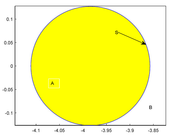
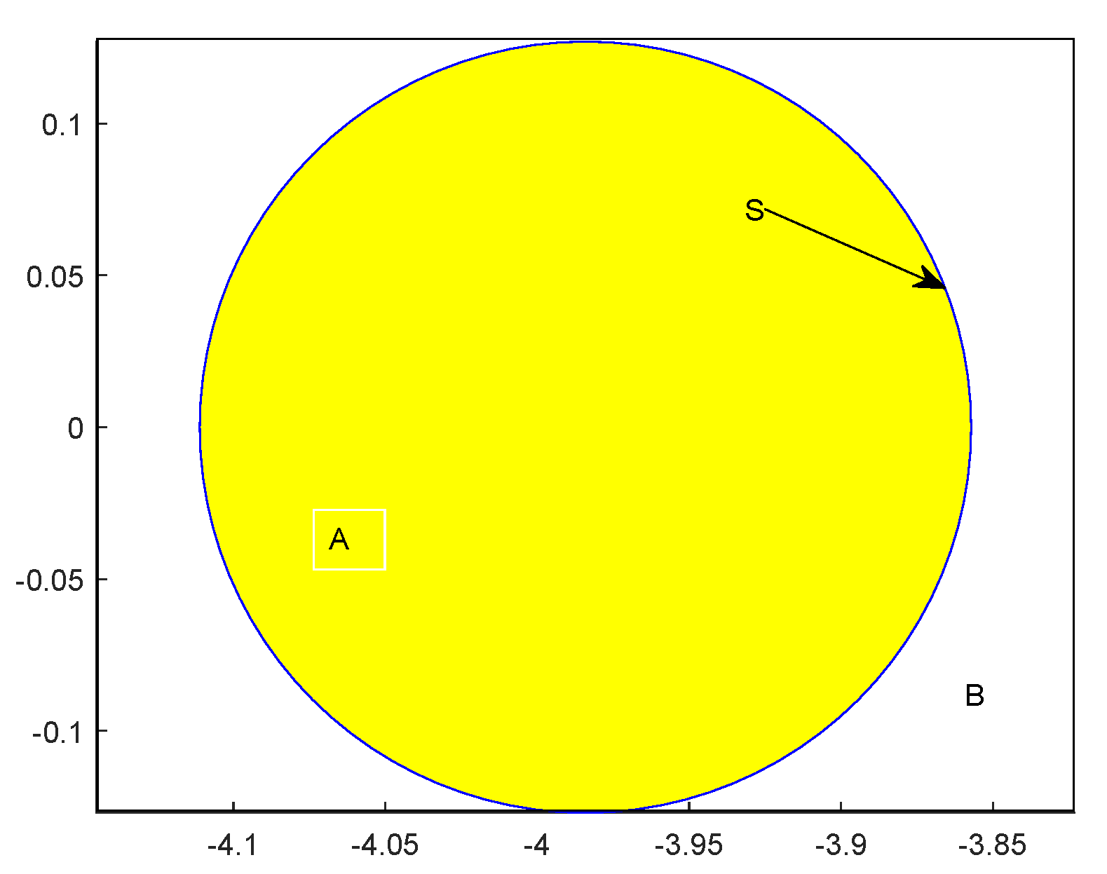
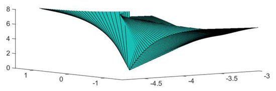
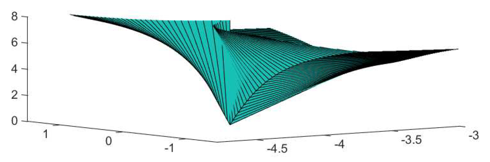
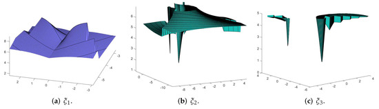
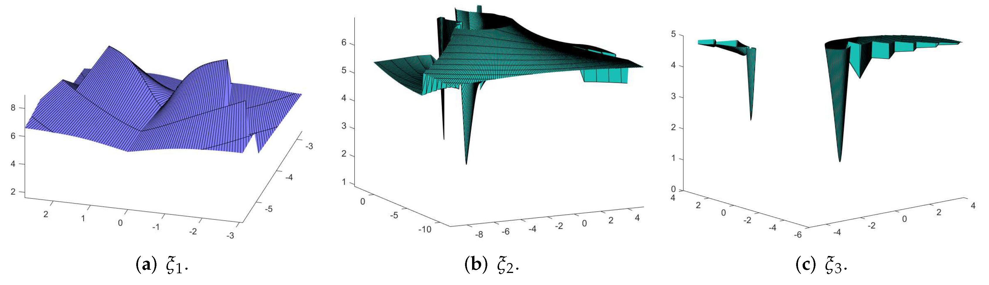
For later use, we conveniently let $A=\left\{k\in C:|{\Omega }^{\prime }(1;k)|<1\right\}$, $S=\{k\in C:|{\Omega }^{\prime }(1;k)|$$=1\}$ and $S=\left\{k\in C:|{\Omega }^{\prime }(1;k)|>1\right\}$. Then, $A,S,B$ indicate the sets where the strange fixed point $z=1$ becomes attractive, repulsive, and indifferent, respectively. As seen in Figure 1, S is the boundary between A as a circle of radius $\frac{8}{63}$ centered at $\left(-\frac{251}{63},0\right)$. Furthermore, Figure 2 shows a stability surface with $z=1$ (independent of parameter k).

Figure 1. Stability circle S for the strange fixed point $z=1$.

Figure 2. Stability surfaces of strange fixed point $z=1$.

Lemma 1.

If $\xi \in \overline{C}$ is the root of $\rho \left(z\right)$ defined in (21), then $\frac{1}{\xi }$ is also a root of $\rho \left(z\right)$ for any $k\in C$ and any $z\in \overline{C}$.

Proof. 

Let $\rho \left(z\right)=0$. Substituting $\frac{1}{\xi }$ into $\rho \left(z\right)$ for z, we obtain:

$$\begin{array}{lll}\rho \left(\frac{1}{\xi }\right)\hfill & =& 1+(3+k)\frac{1}{\xi }+(5+k)\frac{1}{{\xi }^2}+3(3+k)\frac{1}{{\xi }^3}+(5+k)\frac{1}{{\xi }^4}+(3+k)\frac{1}{{\xi }^5}+\frac{1}{{\xi }^6}\\ \hfill & =& \frac{{\xi }^6+(3+k){\xi }^5+(5+k){\xi }^4+3(3+k){\xi }^3+(5+k){\xi }^2+(3+k)\xi +1}{{\xi }^6}\\ \hfill & =& \frac{\rho \left(\xi \right)}{{\xi }^6}\\ \hfill & =& 0.\end{array}$$

(26)

This completes the proof. □

Corollary 1.

If $\xi \in \overline{C}$ is a fixed point of Ω defined in (19), then $\frac{1}{\xi }$ is also a fixed point of Ω.

Proof. 

Based on the fact that $\Omega$ is conjugate to $\Omega$ via conjugacy $\mathsf{\Gamma }\left(z\right)=\frac{1}{z}$. yThus, let $\mathrm{X}=\mathrm{Y}=\overline{C}$, $\mathcal{O}=\mathcal{F}=\Omega$ in Theorem 2, then Theorem 2 (b) completes this proof. □

Lemma 2.

Let $(k+5)(k+1)(k+3)(k+2)(k+\frac{27}{7})\ne 0$ and ${\xi }_1,{\xi }_2,{\xi }_3\in C\backslash \left\{0\right\}$ be three roots of $\rho \left(z\right)$. Then, $\rho \left(z\right)$ can be expressed as the product of three second-degree polynomials as follows:

$$\rho \left(z\right)=\prod _{i=1}^3(1+d_{i}z+z^2)=\prod _{i=1}^3(z-{\xi }_i)\left(z-\frac{1}{{\xi }_i}\right),$$

where $d_i=-\left({\xi }_i+\frac{1}{{\xi }_i}\right)$ or ${\xi }_i=\frac{-d_i-\sqrt{{d_i}^2-4}}{2}$ for $1\le i\le 3$ in terms of k.

Proof. 

In view of Lemma 1 and Corollary 1, we find that if $\xi \ne 0$ is a strange fixed point of $\Omega (z;k)$ found from the roots of $\rho \left(z\right)=0$ for $k\notin \left\{-5,-1,-3,-2,-\frac{27}{7}\right\}$, then so is $\frac{1}{\xi }$.

Hence, the above factorization is valid. Then $\prod _{i=1}^3(z-{\xi }_i)\left(z-\frac{1}{{\xi }_i}\right)$ is easily acquired under the six-degree polynomials $\rho \left(z\right)$. $(1+d_i\left(z\right)+z^2)$ can be obtained by expanding $\left(z-\frac{1}{{\xi }_i}\right)$, it is clear that $d_i=-\left({\xi }_i+\frac{1}{{\xi }_i}\right)$ holds.

In order to continue to analyze the stability of the other fixed points from the root of $\rho \left(z\right)$, we need to find the root of $\rho \left(z\right)$ first by solving $\rho \left(z\right)=1+(3+k)z+(5+k)z^2+3(3+k)z^3+(5+k)z^4+(3+k)z^5+z^6=0$. By comparing the expansion of ${\prod }_{i=1}^3(1+d_{i}z+z^2)$ with the coefficients of the same order term of $\rho \left(z\right)$, we find that the following three equations are related to $d_1,d_2,d_3$:

$$\left\{\begin{array}{c}{d}_1+d_2+d_3=3+k,\hfill \\ 3+d_1{d}_2+d_1{d}_3+d_2{d}_3=5+k,\hfill \\ 2d_1+2d_2+2d_3+d_1{d}_2{d}_3=3(3+k).\hfill \end{array}\right.$$

(27)

We eliminate variables $d_2,d_3$ in (27) using the strong symbolic operation ability of Mathematica to ultimately access a decic equation in $d_1$ beneath:

$${d_1}^3-(3+k){d_1}^2+(2+k)d_1-(3+k)=0.$$

For convenience, we let $\Phi (d_1;k)$ denote ${d_1}^3-(3+k){d_1}^2+(2+k)d_1-(3+k)$. Eliminating $d_1,d_3$ and $d_1,d_2$, respectively, we then obtain a unique decic equation in $c\in \left\{d_1,d_2,d_3\right\}$ as follows:

$$\Phi (c;k)=0.$$

Now, we calculate the roots of $\Phi (c;k)$ and attain:

$$\begin{array}{c}{d}_1\left(k\right)=\frac{3+k}{3}-\frac{\sqrt[3]{2}(-3-3k-k^2)}{3·n\left(k\right)}+\frac{n\left(k\right)}{3·\sqrt[3]{2}},\hfill \\ d_2\left(k\right)=\frac{3+k}{3}-\frac{(1+i\sqrt{3})(-3-3k-k^2)}{3·\sqrt[3]{4}·n\left(k\right)}-\frac{(1-i\sqrt{3}·n\left(k\right))}{6·\sqrt[3]{2}},\hfill \\ d_3\left(k\right)=\frac{3+k}{3}-\frac{(1-i\sqrt{3})(-3-3k-k^2)}{3·\sqrt[3]{4}·n\left(k\right)}-\frac{(1+i\sqrt{3}·n\left(k\right))}{6·\sqrt[3]{2}}.\hfill \end{array}$$

where:

$$n\left(k\right)=\sqrt[3]{81+36k+9k^2+2k^3+3\sqrt{3}·\sqrt{239+204k+86k^2+24k^3+3k^4}}.$$

Then, substituting $d_i\left(k\right)$ for ${\xi }_i=\frac{-d_i-\sqrt{{d_i}^2-4}}{2},i=1,2,3$. The result is a k-dependent strange fixed point of $\Omega$. □

The stability surfaces of the strange fixed points dependent on parameter k are illustrated in Figure 3.

Figure 3. Stability surfaces of the strange fixed points ${\xi }_i,i=1,2,3$.

Lemma 3.

If $\xi \in \overline{C}$ is the root of $\chi \left(z\right)$ defined in (24), then $\frac{1}{\xi }$ is also a root of $\chi \left(z\right)$ for any $k\in C$ and any $z\in \overline{C}$.

Proof. 

As in the proof of Lemma 1, we obtain by direct calculation that $\chi \left(\frac{1}{\xi }\right)=\frac{\chi \left(\xi \right)}{{\xi }^6}$, because $\chi \left(\xi \right)=0$, proof completed. □

Theorem 6.

Let z be a strange fixed point of $\Omega (z;k)$ satisfying $\rho \left(z\right)=0$. Then, the following holds:

$${\Omega }^{\prime }(z;k)={\Omega }^{\prime }\left(\frac{1}{z};k\right).$$

(28)

Proof. 

The derivative of $\Omega$ is ${\Omega }^{\prime }(z;k)=-\frac{z^3(1+z^2)\chi \left(z\right)}{{\zeta \left(z\right)}^2}$. Substituting $\frac{1}{z}$ into ${\Omega }^{\prime }(z;k)$ for z and knowing from the proof of Lemma 3 that $\chi \left(\frac{1}{z}\right)=\frac{\chi \left(z\right)}{z^6}$, eventually, we obtain ${\Omega }^{\prime }\left(\frac{1}{z};k\right)=-\frac{(1+z^2)\chi \left(z\right)}{z^{11}{\zeta \left(\frac{1}{z}\right)}^2}$. As a result, it continues to check the relation:

$$\frac{z^3}{{\zeta \left(z\right)}^2}=\frac{1}{z^{11}{\zeta \left(\frac{1}{z}\right)}^2}.$$

By direct computation:

$$\begin{array}{c}\frac{z^3}{{\zeta \left(z\right)}^2}-\frac{1}{z^{11}{\zeta \left(\frac{1}{z}\right)}^2}=\frac{z^{14}{\zeta \left(\frac{1}{z}\right)}^2-{\zeta \left(z\right)}^2}{z^{11}{\zeta \left(z\right)}^2{\zeta \left(\frac{1}{z}\right)}^2}=\frac{-1-(k+1)z+k{z}^2+2z^3-2z^5-k{z}^6+(1+k)z^7+z^8}{z^{11}{\zeta \left(z\right)}^2{\zeta \left(\frac{1}{z}\right)}^2}·\rho \left(z\right)=0.\hfill \end{array}$$

is found. This completes the proof. □

The following lemma depicts how to find the super-attraction point under the strange fixed point of conjugated maps $\Omega (z;k)$ for some values of k. We need to concurrently solve $\rho \left(z\right)=\chi \left(z\right)=0$ for some values of k; in this way, the super-attractors of $\Omega (z;k)$ can be found. We first eliminate the parameter k from $\rho \left(z\right)=\chi \left(z\right)=0$, resulting in a polynomial over z with degree 16:

$${(1+z)}^2(1+z^2)(1-z+z^2)(1+6z^2-9z^3+12z^4-16z^5+12z^6-9z^7+6z^8+z^{10})=0.$$

In view of Theorem 6, there are only eight pairs super-attractors denoted by $\left(z_i,\frac{1}{z_i}\right)$ for $1\le i\le 8$, the stability of $z_i$ and $\frac{1}{z_i}$ are the same. Then, after solving ${\Omega }^{\prime }(z;k)=0$ for k numerically, we achieve the following Lemma deeming the needed super-attractors:

Lemma 4.

Let $z_1=-1,z_2=i,z_3=0.5+0.866025i,z_4=-0.791164+2.35788i,z_5=-0.255105-0.966913i,z_6=-0.127905+0.381192i,z_7=0.215007+0.976613i,z_8=0.959167$$+0.282841i$. Then $\left(z_i,\frac{1}{z_i}\right),(i=1,2,\cdots ,8)$ are super-attractors of $\Omega (z;k)$, respectively, for eight values of $k\in \{0,-3,-3.33333+9.87028\times {10}^{-7}i,-0.870604-2.7565i,-1.2134-1.08719\times {10}^{-6}i,$$-0.87065+2.7565\left.i,-2.78296+2.96051\times {10}^{-6}i,-3.77916-2.48912\times {10}^{-7}i\right\}$ or $\{-1,$$-2,-3+5.64784\times {10}^{-13}i,-2.23529+0.297382i,-3.50312+1.25267\times {10}^{-6}i,-2.23529-0.297381i,-2.71908-4.18506\times {10}^{-6}i,-4.79253\left.-2.27167\times {10}^{-7}i\right\}$.

4. Critical Points and Free Critical Points

The critical points of map $\Omega (z;k)$ are defined as the roots of ${\Omega }^{\prime }(z;k)=0$. From this known fact, each basin of attraction contains at least one free critical point. Operator $R_f\left(z\right)$ has as critical point 0, ∞ along with the roots of this sixth degree polynomial $\chi \left(z\right)$ where 0 and ∞ are related to a and b. Critical points that are different from 0 and ∞ are defined as free critical points. We are interested due to the orbital behavior of the free critical points, and we will deal with the free critical points which depend on parameter k.

Regarding the free critical points, we also divide the study into two parts such as the fixed points. One is to find the corresponding critical points for some special parameter valve k; the other is to find the critical points corresponding to the root of $\chi \left(z\right)$.

In view of Theorem 4, the free critical points for special k-values can easily be found and shown in Table 2.

Table 2. Free critical points $\xi$ for special k-values.

k	$\mathit{\eta }$	No. of $\mathit{\eta }$
−5	±i, 0.557699, 1.79308, −0.425391 ± 0.90501i	6
−1	±i, 0.360048, 2.77741, −0.318729 ± 0.947846i	6
−3		0
−2	i (double), −i (double)	4
−27/7	±i, 0.326533 ± 0.945186i, 0.67332 ± 0.739352i, 0.974642 ± 0.223771i	8

Lemma 5.

If $\eta \in \overline{C}$ is the root of $\chi \left(z\right)$ defined in (24), then $\frac{1}{\eta }$ is also a root of $\chi \left(z\right)$ for any $k\in C$ and any $z\in \overline{C}$, that is, $\chi \left(\frac{1}{z}\right)=\frac{\chi \left(z\right)}{z^6}$ hold.

Corollary 2.

If η is any critical point, then so is $\frac{1}{\eta }$.

Proof. 

According to Theorem 2 (b), let $\mathrm{X}=\mathrm{Y}=\overline{C}$, $\mathcal{O}=\mathcal{F}=\Omega$ and $\mathsf{\Gamma }\left(z\right)=\frac{1}{z}$ under the fact that $\Omega$ is conjugated to itself.

To seek k-dependent free critical points of $\Omega (z;k)$, we need to solve $\chi \left(z\right)=0$ as defined in (24) for $k\notin \left\{-5,-1,-3,-2,-\frac{27}{7}\right\}$. Based on Lemma 5, $\chi \left(z\right)$ can be written as second-degree polynomials. As a result, $\chi \left(z\right)=(8+4k)\prod _{j=1}^3(1+e_{j}z+z^2)$. We define a function $\psi \left(r\right)=\frac{-r-\sqrt{r^2-4}}{2}$ for the convenience of the following. Then, six roots $\eta$ of $\chi \left(\eta \right)=0$ are the k-dependent free critical points ${\eta }_j$ of map $\Omega (z;k)$ given as follows:

$${\eta }_j=\psi \left(e_j\right),{\eta }_{j+3}=\frac{1}{{\eta }_j},(1\le j\le 3)$$

where:

$$e_1=\frac{(2+7k+3k^2){\delta }_1-{\delta }_0+{{\delta }_1}^2}{12(2+k){\delta }_1},$$

$$e_2=\frac{(4+14k+6k^2){\delta }_1+(1+i\sqrt{3}){\delta }_0-(1-i\sqrt{3}){{\delta }_1}^2}{24(2+k){\delta }_1}$$

$$e_3=\frac{(4+14k+6k^2){\delta }_1+(1-i\sqrt{3}){\delta }_0-(1+i\sqrt{3}){{\delta }_1}^2}{24(2+k){\delta }_1},$$

$${\delta }_0=-1252-1324k-493k^2-90k^3-9k^4,$$

$${\delta }_1=\sqrt[3]{-37720-65868k-30990k^2+739k^3+2943k^4+405k^5+27k^6+24\sqrt{3}\sqrt{{\gamma }_0}},$$

$$\begin{array}{lll}{\gamma }_0\hfill & =& -312336-727456k-1288216k^2-2095336k^3-2200225k^4-1345816k^5-474904k^6-94582k^7\\ & & -10240k^8-592k^9-9k^{10}.\end{array}$$

□

5. Parameter Spaces and Dynamical Planes

Lemma 6.

$\Omega \left(\frac{1}{z};k\right)=\frac{1}{\Omega (z;k)}$ and ${\Omega }^q\left(\frac{1}{z};k\right)=\frac{1}{{\Omega }^q(z;k)}$ hold for any $k\in C,z\in \overline{C}$ and $q\in N$ are given.

Proof. 

The proof is simple. First, $\Omega (z;k)\circ \mathsf{\Gamma }\left(z\right)=\mathsf{\Gamma }\left(z\right)\circ \Omega (z;k)$, we chose a topological conjugacy $\mathsf{\Gamma }\left(z\right)=\frac{1}{z}$, that is to say, $\Omega (z;k)\circ \frac{1}{z}=\Omega \left(\frac{1}{z};k\right)=\frac{1}{z}\circ \Omega (z;k)=\frac{1}{\Omega (z;k)}$. Then, ${\Omega }^q(z;k)=\mathsf{\Gamma }\left(z\right)\circ {\Omega }^q(z;k)\circ {\mathsf{\Gamma }}^{-1}\left(z\right)$ for a given $q\in N$. Similarly, $\mathsf{\Gamma }\left(z\right)=\frac{1}{z}$ such that ${\Omega }^q(z;k)\circ \mathsf{\Gamma }\left(z\right)={\Omega }^q\left(\frac{1}{z};k\right)=\mathsf{\Gamma }\left(z\right)\circ {\Omega }^q(z;k)=\frac{1}{{\Omega }^q(z;k)}$. □

Corollary 3.

If $z\in \overline{C}$ is a q-periodic point of Ω, then so is $\frac{1}{z}$, let $q\in N$ be given.

Proof. 

With the help of Lemma 6, we have ${\Omega }^q\left(\frac{1}{z};k\right)=\frac{1}{{\Omega }^q(z;k)}$. As z is a q-periodic point of $\Omega$, clearly, ${\Omega }^q(z;k)=z$. Hence, ${\Omega }^q\left(\frac{1}{z};k\right)=\frac{1}{z}$, this shows $\frac{1}{z}$ is also a q-periodic point. □

The above corollary explains whether the orbit of free critical point ${\eta }_j,(j=1,2,3)$ approaches a q-periodic point ${\xi }_j$ of $\Omega$, then the orbit of ${\eta }_{j+4}=\frac{1}{{\xi }_j}$ approaches a q-periodic point $\frac{1}{{\xi }_j}$ for any integer $q\ge 1$ and $k\notin \left\{-5,-1,-3,-2,-\frac{27}{7}\right\}$. This means that only one branch of ${\eta }_j$ needs to be considered for its orbit behavior. We naturally define two concepts called the parameter space $\mathcal{P}$ and dynamical plane $\mathcal{D}$ for the iterative map $\Omega (z;k)$ as follows:

• $\mathcal{P}$ = {$k\in \overline{C}$: an orbit of a free critical point $\eta$ tends towards a number v under the action of $\Omega (z;k)$}.
• $\mathcal{D}$ = {$z\in \overline{C}$: an orbit of $z\left(k\right)$ for a given $k\in \mathcal{P}$ tends towards a number u under the action of $\Omega (z;k)$}.

We are going to seek the best members of the family by virtue of the parameter space connected with the free critical point ${\eta }_j$ (see [6]) and dynamic plane.

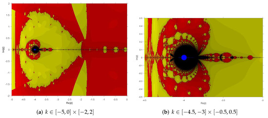
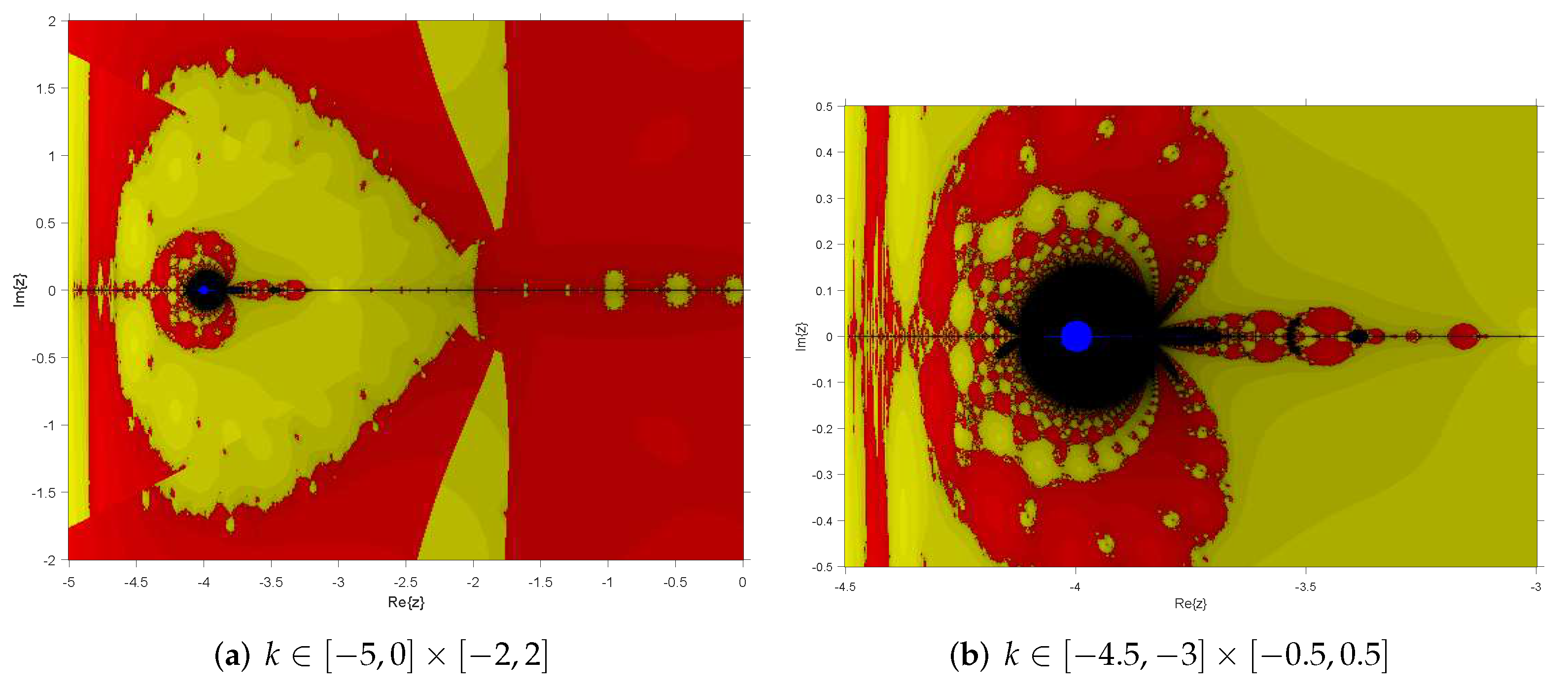
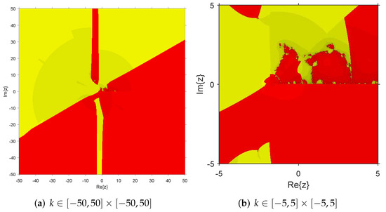
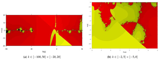
Now, we analyze the asymptotic behavior of the free critical points of our proposed method family (2) with the technique [13]. These free critical points that depend on k are the roots of polynomial $\chi \left(z\right)$. For this, we draw the parameter space related to points ${\eta }_j$. In the previous analysis, we already know that the free critical points are conjugated, so only three planes need to be drawn. We create a mesh of $500\times 500$ points in the complex plane and each point corresponds a different complex parameter value k. We select $z_0={\eta }_j\left(k\right)$ as an initial estimate for iterative schemes (2) where k goes through every point in the mesh and set the maximum number of iterations to 50. If the method converges to $z=1$, the points are painted in blue; red denotes the convergence of the method to 0 (associated with a); yellow denotes those points that eventually converge to ∞ (associated with the b) and they are black in other cases, i.e., they diverge.

The parameter space related to the free critical points ${\eta }_j$ are obtained in Figure 4, Figure 5, Figure 6 about different intervals. $k\in [a,b]\times [c,d]$ where $[a,b]$ and $[c,d]$ are the range of the real and imaginary parts of k, respectively; (b) is a detail on (a). In Figure 4b, we observe a small disk (the blue is denoted by D): D corresponds to values of k for which $z=1$ is attractive or superattractive. In addition, it is very clear that, except for the red and yellow areas, the other color domains are not the best for the selection of the parameter k-value in terms of stability. From Figure 4, Figure 5, Figure 6, we see broad regions for red and yellow, suggesting that some members of family (2) are numerically stable. We will analyze the dynamic plane of family (2) with parameter k in the red and yellow areas of Figure 4, Figure 5, Figure 6.

Figure 4. Parameter space associated with the free critical point ${\eta }_1$.

Figure 5. Parameter space associated with the free critical point ${\eta }_2$.

Figure 6. Parameter space associated with the free critical point ${\eta }_3$.

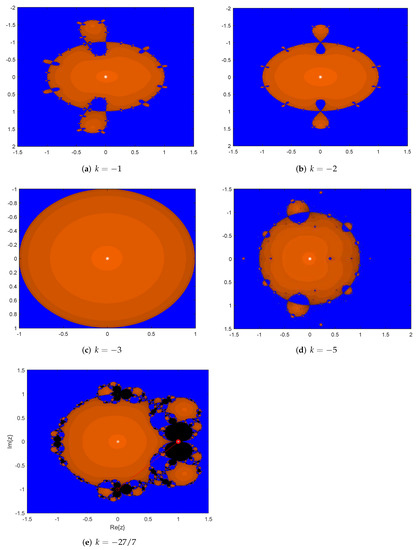
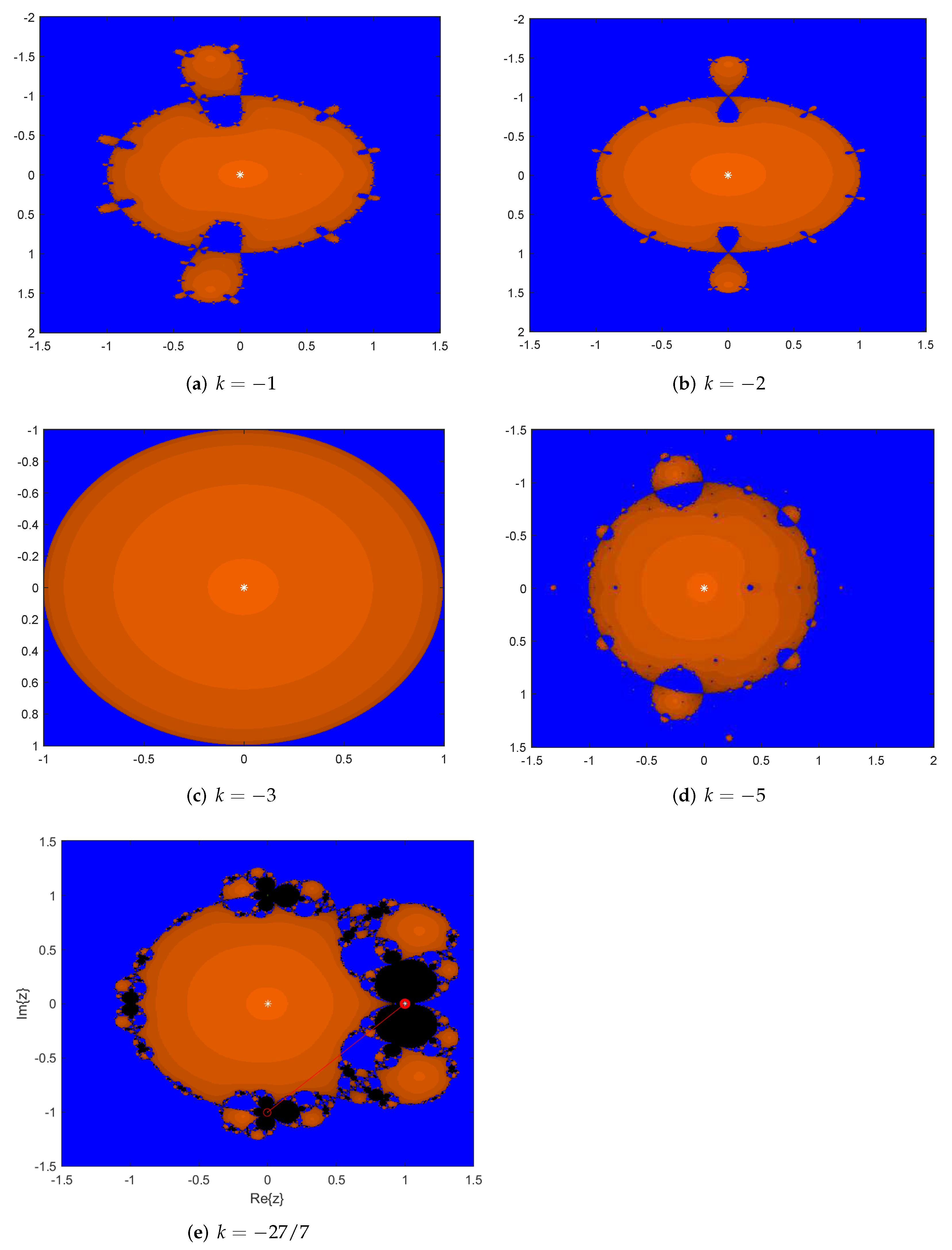
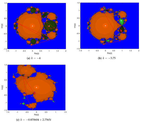
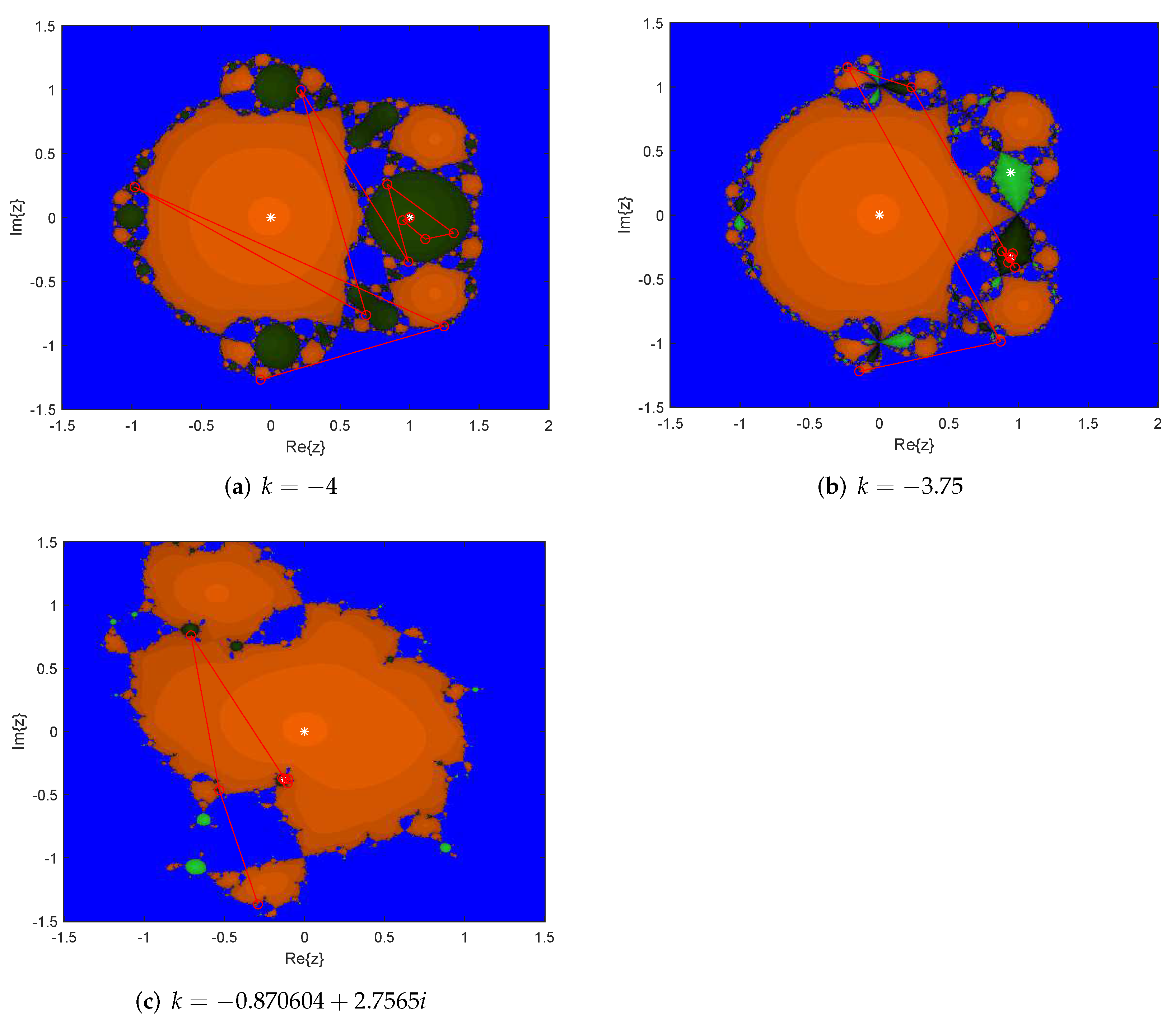
The dynamic plane of the new family (2) for a given value of k is presented. Each basin of attraction is painted in a different color: convergence to 0 and ∞ are in orange and blue, respectively; if it converges to the fixed point $z=1$ then it is in green; black indicates that the point does not converge to any root. We plotted the orbit of a point in red. Similarly to the parametric space, the maximum number of iterations is 50, and these dynamic planes are generated by a mesh of $500\times 500$ points.

First of all, we provide dynamical planes for $k=-1,k=-2,k=-3,k=-5$ and $k=-27/7$ in Figure 7, respectively. It can be seen that only the black color appears in Figure 7e. In addition to Figure 7e, the attraction basins in other planes are only related to a or b, which means that k-values have good convergence properties. In other words, the corresponding members of the Ostrowski-type iterative family (2) are numerically stable.

Figure 7. Dynamical planes for special k-values.

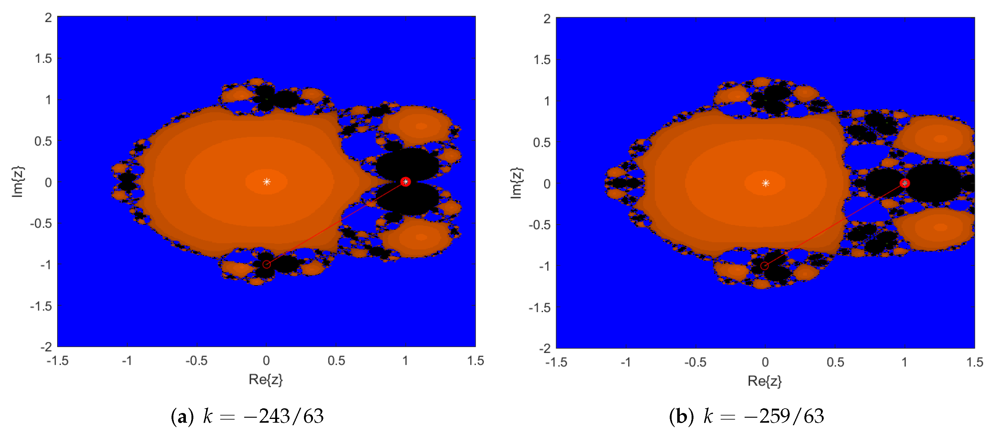
Figure 8 presents the dynamic planes converging to the strange fixed point for $k=-4,$$k=-3.75$ and $k=-0.870604+2.7565i$. Furthermore, three different basins of attraction appear in each figure.

Figure 8. Dynamical planes converging to the strange fixed points.

In Figure 9, different kinds of unstable behavior can be found. Figure 9 shows that $z=1$ is a parabolic fixed point which is consistent with Theorem 5(c) and then it exists in the Julia set but it has its own basin of attraction (black in the figure).

Figure 9. Dynamical planes for $|k+251/63|=8/63$.

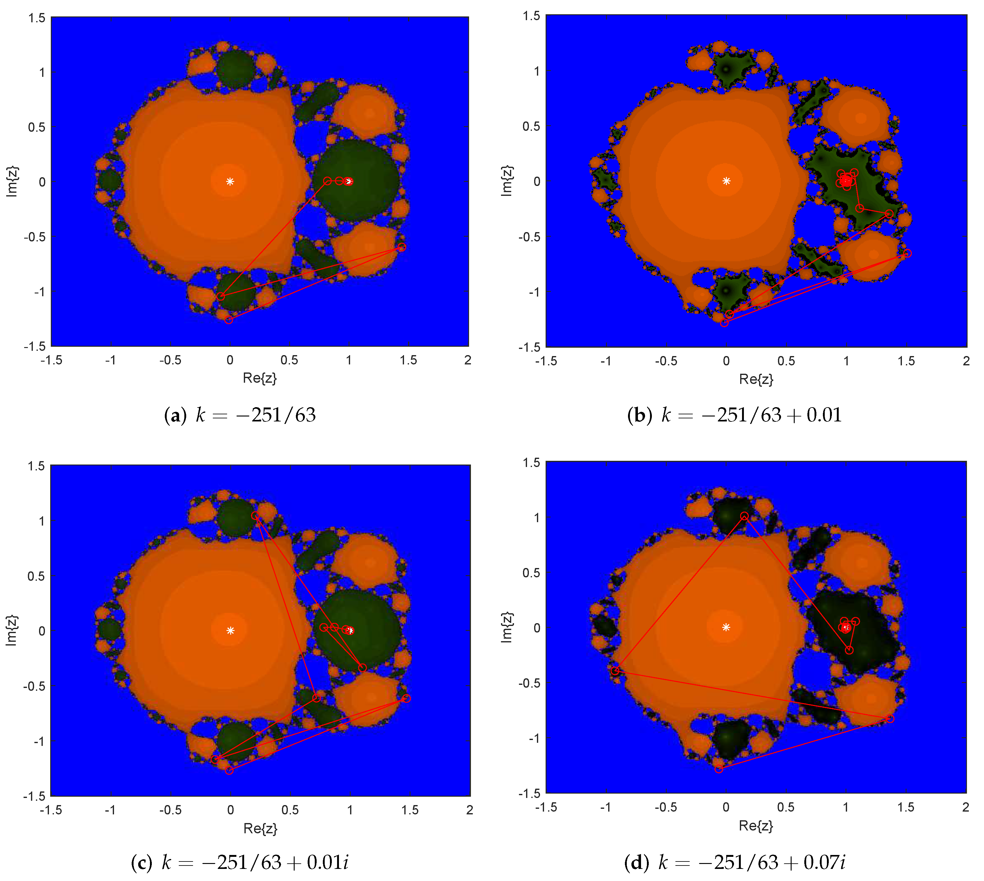
Finally, in Figure 10a, the dynamical plane of the iterative scheme corresponds to $k=-251/63$ (the center of circle S) is shown. Figure 10b–d are the dynamic planes with respect to the neighborhood of $-251/63$ but still within the circle S. We find that with $-0.01198-1.262i,-0.01896-1.283i,-0.01198-1.269i$ and $-0.06088-1.283i$ as the initial points, respectively, their orbits eventually converge to $z=1$, which corresponds to Theorem 5 (b) and Remark 2.

Figure 10. Dynamical planes of the neighborhood of $-251/63$.

Through the above analysis, we can see that these methods corresponding to $k=-1,k=-2,k=-3$ and $k=-5$ outperform the other elements of the Ostrowski-type iterative family (2) in most numerical applications. Furthermore, $t=1,k=-3$ is the most stable member due to Cayley’s test [17].

6. Numerical Experiments

In this section, different test functions and previous methods are used to verify the effectiveness of the proposed method OM. The iterative methods used are as follows.

Gupta et al. presented the method (GM, see [18]):

$$\left\{\begin{array}{c}{y}_n=x_n-\frac{f\left(x_n\right)}{f^{\prime }\left(x_n\right)},\hfill \\ w_n=y_n-\frac{f\left(y_n\right)}{f^{\prime }\left(x_n\right)}\frac{f\left(x_n\right)}{f\left(x_n\right)-2f\left(y_n\right)},\hfill \\ x_{n+1}=w_n-\frac{f\left(w_n\right)(w_n-y_n)}{f\left(w_n\right)-f\left(y_n\right)}.\hfill \end{array}\right.$$

(29)

Maroju et al. showed the method (MM, see [11]):

$$\left\{\begin{array}{c}{y}_n=x_n-\frac{f\left(x_n\right)}{f^{\prime }\left(x_n\right)},\hfill \\ z_n=x_n-\left(1+\frac{f\left(y_n\right)}{f\left(x_n\right)}\frac{f\left(x_n\right)+f\left(y_n\right)}{f\left(x_n\right)-f\left(y_n\right)}\right)·\frac{f\left(x_n\right)}{f^{\prime }\left(x_n\right)},\hfill \\ x_{n+1}=z_n-\frac{f\left(z_n\right)}{f^{\prime }\left(x_n\right)+g\left(x_n\right)(z_n-x_n)}.\hfill \end{array}\right.$$

(30)

where:

$$g\left(x_n\right)=\frac{2f\left(y_n\right){f^{\prime }\left(x_n\right)}^2}{{f\left(x_n\right)}^2}.$$

Table 3 shows the test functions used in the subsequent comparison. As seen in Table 4, we clearly know that the error of $k=-3$ is the smallest under the same number of iterations, which is the same as the result in the dynamic plane. As Table 5 suggests, our proposed method shows favorable performance compared to Maroju and Gupta methods.

Table 3. The function $f_i\left(x\right)$, initial guesses $x_0$ and zeros $\alpha$.

i	${\mathit{f}}_{\mathit{i}}\left(\mathit{x}\right)$	${\mathit{x}}_0$	$\mathit{\alpha }$
1	${sin}^2\left(x\right)-x^2+1$	1.3	1.4044916482153412
2	$x^3-10$	2	2.1544346900318837
3	$cos\left(\frac{\Pi }{2}x\right)+x^2-\Pi$	2	2.0347248962791266
4	${exp}^{x}sinx+log(x^2+1)$	1	0
5	$x^4-logx-5$	1.6	1.5259939537536892

Table 4. Comparison for special k-values.

k	${\mathit{f}}_{\mathit{i}}\left(\mathit{x}\right)$	$|{\mathit{x}}_1-{\mathit{x}}_0|$	$|{\mathit{x}}_2-{\mathit{x}}_1|$	$|{\mathit{x}}_3-{\mathit{x}}_2|$	$|{\mathit{x}}_4-{\mathit{x}}_3|$
−5	$f_1\left(x\right)$	0.10449	1.7367 × ${10}^{-6}$	2.8778 × ${10}^{-35}$	5.9578 × ${10}^{-208}$
	$f_2\left(x\right)$	0.15443	9.537 × ${10}^{-7}$	4.6831 × ${10}^{-38}$	6.5657 × ${10}^{-226}$
−1	$f_1\left(x\right)$	0.10449	2.0417 × ${10}^{-6}$	7.074 × ${10}^{-35}$	1.2239 × ${10}^{-205}$
	$f_2\left(x\right)$	0.15444	1.0177 × ${10}^{-6}$	5.8526 × ${10}^{-38}$	2.1164 × ${10}^{-225}$
−3	$f_1\left(x\right)$	0.10449	1.4665 × ${10}^{-7}$	3.5972 × ${10}^{-43}$	7.8344 × ${10}^{-257}$
	$f_2\left(x\right)$	0.15443	1.0231 × ${10}^{-7}$	5.4912 × ${10}^{-45}$	1.3126 × ${10}^{-268}$
−2	$f_1\left(x\right)$	0.10449	8.5343 × ${10}^{-7}$	1.8169 × ${10}^{-37}$	1.6918 × ${10}^{-221}$
	$f_2\left(x\right)$	0.15444	4.1677 × ${10}^{-7}$	1.2544 × ${10}^{-40}$	9.3276 × ${10}^{-242}$
−27/7	$f_1\left(x\right)$	0.10449	8.8583 × ${10}^{-7}$	2.272 × ${10}^{-37}$	6.467 × ${10}^{-221}$
	$f_2\left(x\right)$	0.15443	4.9404 × ${10}^{-7}$	4.2762 × ${10}^{-40}$	1.7983 × ${10}^{-238}$

Table 5. Comparison of iterative methods for the test functions.

${\mathit{f}}_{\mathit{i}}\left(\mathit{x}\right)$	n	OM		MM		OGM
		$|{\mathbf{x}}_{\mathbf{n}}-{\mathbf{x}}_{\mathbf{n}-\mathbf{1}}|$	$\left|\mathbf{f}\right({\mathbf{x}}_{\mathbf{n}}\left)\right|$	$|{\mathbf{x}}_{\mathbf{n}}-{\mathbf{x}}_{\mathbf{n}-\mathbf{1}}|$	$\left|\mathbf{f}\right({\mathbf{x}}_{\mathbf{n}}\left)\right|$	$|{\mathbf{x}}_{\mathbf{n}}-{\mathbf{x}}_{\mathbf{n}-\mathbf{1}}|$	$\left|\mathbf{f}\right({\mathbf{x}}_{\mathbf{n}}\left)\right|$
$f_1\left(x\right)$	1	1.0449 × ${10}^{-1}$	3.6406 × ${10}^{-7}$	1.0449 × ${10}^{-1}$	5.16692 × ${10}^{-7}$	1.0449 × ${10}^{-1}$	1.17938 × ${10}^{-6}$
	2	1.4665 × ${10}^{-7}$	8.9299 × ${10}^{-43}$	2.0814 × ${10}^{-7}$	2.43255 × ${10}^{-41}$	4.7508 × ${10}^{-7}$	7.22718 × ${10}^{-39}$
	3	3.5972 × ${10}^{-43}$	1.94486 × ${10}^{-256}$	9.7989 × ${10}^{-42}$	2.64877 × ${10}^{-247}$	2.9113 × ${10}^{-39}$	3.82701 × ${10}^{-232}$
	4	7.8344 × ${10}^{-257}$	2.07559 × ${10}^{-1538}$	1.067 × ${10}^{-247}$	4.41503 × ${10}^{-1483}$	1.5416 × ${10}^{-232}$	8.43734 × ${10}^{-1392}$
$f_2\left(x\right)$	1	1.5443 × ${10}^{-1}$	1.42466 × ${10}^{-6}$	1.5443 × ${10}^{-1}$	3.95386 × ${10}^{-6}$	1.5443 × ${10}^{-1}$	3.53539 × ${10}^{-6}$
	2	1.0231 × ${10}^{-7}$	7.6464 × ${10}^{-44}$	2.8394 × ${10}^{-7}$	1.39756 × ${10}^{-40}$	2.5389 × ${10}^{-7}$	5.35701 × ${10}^{-41}$
	3	5.4912 × ${10}^{-45}$	1.82778 × ${10}^{-267}$	1.0037 × ${10}^{-41}$	2.72565 × ${10}^{-247}$	3.8471 × ${10}^{-42}$	6.48392 × ${10}^{-250}$
	4	1.3126 × ${10}^{-268}$	3.4098 × ${10}^{-1609}$	1.9574 × ${10}^{-248}$	1.49989 × ${10}^{-1487}$	4.6564 × ${10}^{-251}$	2.03858 × ${10}^{-1503}$
$f_3\left(x\right)$	1	3.4725 × ${10}^{-2}$	9.21225 × ${10}^{-12}$	3.4725 × ${10}^{-2}$	1.68613 × ${10}^{-11}$	3.4725 × ${10}^{-2}$	3.70924 × ${10}^{-10}$
	2	2.2171 × ${10}^{-12}$	6.67277 × ${10}^{-73}$	4.058 × ${10}^{-12}$	7.38308 × ${10}^{-71}$	8.927 × ${10}^{-11}$	9.67886 × ${10}^{-62}$
	3	1.6059 × ${10}^{-73}$	9.63714 × ${10}^{-440}$	1.7769 × ${10}^{-71}$	5.20373 × ${10}^{-427}$	2.3294 × ${10}^{-62}$	3.05532 × ${10}^{-371}$
	4	2.3194 × ${10}^{-440}$	8.74583 × ${10}^{-2641}$	1.2524 × ${10}^{-427}$	6.3794 × ${10}^{-2564}$	7.3532 × ${10}^{-372}$	3.02312 × ${10}^{-2228}$
$f_4\left(x\right)$	1	0.95175	5.29461 × ${10}^{-2}$	0.95137	5.33921 × ${10}^{-2}$	0.95264	5.18821 × ${10}^{-2}$
	2	4.8254 × ${10}^{-2}$	1.67183 × ${10}^{-8}$	4.8627 × ${10}^{-2}$	4.89593 × ${10}^{-8}$	4.7363 × ${10}^{-2}$	2.02955 × ${10}^{-7}$
	3	1.6718 × ${10}^{-8}$	5.33748 × ${10}^{-47}$	4.8959 × ${10}^{-8}$	1.0712 × ${10}^{-43}$	2.0296 × ${10}^{-7}$	2.05003 × ${10}^{-39}$
	4	5.3375 × ${10}^{-47}$	5.65194 × ${10}^{-278}$	1.0712 × ${10}^{-43}$	1.17509 × ${10}^{-257}$	2.05 × ${10}^{-39}$	2.17731 × ${10}^{-231}$
$f_5\left(x\right)$	1	0.74006 × ${10}^{-1}$	4.74263 × ${10}^{-7}$	0.74006 × ${10}^{-1}$	2.48963 × ${10}^{-6}$	0.074006	1.29563 × ${10}^{-6}$
	2	3.4978 × ${10}^{-8}$	7.50338 × ${10}^{-45}$	1.8362 × ${10}^{-7}$	6.84712 × ${10}^{-40}$	9.5557 × ${10}^{-8}$	7.70349 × ${10}^{-42}$
	3	5.534 × ${10}^{-46}$	1.17674 × ${10}^{-271}$	5.05 × ${10}^{-41}$	2.96314 × ${10}^{-241}$	5.6816 × ${10}^{-43}$	3.40343 × ${10}^{-253}$
	4	8.6788 × ${10}^{-273}$	1.7507 × ${10}^{-1632}$	2.1854 × ${10}^{-242}$	1.94632 × ${10}^{-1449}$	2.5101 × ${10}^{-254}$	2.53102 × ${10}^{-1521}$

7. Conclusions

We analyze the stability of the Ostrowski-type iterative method with six orders. The dynamic analysis of any quadratic polynomial was performed to select the family members with better stability characteristics. The stability of the strange fixed points is studied. There are many possible values for which members of this family have been proven to have good stability from the parameter space. The dynamic plane also shows that some members of this family are numerically stable. The results in Figure 7 and Table 4 are consistent, that is, $t=1,k=-3$ has the best numerical behavior. Some numerical experiments support that the new method for $t=1,k=-3$ has better performance than existing methods.

References

- Ortega, J.M.; Rheinbolt, W.C. Iterative Solution of Nonlinear Equations in Several Variables; Academic Press: New York, NY, USA, 1970. [Google Scholar]
- Wang, X. A family of Newton-type iterative methods using some special self-accelerating parameters. Int. J. Comput. Math. 2017, 95, 2112–2127. [Google Scholar] [CrossRef] [Scilit]
- Wang, X. An Ostrowski-type method with memory using a novel self-accelerating parameter. J. Comput. Appl. Math. 2017, 330, 710–720. [Google Scholar] [CrossRef] [Scilit]
- Geaum, Y.H.; Kim, Y.I. Long-term orbit dynamics viewed through the yellow main component in the parameter space of a family of optimal fourth-order multiple-root finders. Discret. Contin. Dyn. Syst. Ser. B 2020, 25, 3087. [Google Scholar]
- Ostrowski, A.M. Solution of Equations in Euclidean and Banach Space; Academic Press: New York, NY, USA, 1973. [Google Scholar]
- Cordero, A.; Guasp, L.; Torregrosa, J.R. Choosing the most stable members of Kou’s family of iterative methods. J. Comput. Appl. Math. 2018, 330, 759–769. [Google Scholar] [CrossRef] [Scilit]
- Chun, C.; Ham, Y.M. Some sixth-order variants of Ostrowski root-finding methods. Appl. Math. Comput. 2007, 193, 389–394. [Google Scholar] [CrossRef] [Scilit]
- Blanchard, P. Complex analytic dynamics on the Riemann sphere. Bull. Amer. Math. Soc. 1984, 11, 85–141. [Google Scholar] [CrossRef] [Scilit]
- Carleson, L.; Gamelin, T.W. Complex Dynamics; Springer: New York, NY, USA, 1993. [Google Scholar]
- Thompson, J.M.T.; Stewart, H.B. Nonlinear Dynamics and Chaos; John Wieley and Sons Ltd.: New York, NY, USA, 1986. [Google Scholar]
- Maroju, P.; Magrenan, A.A.; Mosta, S.S.; Sarria, I. Second derivative free sixth order continuation method for solving nonlinear equations with applications. J. Math. Chem. 2018, 56, 2099–2116. [Google Scholar] [CrossRef] [Scilit]
- Magreñán, Á.A. Different anomalies in a Jarratt family of iterative root-finding methods. Appl. Math. Comput. 2014, 233, 29–38. [Google Scholar]
- Chicharro, F.I.; Cordero, A.; Torregrosa, J.R. Drawing dynamical and parameters planes of iterative families and methods. Sci. World J. 2013, 2013, 780153. [Google Scholar] [CrossRef] [Scilit] [PubMed]
- Ahlfors, L.V. Complex Analysis; McGraw-Hill Book, Inc.: New York, NY, USA, 1979. [Google Scholar]
- Beardon, A.F. Iteration of Rational Function; Springer: New York, NY, USA, 1991. [Google Scholar]
- Wolfram, S. The Mathematica Book, 5th ed.; Wolfram Media: Champaign, IL, USA, 2003. [Google Scholar]
- Babajee, D.K.R.; Cordero, A.; Torregrosa, J.R. Torregrosa, Study of multipoint iterative methods through the Cayley Quadratic Test. J. Comput. Appl. Math. 2014, 291, 358–369. [Google Scholar] [CrossRef] [Scilit]
- Parhi, S.K.; Gupta, D.K. A sixth order method for nonlinear equations. Appl. Math. Comput. 2012, 218, 10548–10556. [Google Scholar] [CrossRef] [Scilit]
Publisher’s Note: MDPI stays neutral with regard to jurisdictional claims in published maps and institutional affiliations. |
© 2022 by the authors. Licensee MDPI, Basel, Switzerland. This article is an open access article distributed under the terms and conditions of the Creative Commons Attribution (CC BY) license (https://creativecommons.org/licenses/by/4.0/).