Article

Mixed Convection Flow over an Elastic, Porous Surface with Viscous Dissipation: A Robust Spectral Computational Approach

by
Lijun Zhang
1,2,
Nafisa Tariq
1,
Muhammad Mubashir Bhatti
1,* and
Efstathios E. Michaelides
3
1
College of Mathematics and Systems Science, Shandong University of Science and Technology, Qingdao 266590, China
2
International Institute for Symmetry Analysis and Mathematical Modelling, Department of Mathematical Sciences, North-West University, Mafikeng Campus, Mmabatho 2735, South Africa
3
Department of Engineering, Texas Christian University, Fort Worth, TX 76132, USA
*
Author to whom correspondence should be addressed.
Fractal Fract. 2022, 6(5), 263; https://doi.org/10.3390/fractalfract6050263
Submission received: 11 April 2022 / Revised: 6 May 2022 / Accepted: 7 May 2022 / Published: 10 May 2022

Abstract

:
A novel computational approach is developed to investigate the mixed convection, boundary layer flow over a nonlinear elastic (stretching or shrinking) surface. The viscous fluid is electrically conducting, incompressible, and propagating through a porous medium. The consequences of viscous dissipation, Joule heating, and heat sink/source of the volumetric rate of heat generation are also included in the energy balance equation. In order to formulate the mathematical modeling, a similarity analysis is performed. The numerical solution of nonlinear differential equations is accomplished through the use of a robust computational approach, which is identified as the Spectral Local Linearization Method (SLLM). The computational findings reported in this study show that, in addition to being simple to establish and numerically implement, the proposed method is very reliable in that it converges rapidly to achieve a specified goal and is more effective in resolving very complex models of nonlinear boundary value problems. In order to ensure the convergence of the proposed SLLM method, the Gauss–Seidel approach is used. The SLLM’s reliability and numerical stability can be optimized even more using Gauss–Seidel approach. The computational results for different emerging parameters are computed to show the behavior of velocity profile, skin friction coefficient, temperature profile, and Nusselt number. To evaluate the accuracy and the convergence of the obtained results, a comparison between the proposed approach and the bvp4c (built-in command in Matlab) method is presented. The Matlab software, which is used to generate machine time for executing the SLLM code, is also displayed in a table.

1. Introduction

Heat transfer over an elastic surface has attracted the interest of researchers around the globe because of its numerous applications in manufacturing and commercial processes such as glass blowing, polymer extrusion, hot rolling, metal spinning, and wire drawing [1,2]. Many chemical engineering processes [3,4], such as metallurgical operations and polymer extrusion processes involve the cooling of a molten liquid that is stretched into a cooling system, have made use of the momentum and heat transfer of boundary layer flow across the stretching surface. In these applications, continuous strips of filaments are cooled by drawing them through a quiescent fluid. The process of drawing stretches the filaments. Rahmati et al. [5] investigated the non-Newtonian nanofluid flow under the impact of no-slip and slip conditions. Sene [6] discussed the effects of Newtonian heating using a second-grade fluid with Caputo fractional derivative.
The heat transfer process through porous media is applicable in a variety of fields ranging from Ceramic Engineering to Geophysiscs as it appears below in Table 1.
All of these applications provide an incentive to further investigate the mixed convection flow in a porous medium with a non-linear elastic surface.
Among the previous studies on the subject, Sakiadis [14] investigated the behavior of the boundary layer on a continuous, stable subsurface, including both laminar and turbulent flow. Crane [15] further extended the work of Sakiadis and investigated a Newtonian fluid induced by a linearly stretched flat surface. He derived an exact solution for the problem in closed form. More recently, Rosca and Pop [16] examined the heat transfer across a stretching/shrinking sheet using a second order slip flow model. They used the Matlab’s bvp4c function for their numerical solutions. The effect of a heat source/sink on a viscous fluid passing through a porous medium was studied by Swain et al. [17]. Othman et al. [18] used the shooting method, which generates numerical solutions for the stagnation point of a steady 2-D mixed convection flow across a stretching/shrinking surface. Kumar et al. [19] also explored the role of Joule heating on the thermal boundary layer flow and heat transfer over a stretching surface. The effects of buoyancy on the two-dimensional mixed convection and Casson fluid along a linearly stretching sheet was studied by Gangadhar et al. [20]. Their numerical solutions were obtained by a spectral relaxation analysis. Prabha et al. [21] used the LTNE model to evaluate the 2-D mixed convection boundary layer flow through a porous medium. Badruddin et al. [22] provided a brief overview of heat transfer through porous materials. Ali et al. [23] examined the flow over a stretching sheet with a porous surface. Ilya et al. [24] used a Finite-Difference approach to investigate the occurrence of mixed convection flow along the surface of a cone immersed in a porous medium in the presence of a heat source/sink, a magnetic field, and density difference that induce buoyancy. Adeniyan et al. [25] studied the similarity solutions within the context of convective boundary layer flow and heat transfer around a stretching hollow cylinder, immersed and filled with a viscoelastic fluid. To obtain numerical results, they used the Runge–Kutta–Fehlberg integration method together with the shooting method.
Viscous dissipation is important in many areas: significant temperature rises have been experimentally observed in polymer processes, such as fast extrusion or injection molding. Aerodynamic heating in a thin boundary layer around high-speed rail and aircraft elevates their surface temperature. In a completely different application, the dissipation function is used to express the viscosity of dilute suspensions [26]. Viscous dissipation is also observed in convection mechanisms [27,28,29] for various devices that are operate at high relative velocities or at high rotational velocities. The impact of viscous dissipation can be also seen in planetary processes because it causes stronger gravitational fields with large masses of gas and larger planets.
The field of magnetohydrodynamics (MHD) flow and heat transfer has applications in a wide range of industries, ecological systems, and geophysical explorations. For example, paper manufacturing, glass-fiber manufacturing, and the fabrication of polymer sheets from dies, continuous casting and wire drawing are all examples of industrial processes related to this field. Because of their industrial applications, such flows have been addressed by a variety of researchers, including: Jafar et al. [30] evaluated the steady boundary layer flow of incompressible and viscous fluids under the effects of MHD. Dessie et al. [31] studied the relationship of viscous dissipation as a heat source/sink in MHD flow and heat transfer via porous media across a stretched sheet. The solutions of the governing equations in this study were calculated by employing Lie’s group transformations. Bibi et al. [32] used the shooting technique to numerically investigate the unsteady MHD flow of a Williamson fluid with heat transfer on a pervious stretchable sheet. Alarifi et al. [33] numerically assessed the MHD boundary layer flow over a vertical stretched surface, in the presence of a heat source/sink and a magnetic force. They used the RKFI approach to identify numerical solutions to the nonlinear differential equations. Also, Swain et al. [34] explored the effects of Joule heating and viscous dissipation on MHD flow and heat transfer via porous material. Megahed et al. [35] described an unsteady magnetized fluid flow with thermal radiation effects and heat flux conditions. To obtain numerical solutions, they combined the shooting method with a Runge–Kutta algorithm. Sarda et al. [36] considered a non-Newtonian fluid propagating over a stretching surface and non-equilibrium thermal conditions to investigate the effect of magnetic fields on heat transfer. They also used a combination of shooting technique and the fourth-fifth-order Runge–Kutta–Fehlberg (RKF) method. Zhou et al. [37] examined the role of slip on a stretchable surface with a non-uniform heat source using Casson fluid. They used the bvp4c command to develop solutions to the nonlinear problem. Ullah et al. [38] used a new stochastic method to investigate the MHD boundary layer flow. Recently, Bhatti et al. [39] used a Lie group analysis and a successive linearization technique to solve a nonlinear Jeffrey fluid model with mass transport.
The primary goal of this paper is to present a rigorous computational method for solving nonlinear boundary value problems. The proposed methodology is a simple, precise, and convergent algorithm and is known as the spectral local linearization method, abbreviated as SLLM. This method involves linearizing and decoupling equations using a univariate linearization approach and spectral collocation linearization. The proposed algorithm’s main distinguishing feature is that it converts a large coupled system of equations into a set of smaller systems that can be solved sequentially in a computationally efficient manner. We applied this methodology to a nonlinear problem, such as two coupled nonlinear differential equations of mixed convection heat transfer. The results show that, when compared to other similar methods, the computed methodology is simple to develop, fast converging, efficient, accurate, and reliable.
Not enough emphasis has been given to the mixed convection fluid flow with viscous dissipation. The majority of the literature reported above used the bvp4c, a shooting method, the Runge–Kutta approach or other numerical and analytical techniques to solve nonlinear boundary layer flow problems. Spectral numerical methods, like SLLM, were not used to solve such problems. The primary goal of this research is to use a robust computational technique to assess the mixed convection fluid flow including magnetic and porous effects. The energy equation takes into account the simultaneous effects of viscous dissipation, heat source/sink, and Joule heating. Following a similarity analysis, the numerical solutions to the governing equations were obtained using the computational approach of Spectral Local Linearization. The Gauss–Seidel technique is also used to improve the convergence of this method. The suggested methodology’s machine time is also given in tabular form utilizing the Matlab software. Full numerical and graphical comparisons with the bvp4c [40] and previously reported studies are also provided in this paper.

2. Problem Description and Modeling

We consider a two-dimensional mixed convective flow of a viscous incompressible fluid induced by a nonlinear elastic sheet, while stretching or shrinking, with a porous medium. The flow is modeled in a Cartesian coordinate system, with the x -coordinate along the moving surface and the y -coordinate in the normal to the surface direction. The elastic sheet is at rest on the plane y = 0 , which also incorporates the heat sink/source with volumetric heat absorption or generation Q 0 = x q 0 (where q 0 is constant). The nonlinear elastic sheet is deformed with a wall velocity w s ( x ) = c x 2 , where the constant parameter c is positive during stretching ( c > 0 ) and negative during shrinking ( c < 0 ) . The elastic surface is permeable. The process is an injection when the velocity is v s < 0 and suction when the velocity is v s > 0 . The fluid is electricity conducting when exposed to the influence of a uniform variable magnetic field B 0 = b 0 x and traveling through a porous material with variable permeability k = k 0 / x . Furthermore, T w signifies temperature at the wall, while T inf indicates the ambient temperature distant from the surface. The governing equations for this physical problem are formulated using the standard boundary layer approximations [41]:
u x + v y = 0 ,
u u x + v u y = ν 2 u y 2 + d g χ T T inf σ B 0 2 ρ u ν k u ,
where u and v represent the velocity components in x - and y - coordinates, ρ denotes the density, ν denotes the kinematic viscosity, g is the gravitational acceleration, χ denotes the coefficient of the thermal expansion, μ is the fluid viscosity, σ denotes the electrical conductivity, and d is a dummy parameter with values 0 , + 1 or 1 .
u T x + v T y = α 2 T y 2 + Q 0 ρ c p T T inf + V . D . ,
where α denotes the thermal diffusivity, c p denotes the specific heat capacity, and V.D. is the viscous dissipation, defined as follows:
V . D . = 1 ρ c p μ u y 2 + σ B 0 2 u 2 + μ k u 2 .
The boundary conditions at y = 0 are defined as:
u = w s x = c x 2 , v = x 1 2 v s , T = T w x = T inf + b x 3 ,
where b is a constant that indicates a hot plate when b > 0 and a cool plate when b < 0 .
The boundary conditions at y are defined as:
u 0 , u y 0 , T T inf .

Similarity Analysis

The following transformations are introduced for the solution of the governing equations:
η = y 3 | c | x 2 ν , u = | c | x 2 f η , v = 1 2 2 3 ν | c | x 3 f η + η f η , T = b x 3 θ + T inf ,
and the velocity of the wall mass transfer becomes v s = 3 ν | c | 2 ς . Applying Equation (7) to the governing Equations (2)–(6), we derive the following set of differential equations
f + f f 4 3 f 2 ( β + γ ) f + Λ θ = 0 ,
θ + Γ f θ 2 f θ + λ f 2 + λ ( β + γ ) f 2 + δ θ = 0 ,
where β = 2 σ b 0 2 3 | c | ρ denotes the magnetic parameter, γ = 2 υ 3 k 0 | c | denotes the permeability parameter, λ = w s 2 c p ( T w T inf ) denotes the Eckert number, Γ = ν α denotes the Prandtl number, δ = 2 3 q 0 ρ c p | c | denotes the local heat generation/absorption coefficient, Λ = d 2 3 G r 2 denotes the mixed convention parameter, G r = g χ ( T w T inf ) x 3 υ 2 denotes the Grashof number, and = w s x υ denotes the Reynolds number. Mixed convection occurs when the mechanisms of forced and natural convection work in tandem to transfer heat. The Grashof number (for natural convection) and the Reynolds number (for forced convection) are two dimensionless numbers that are frequently used to define the strength of each part of the convection [42,43].
The boundary conditions reduce to the following form:
f 0 = ς , f 0 = ϕ , θ 0 = 1 , f = 0 , θ = 0 ,
where ς denotes the wall transpiration, and ϕ is the stretching/shrinking parameter. If ϕ > 0 the surface is stretching and if ϕ < 0 the surface shrinks.
The skin friction coefficient and the Nusselt number are expressed as follows:
C f = τ s ρ w s 2 u y y = 0 , N u = x q f κ T w T inf ,
where κ represents the thermal conductivity. The wall shear stress τ s , and the surface heat flux q f are given by the equations:
τ s = μ u y y = 0 , q f = κ T y y = 0 .
Using Equations (7) and (11), we obtain the following expressions:
1 2 C f = 3 2 f 0 , 1 2 N u = 3 2 θ 0 .
It can be seen that the resulting Equations (8) and (9) are nonlinear and coupled. Exact and closed-form solutions to these differential equations are impossible to derive. Therefore, in the following section, we will present a robust computational method to solve the system of equations.

3. Implementation of Numerical Method

3.1. Basic Steps to Apply Spectral Local Linearization Method

Let us consider a system of differential equations F = f 1 ( η ) , f 2 ( η ) , , f m ( η ) that fulfill the condition:
L n + N n = H n , n = 1 , 2 , , m ,
where m denotes the number of differential equations. Each H n is a function of η A , B , and L n , N n represent the system’s linear and nonlinear components, respectively.
To continue the iteration process, the local linearization of N n at approximately F n , t (latest iteration) is employed for the nth nonlinear equation by assuming that all other F l , t ( l n ) values are known.
N n f 1 ( η ) , f 2 ( η ) , , f m ( η ) = N n f 1 , t , f 2 , t , , f m , t + N n f 1 , t , f 2 , t , , f m , t ( f n f n , t ) .
As a result, for the current iteration with f n = f n , t + 1 , Equation (14) becomes
L n f 1 , t , f 2 , t , f m , t + 1 + N n f 1 , t , f 2 , t , , f m , t f 1 , t + 1 = H n + N n f 1 , t , f 2 , t , , f m , t f 1 , t N n f 1 , t , f 2 , t , , f m , t ,
L m f 1 , t , f 2 , t , , f m , t + 1 + N m f 1 , t , f 2 , t , , f m , t f m , t + 1 = H m + N m f 1 , t , f 2 , t , , f m , t f m , t N m f 1 , t , f 2 , t , , f m , t ,
where the nth equation f 1 , t , f 2 , t , , f m , t f 1 , t + 1 , f 2 , t + 1 , , f n 1 , t + 1 , f n , t , , f m , t .
Traditionally, the SLLM is an iterative procedure for solving differential equations that begins with an initial approximation f 0 and then is implemented iteratively, generating new approximations f 1 , f 2 , f 3 , , where F t = [ f 1 , t , f 2 , t , f m , t ] for each t = 0 , 1 , 2 , . Once the nonlinear components N n have been linearized, Equations (16) and (17) can be numerically solved utilizing the Chebyshev spectral collocation approach.
The nth differential Equation (14) after the first t + 1 iterations can be expressed in this manner:
L n + 1 + N n + 1 = H n .
Taylor series can be used to linearize the nonlinear components. For instance
N n | t + 1 = N n | t + N n | t V t + 1 V t ,
where V t denotes the n-tuples of F n , t and its differentials.
It is now possible to use Equations (18) and (19) into Equation (14) to obtain
L n | t + 1 + N n | t V t + 1 = H n + N n | t V t N n | t .

3.2. Implementation of the Spectral Local Linearization Method

To develop the SLLM, the current system of differential equations must be reduced in order, hence, we assume that f = h , to obtain the transformed Equations (8) and (9) in the form:
h + f h β + γ h 4 3 h 2 + Λ θ = 0 ,
θ + Γ f θ 2 h θ + λ h 2 + λ β + γ h 2 + δ θ .
We linearized the non-linear term h 2 using a Taylor series expansion, which is described in more detail below:
h t + 1 2 = 2 h t h t + 1 h t + h t 2 = 2 h t + 1 h t h t 2 ,
where the component with the subscript t + 1 represents the current approximated value and the component with the subscript t represents the previous value. Equation (23) is substituted in Equation (21), and the nonlinear system is decoupled by applying the Gauss–Seidel relaxation method to obtain the desired result. Thus, we have:
f t + 1 = h t ,
h t + 1 + f t h t + 1 β + γ h t + 1 8 3 h t h t + 1 = 4 3 h t 2 Λ θ t ,
θ t + 1 + Γ [ f t θ t + 1 2 h t + 1 θ t + 1 + δ θ t + 1 ] = λ h t + 1 2 + β + γ h t + 1 2 .
The pertinent boundary conditions are transformed as follows:
f t + 1 0 = ς , h t + 1 0 = ϕ , θ t + 1 0 = 1 ,
h t + 1 = 0 , θ t + 1 = 0 .
We write Equations (24)–(26) in a concise form as:
f t + 1 = E 00 ,
h t + 1 + E 11 h t + 1 E 13 h t + 1 E 12 h t + 1 = E 1 , t ,
θ t + 1 + Γ E 11 θ t + 1 2 h t + 1 θ t + 1 + δ θ t + 1 = E 2 , t ,
where
E 00 = h t , E 11 = f t , E 12 = 8 3 h t , E 13 = β + γ , E 1 , t = 4 3 h t 2 Λ θ t , E 2 , t = λ h t + 1 2 + β + γ h t + 1 2 .
Now, we apply the Chebyshev spectral collocation method to the system of Equations (24)–(26), where the differentiation matrix [44] D = 2 l D is used to approximate the derivatives of the unknown variables in the above equations. The physical region of the problem [ 0 , ) is truncated to [ 0 , l ] to allow the numerical implementation using the spectral technique, where l is stipulated to be sufficiently high. Our new system is written as:
D f t + 1 = h t ,
{ D 2 + diag [ E 11 ] D E 13 I E 12 I } h t + 1 = E 1 , t ,
{ D 2 + Γ diag [ E 11 ] D 2 diag [ h t + 1 ] + δ I } θ t + 1 = E 2 , t .
The corresponding boundary conditions are:
f t + 1 η N = ς , h t + 1 η N = ϕ , θ t + 1 η N = 1 ,
h t + 1 η 0 = 0 , θ t + 1 η 0 = 0 .
This system of equations may be expressed in a more concise form as follows:
B 1 f t + 1 = C 1 ,
B 2 h t + 1 = C 2 ,
B 3 θ t + 1 = C 3 ,
where
B 1 = D , C 1 = h t ,
B 2 = D 2 + diag [ E 11 ] D E 13 I E 12 I , C 2 = E 1 , t ,
B 3 = D 2 + Γ diag [ E 11 ] D 2 diag [ h t + 1 ] + δ I , C 3 = D 2 , t ,
where the diagonal matrices “diag” are defined as follows:
diag [ E 11 ] = E 11 ( η 0 ) . . E 11 ( η N ) , diag [ E 12 ] = E 12 ( η 0 ) . . E 12 ( η N ) ,
diag [ E 1 , t ] = E 1 , t ( η 0 ) E 1 , t ( η N ) , diag [ E 2 , t ] = E 2 , t ( η 0 ) E 2 , t ( η N ) ,
and
f t + 1 = [ f η 0 , f η 1 , , f η N ] T ,
h t + 1 = [ h η 0 , h η 1 , , h η N ] T ,
θ t + 1 = [ θ η 0 , θ η 1 , , η N ] T ,
where I represents the identity matrix of order N + 1 × N + 1 . Equations (46)–(48) represents the vectors of size N × 1 × 1 .
In light of Equation (10), the following initial guesses are chosen for the implementation of the method:
f 0 η 0 = ς + ϕ 1 exp [ η ] , h 0 η 0 = ϕ exp [ η ] , θ 0 η 0 = exp [ η ] .
These initial stipulations are used to obtain further approximations of f t , h t , θ t for each t = 1 , 2 , 3 , by using the suggested technique.

3.3. Convergence Analysis

The Gauss–Seidel technique with successive over relaxation parameter is often used to accelerate the convergence of the linear system of equations. In this case, an equivalent approach is utilized to accelerate the convergence rate for SLLM. At the ( t + 1 ) th iteration, the SLLM approach is used to solve the function Z .
B 1 Z t + 1 = C 1 .
The new mode of the SLLM approach is then represented by rewriting the equation as:
B 1 Z t + 1 = 1 Ω B 1 Z t + Ω C 1 .
Here Ω denotes the convergence parameter. If the value of Ω is between 1 and 2, the current value has a higher weight than the prior value. The current value must also be close to the old value. This procedure will help to improve the convergent system even more. This form of change is known as over relaxation, and the process is known as the SOR approach (successive over relaxation). The improved SLLM approach significantly contributes to the improvement of the accuracy and numerical efficiency.

4. Numerical Results and Discussion

The numerical solution for the velocity profile, the skin friction coefficient, the Nusselt number, and the temperature profile are discussed in this section. The Matlab software is used to plot all of the numerical results graphically. We chose the appropriate parametric values for the graphical results such as: N = 100 , β = 0.2 , γ = 0.2 , δ = 0.1 , Γ = 1 , Λ = 0.1 , λ = 0.5 , ς = 0 , ϕ = 1 . Table 2 shows the machine time (s), which indicates the execution time of numerical coding in Matlab. Table 3 shows the effect of N on the skin friction coefficient and the Nusselt number. This table indicates that the desired level of accuracy (up to five decimal places) can be obtained when N = 100 with four iterations. In addition, Table 4 and Table 5 illustrate the numerical results for the Skin friction and Nusselt number profile as functions of the adjustable parameters. We have also included a comparison with the bvp4c (built-in command in Matlab) in both tables (Table 4 and Table 5). We observe in these Tables that the results obtained by the two methods agree very well, indicating that the current approach, the SLLM, has been appropriately implemented. The data shows that the magnetic parameter β , the permeability parameter γ , the wall transpiration parameter ς , the shrinking or stretching parameter ϕ , and the Prandtl number Γ cause the skin friction profile to reduce. On the contrary, the mixed convection parameter Λ , the heat source or sink parameter δ , and the Eckert number λ augment the skin friction profile. The Nusselt number increases significantly because of the effect of the mixed convective parameter Λ and the Prandlt number Γ , whereas the magnetic parameter β , the permeability parameter γ , the Eckert number λ , and the heat source/sink δ tend to reduce the Nusselt number. Furthermore, Table 6 shows a numerical comparison of the skin friction profile with previously published data for β = 0 , γ = 0 , Λ = 0 , ς = 1 / 6 , ϕ = 1 . It is clear from this table that the current results are compatible with the previous studies.
Figure 1 and Figure 2 provide a graphical comparison of the velocity and temperature profiles. The solid line depicts the results of SLLM, whereas the red circle depicts the results of bvp4c. Matlab software is used to implement both solutions. The bvp4c (built-in command) is based on the shooting method. We can observe from these data that the two graphical outcomes agree well.
Figure 3 demonstrates the impact of the magnetic parameter β on the velocity profile. It is evident in this Figure that the velocity profile diminishes as the magnetic parameter increases. Because electromagnetic forces are proportional to magnetic fields, boosting the magnetic parameter increases the electromagnetic force, and this restricts the fluid motion over the whole surface. The temperature profile was significantly improved by increasing the parameter β , as shown in Figure 4. The Lorentz force opposes the fluid motion and this causes the temperature distribution and thermal boundary layer to increase. Since β = 0 signifies the consequence of non-magnetic mixed convection flow, these findings agree with the case of a linear stretching surface [46].
Figure 5 and Figure 6 show the influence of the permeability parameter γ on the velocity and temperature profiles. It is observed that, as the permeability parameter is increased, the velocity profile decreases. In the momentum Equation (8), the permeability parameter includes the drag force component, i.e., γ f . Increasing the permeability parameter results in the restriction of the flow. However, as shown in Figure 6, the permeability parameter has the opposite effect on the temperature distribution. The restriction of flow impedes the forced convection and results in the increase of temperature.
Figure 7 demonstrates the effect of the heat generation parameter δ on the temperature profile and shows that an increase of the heat generation parameter δ causes an increase in the temperature profile. When δ > 0 , the heat source effect is to increase the fluid temperature while when δ < 0 , (heat absorption by a heat sink) the fluid temperature profile decreases.
Figure 8 reveals the impact of the Prandtl number Γ , which is the ratio of momentum diffusion rate to thermal diffusion rate, on the temperature profile. The temperature profile is seen to decrease as the Prandtl number increases. It is obvious that the momentum diffusion rate is more influential and the increased fluid flow reduces the developed temperature profile.
We can see in Figure 9 that the Grashof number has a significant and positive effect on the velocity profile, because the buoyancy force, + Λ θ in Equation (8), increases as the Grashof number increases. The velocity profile increases because the natural convection velocity intensifies. When Λ 0 , natural (free) convection ceases and only forced convection takes place.This coincides to the lowest calculated velocity. On the other contrary, increasing the natural convection parameter Λ in Figure 10 reduces the temperature distribution and the thermal boundary layer thickness. However, the impact of this parameter is minor.
Figure 11 depicts the effect of the Eckert number λ on the temperature profile. It is apparent that increasing the Eckert number λ slightly increases the temperature distribution and the thickness of the thermal boundary layer. Because enhancing the Eckert number actually augments the advective transport and weakens the heat dissipation, the temperature profile tends to rise.

5. Summary and Conclusions

This study focuses on the mixed convective viscous fluid flow across an elastic surface with a porous medium and the role of viscous dissipation. The viscous fluid is electrically conducting, irrotational and incompressible. A similarity analysis was conducted for the momentum and energy equations. The governing equations for the system are numerically solved using a robust numerical method, known as the Spectral Local Linearization Method. The Gauss–Seidel technique was employed to improve the convergence rate of the derived solutions. The machine time required to execute the suggested approach was reported. The main conclusion of the study are shown below:
(i)
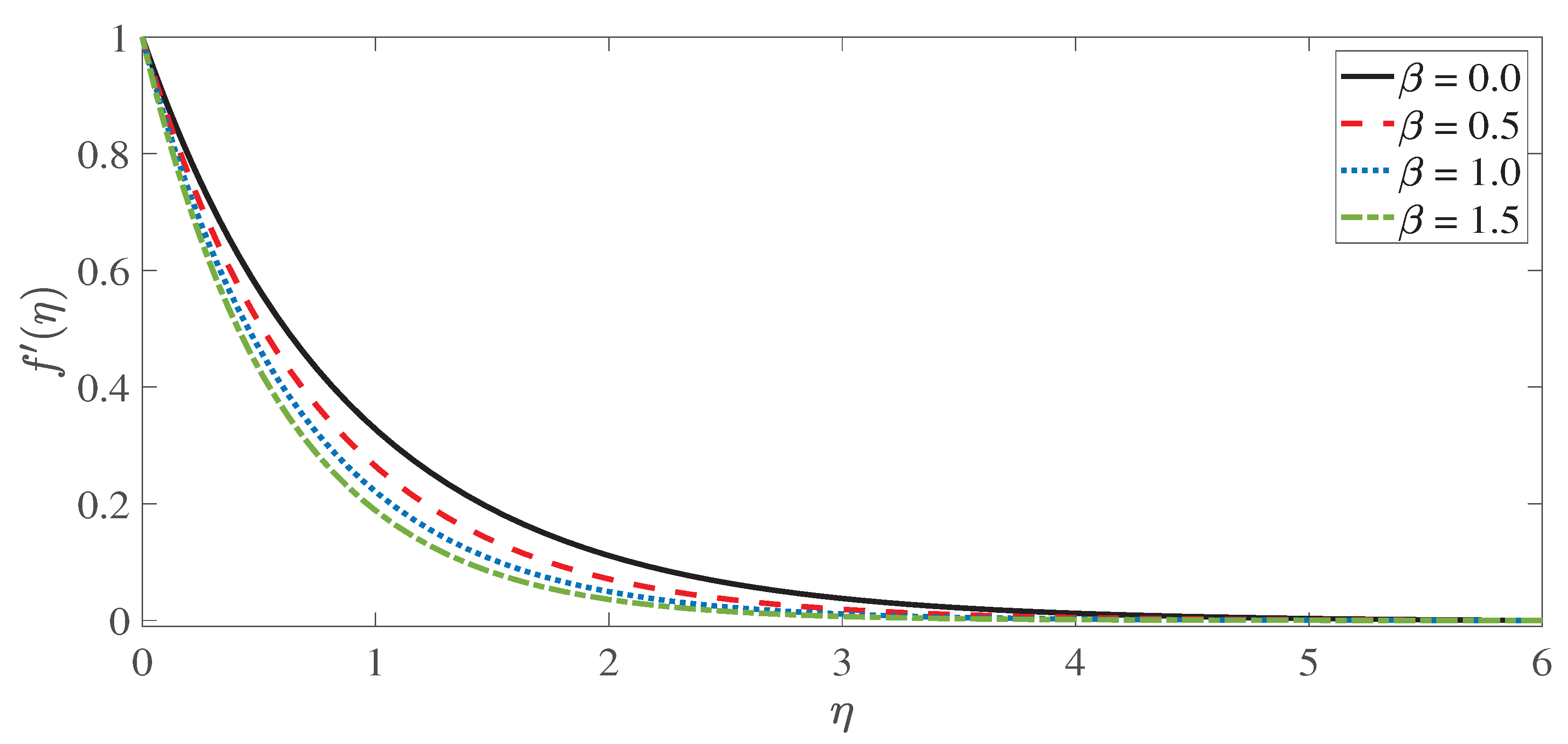
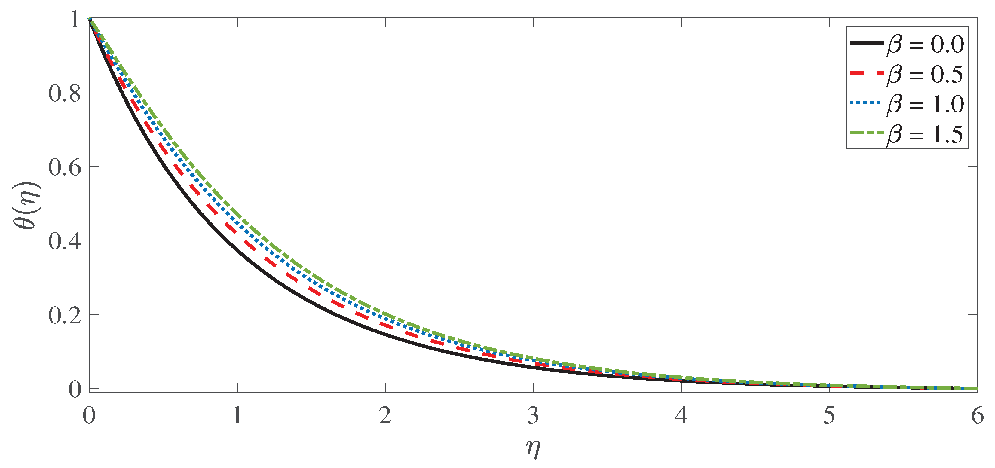
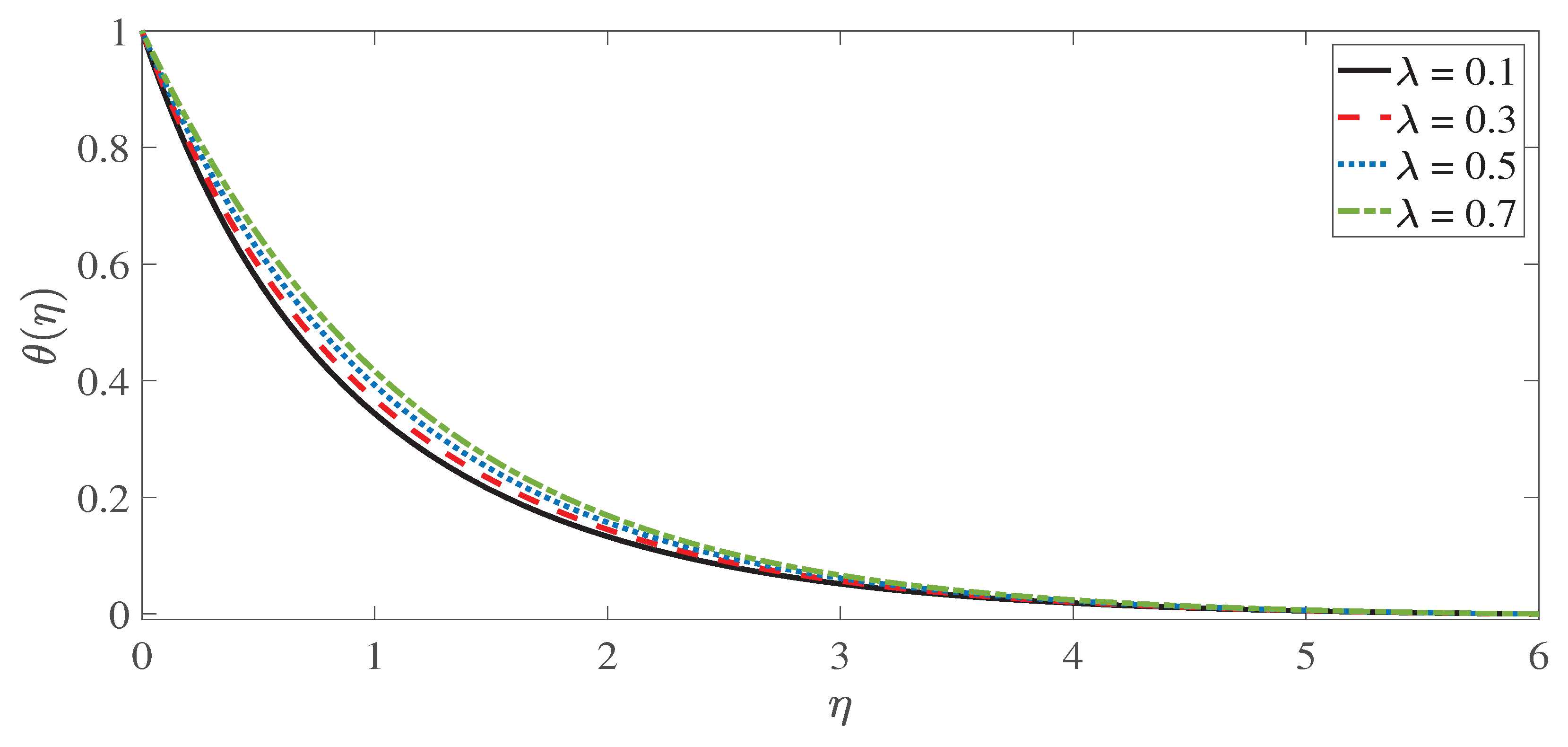
The magnetic and permeability parameters augment the temperature profile, while decreasing the velocity profile.
(ii)
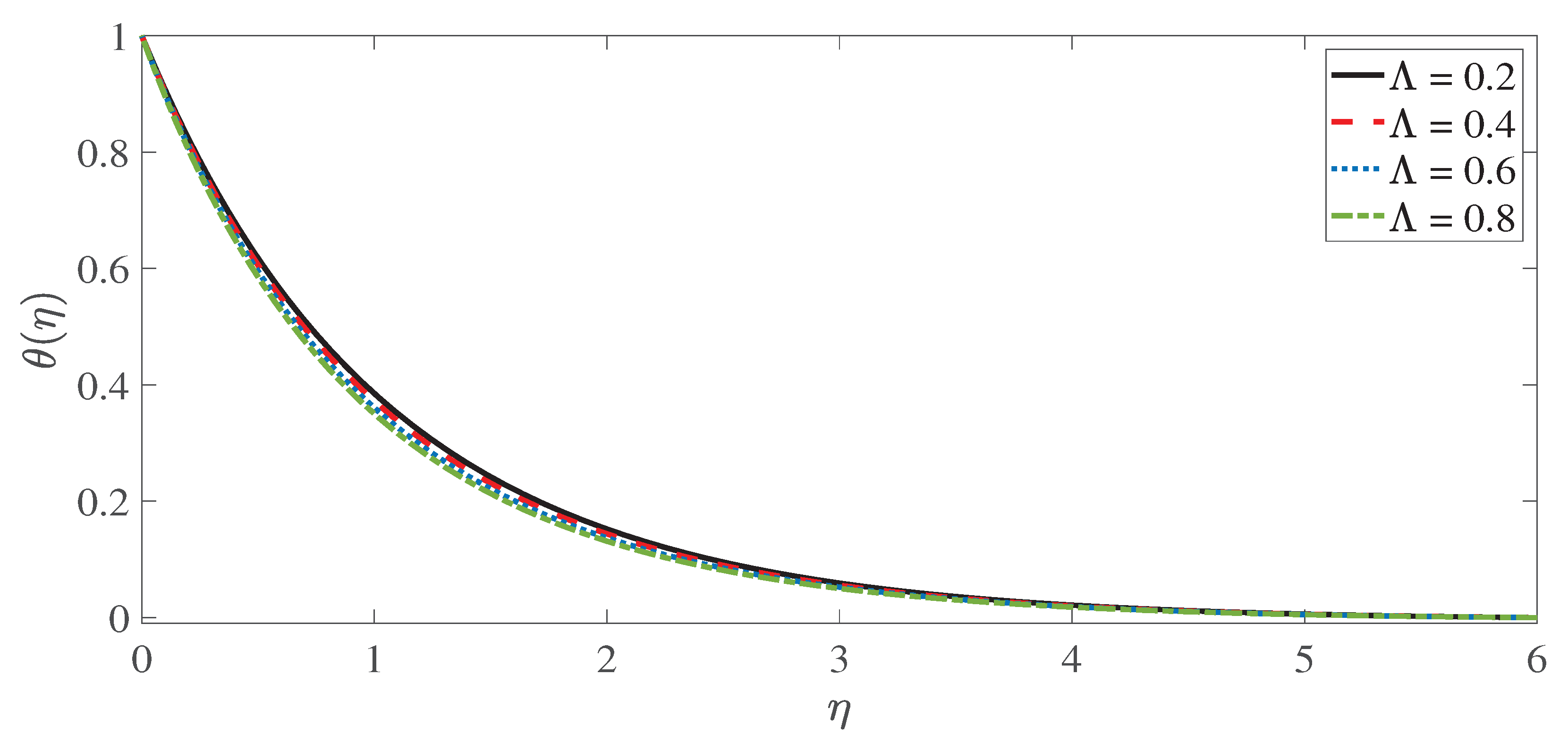
The mixed convection parameter increases the velocity profile, while reducing the temperature profile.
(iii)
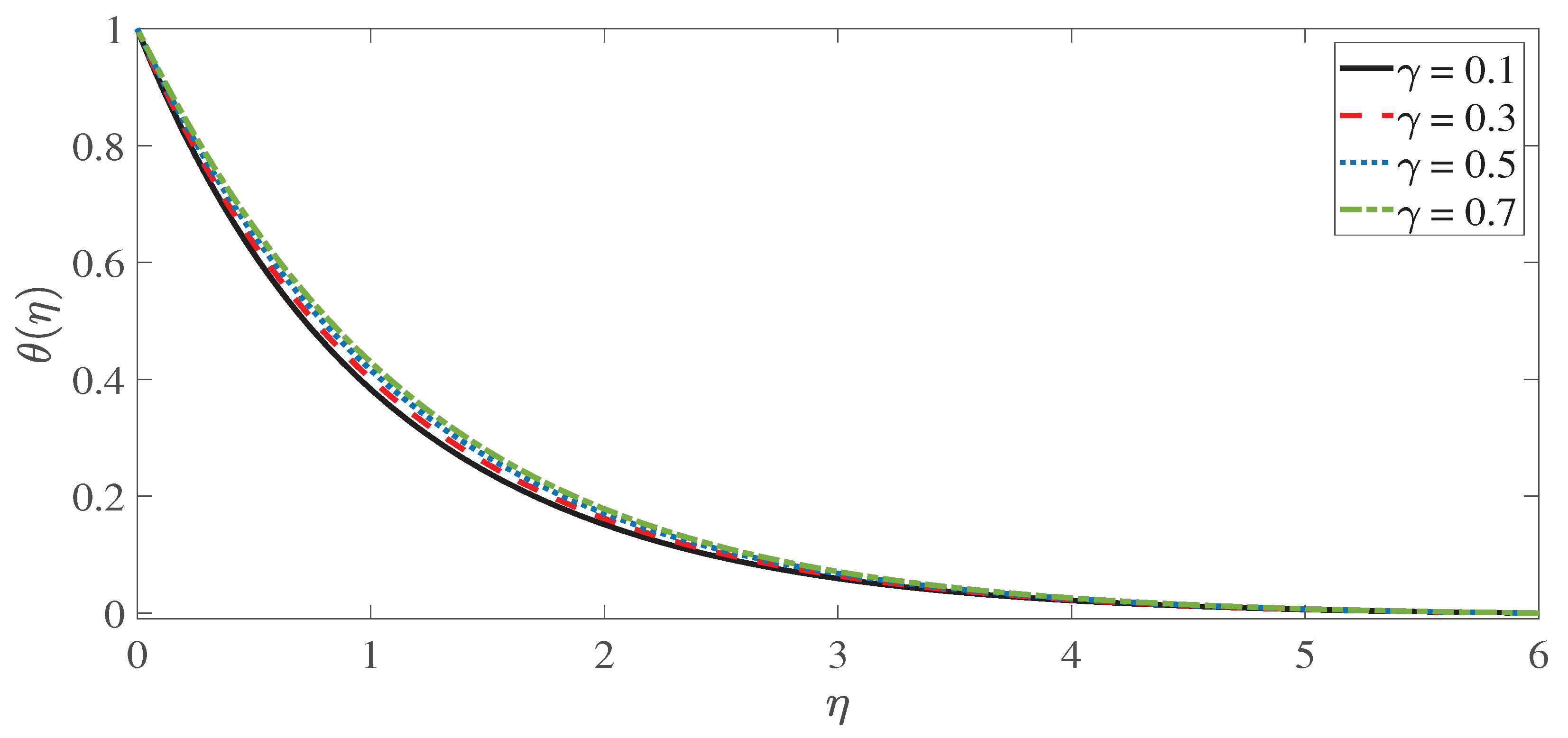
The Eckert number and the heat generation parameter have a significant effect to increase the temperature profile and the thickness of the thermal boundary layer.
(iv)
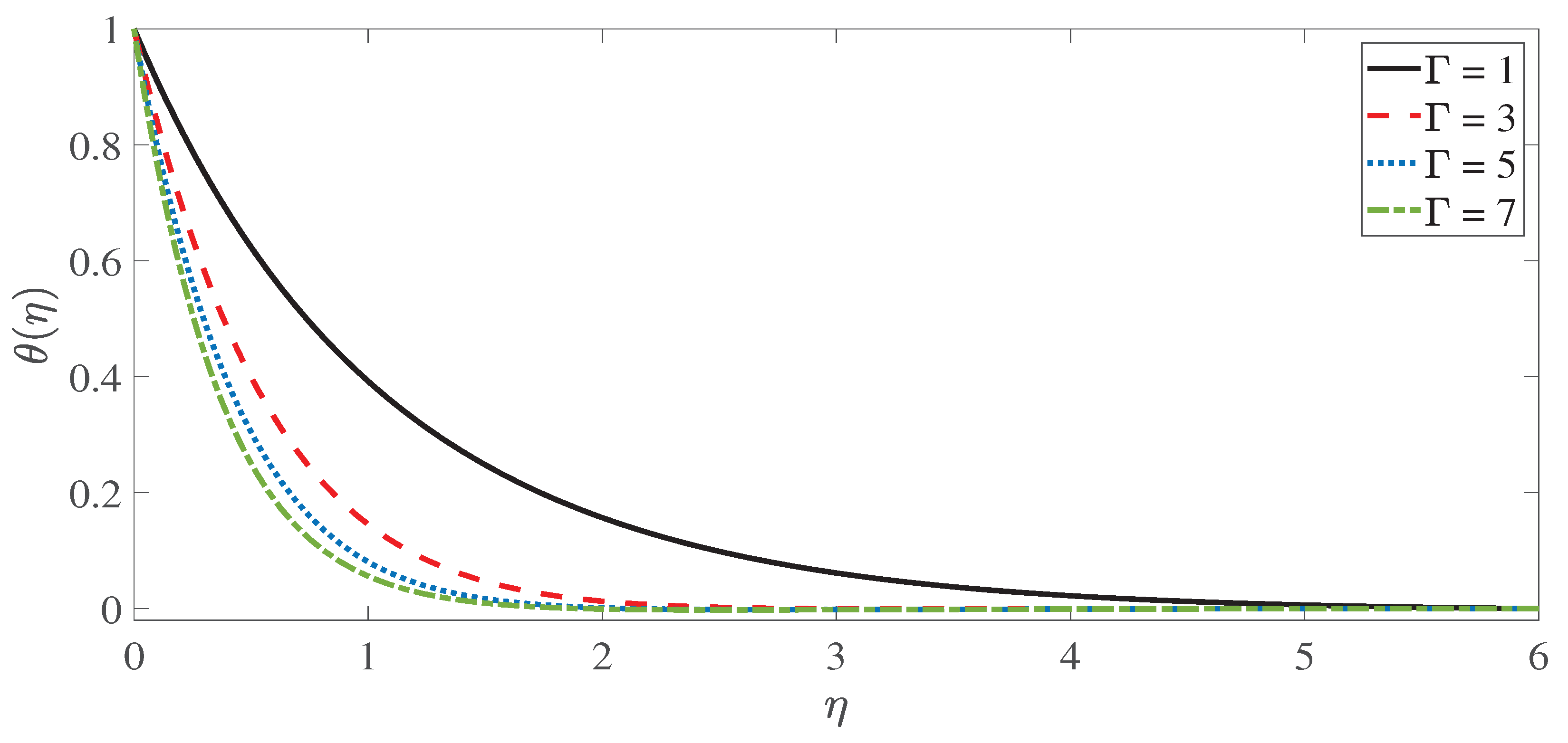
Increasing the Prandtl number reduces the temperature profile, because the momentum diffusivity is more dominant and the increased flow dampens the development of the temperature profile.
(v)
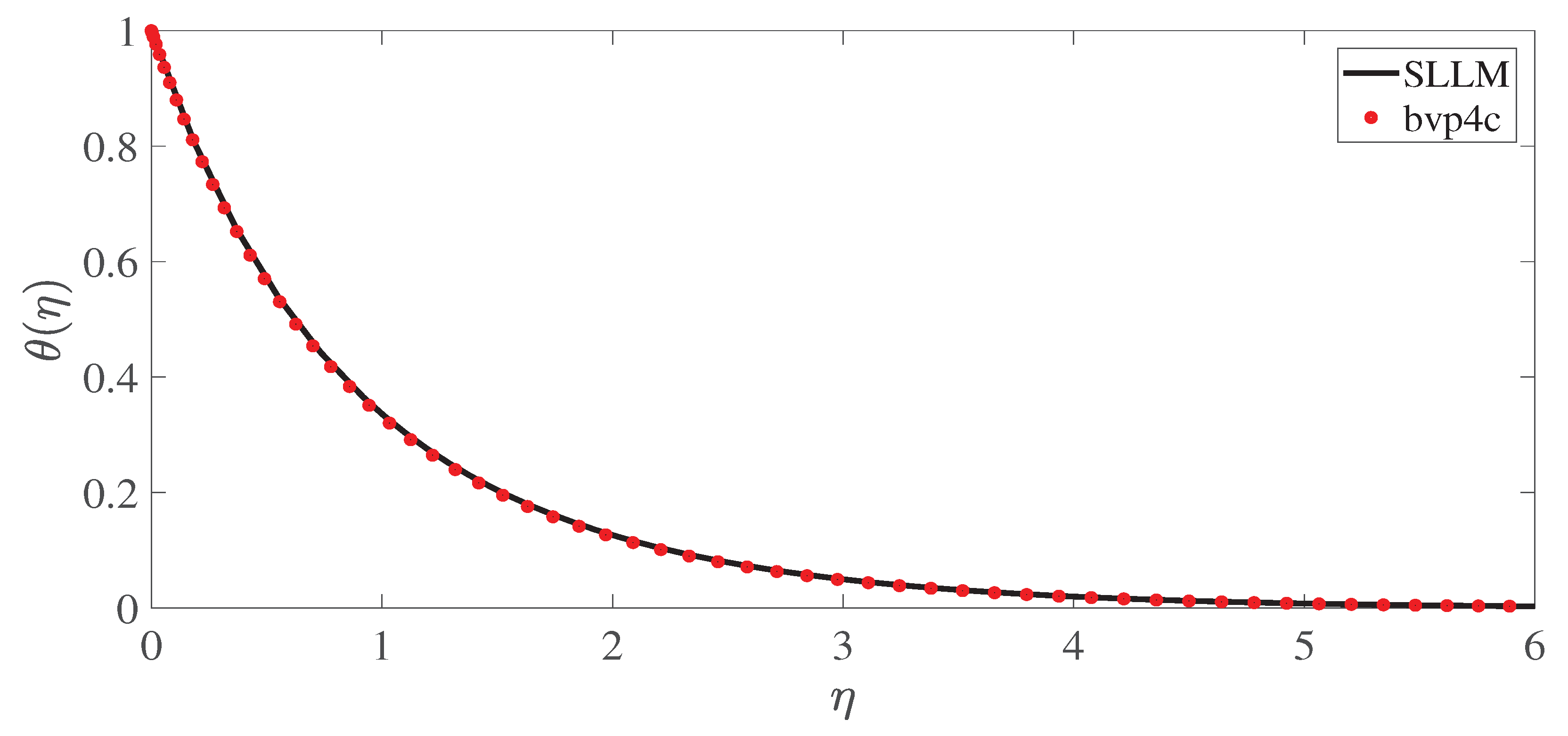
The numerical results obtained with the Spectral local linearization method are consistent with the results obtained with other related methodologies such as bvp4c.
(vi)
When the skin friction profile is compared to previously published data, it is found that the current numerical results show a good agreement and this validates the proposed method.
(vii)
The SLLM does not lose accuracy as the number of collocation points increases.
(viii)
For all of the model parameters investigated in this work, the method has been found to rapidly converge to the respective solutions.
(ix)
When compared to other approaches, the suggested methodology is computationally more efficient and shows better performance with fewer collocation points ( N ) and four iterations. Because this method is more reliable, simple, and efficient, the SLLM methodology is considered more suitable for the solution of nonlinear boundary value problems.
In general, the present analysis shows the excellent performance of the Spectral Local Linearization Method for the simulation of nonlinear boundary layer problems with porosity and viscous dissipation effects. Since our study is restricted to a Newtonian fluid model, future studies can be extended to non-Newtonian fluids with slip and no-slip effects.

Author Contributions

Conceptualization, L.Z. and M.M.B.; methodology, N.T.; software, N.T. and L.Z.; validation, M.M.B., L.Z. and E.E.M.; formal analysis, E.E.M. and L.Z.; investigation, N.T.; resources, L.Z. and M.M.B.; data curation, M.M.B.; writing—original draft preparation, N.T. and M.M.B.; writing—review and editing, L.Z. and E.E.M.; visualization, N.T. and L.Z.; supervision, L.Z. and M.M.B.; project administration, L.Z. and M.M.B.; funding acquisition, L.Z., N.T. and M.M.B. All authors have read and agreed to the published version of the manuscript.

Funding

This research was funded by National Natural Science Foundation of China No. 12172199.

Institutional Review Board Statement

Not applicable.

Informed Consent Statement

Not applicable.

Data Availability Statement

Not applicable.

Conflicts of Interest

The authors declare no conflict of interest.

References

  1. Janna, W.S. Engineering Heat Transfer; CRC Press: Boca Raton, FL, USA, 2018. [Google Scholar]
  2. Özisik, M.N.; Orlande, H.R. Inverse Heat Transfer: Fundamentals and Applications; CRC Press: Boca Raton, FL, USA, 2021. [Google Scholar]
  3. Kay, J.M.; Nedderman, R.M. An Introduction to Fluid Mechanics and Heat Transfer: With Applications in Chemical and Mechanical Process Engineering; Cambridge University Press: Cambridge, UK, 1975. [Google Scholar]
  4. McDonough, J. A perspective on the current and future roles of additive manufacturing in process engineering, with an emphasis on heat transfer. Therm. Sci. Eng. Prog. 2020, 19, 100594. [Google Scholar] [CrossRef]
  5. Rahmati, A.R.; Akbari, O.A.; Marzban, A.; Toghraie, D.; Karimi, R.; Pourfattah, F. Simultaneous investigations the effects of non-Newtonian nanofluid flow in different volume fractions of solid nanoparticles with slip and no-slip boundary conditions. Therm. Sci. Eng. Prog. 2018, 5, 263–277. [Google Scholar] [CrossRef]
  6. Sene, N. Second-grade fluid with Newtonian heating under Caputo fractional derivative: Analytical investigations via Laplace transforms. Math. Model. Numer. Simul. Appl. 2022, 2, 13–25. [Google Scholar] [CrossRef]
  7. Stangle, G.C.; Aksay, I.A. Simultaneous momentum, heat and mass transfer with chemical reaction in a disordered porous medium: Application to binder removal from a ceramic green body. Chem. Eng. Sci. 1990, 45, 1719–1731. [Google Scholar] [CrossRef] [Green Version]
  8. Polyanin, A.D.; Kutepov, A.M.; Kazenin, D.; Vyazmin, A. Hydrodynamics, Mass and Heat Transfer in Chemical Engineering; CRC Press: Boca Raton, FL, USA, 2001. [Google Scholar]
  9. Dogonchi, A.; Nayak, M.; Karimi, N.; Chamkha, A.J.; Ganji, D.D. Numerical simulation of hydrothermal features of Cu–H2O nanofluid natural convection within a porous annulus considering diverse configurations of heater. J. Therm. Anal. Calorim. 2020, 141, 2109–2125. [Google Scholar] [CrossRef]
  10. Cai, J.; Hajibeygi, H.; Yao, J.; Hassanizadeh, M. Advances in porous media science and engineering from InterPore2020 perspective. Adv.-Geo-Energy Res. 2020, 4, 352–355. [Google Scholar] [CrossRef]
  11. Nield, D.A.; Bejan, A. Convection in Porous Media; Springer: New York, NY, USA, 2006; Volume 3. [Google Scholar]
  12. Golparvar, A.; Zhou, Y.; Wu, K.; Ma, J.; Yu, Z. A comprehensive review of pore scale modeling methodologies for multiphase flow in porous media. Adv.-Geo-Energy Res. 2018, 2, 418–440. [Google Scholar] [CrossRef] [Green Version]
  13. Michaelides, E. Exergy Analysis for Energy Conversion Systems; Cambridge University Press: Cambridge, UK, 2021. [Google Scholar]
  14. Sakiadis, B.C. Boundary-layer behavior on continuous solid surfaces: I. Boundary-layer equations for two-dimensional and axisymmetric flow. AIChE J. 1961, 7, 26–28. [Google Scholar] [CrossRef]
  15. Crane, L.J. Flow past a stretching plate. Zeitschrift für angewandte Mathematik und Physik ZAMP 1970, 21, 645–647. [Google Scholar] [CrossRef]
  16. Roşca, A.V.; Pop, I. Flow and heat transfer over a vertical permeable stretching/shrinking sheet with a second order slip. Int. J. Heat Mass Transf. 2013, 60, 355–364. [Google Scholar] [CrossRef]
  17. Swain, I.; Mishra, S.; Pattanayak, H. Flow over exponentially stretching sheet through porous medium with heat source/sink. J. Eng. 2015, 2015, 452592. [Google Scholar] [CrossRef] [Green Version]
  18. Othman, N.A.; Yacob, N.A.; Bachok, N.; Ishak, A.; Pop, I. Mixed convection boundary-layer stagnation point flow past a vertical stretching/shrinking surface in a nanofluid. Appl. Therm. Eng. 2017, 115, 1412–1417. [Google Scholar] [CrossRef]
  19. Kumar, K.G.; Krishnamurthy, M.; Rudraswamy, N. Boundary layer flow and melting heat transfer of Prandtl fluid over a stretching surface by considering Joule heating effect. Multidiscip. Model. Mater. Struct. 2019, 15, 337–352. [Google Scholar] [CrossRef]
  20. Gangadhar, K.; Edukondala Nayak, R.; Venkata Subba Rao, M. Buoyancy effect on mixed convection boundary layer flow of Casson fluid over a non linear stretched sheet using the spectral relaxation method. Int. J. Ambient. Energy 2020, 1–9. [Google Scholar] [CrossRef]
  21. Prabha, G.S.S.; Bharathi, M.; Kudenatti, R.B. Heat transfer through mixed convection boundary layer in a porous medium: LTNE analysis. Appl. Therm. Eng. 2020, 179, 115705. [Google Scholar] [CrossRef]
  22. Badruddin, I.A.; Khan, T.Y.; Baig, M.A.A. Heat transfer in porous media: A mini review. Mater. Today Proc. 2020, 24, 1318–1321. [Google Scholar] [CrossRef]
  23. Ali, A.; Marwat, D.N.K.; Ali, A. Analysis of flow and heat transfer over stretching/shrinking and porous surfaces. J. Plast. Film Sheeting 2021, 38, 21–45. [Google Scholar] [CrossRef]
  24. Ilya, A.; Ashraf, M.; Ali, A.; Shah, Z.; Kumam, P.; Thounthong, P. Heat source and sink effects on periodic mixed convection flow along the electrically conducting cone inserted in porous medium. PLoS ONE 2021, 16, e0260845. [Google Scholar] [CrossRef]
  25. Adeniyan, A.; Mabood, F.; Okoya, S. Effect of heat radiating and generating second-grade mixed convection flow over a vertical slender cylinder with variable physical properties. Int. Commun. Heat Mass Transf. 2021, 121, 105110. [Google Scholar] [CrossRef]
  26. Winter, H. Viscous dissipation term in energy equations. Calc. Meas. Tech. Momentum Energy Mass Transf. 1987, 7, 27–34. [Google Scholar]
  27. Barletta, A.; Celli, M.; Rees, D.A. The onset of convection in a porous layer induced by viscous dissipation: A linear stability analysis. Int. J. Heat Mass Transf. 2009, 52, 337–344. [Google Scholar] [CrossRef]
  28. Jha, B.K.; Ajibade, A.O. Effect of viscous dissipation on natural convection flow between vertical parallel plates with time-periodic boundary conditions. Commun. Nonlinear Sci. Numer. Simul. 2012, 17, 1576–1587. [Google Scholar] [CrossRef]
  29. Ashraf, M.; Fatima, A.; Gorla, R. Periodic momentum and thermal boundary layer mixed convection flow around the surface of a sphere in the presence of viscous dissipation. Can. J. Phys. 2017, 95, 976–986. [Google Scholar] [CrossRef]
  30. Jafar, K.; Nazar, R.; Ishak, A.; Pop, I. MHD flow and heat transfer over stretching/shrinking sheets with external magnetic field, viscous dissipation and Joule effects. Can. J. Chem. Eng. 2012, 90, 1336–1346. [Google Scholar] [CrossRef]
  31. Dessie, H.; Kishan, N. MHD effects on heat transfer over stretching sheet embedded in porous medium with variable viscosity, viscous dissipation and heat source/sink. Ain Shams Eng. J. 2014, 5, 967–977. [Google Scholar] [CrossRef] [Green Version]
  32. Bibi, M.; Malik, M.; Tahir, M. Numerical study of unsteady Williamson fluid flow and heat transfer in the presence of MHD through a permeable stretching surface. Eur. Phys. J. Plus 2018, 133, 154. [Google Scholar] [CrossRef]
  33. Alarifi, I.M.; Abokhalil, A.G.; Osman, M.; Lund, L.A.; Ayed, M.B.; Belmabrouk, H.; Tlili, I. MHD flow and heat transfer over vertical stretching sheet with heat sink or source effect. Symmetry 2019, 11, 297. [Google Scholar] [CrossRef] [Green Version]
  34. Swain, B.; Parida, B.; Kar, S.; Senapati, N. Viscous dissipation and joule heating effect on MHD flow and heat transfer past a stretching sheet embedded in a porous medium. Heliyon 2020, 6, e05338. [Google Scholar] [CrossRef]
  35. Megahed, A.M.; Reddy, M.G.; Abbas, W. Modeling of MHD fluid flow over an unsteady stretching sheet with thermal radiation, variable fluid properties and heat flux. Math. Comput. Simul. 2021, 185, 583–593. [Google Scholar] [CrossRef]
  36. Sarada, K.; Gowda, R.J.P.; Sarris, I.E.; Kumar, R.N.; Prasannakumara, B.C. Effect of magnetohydrodynamics on heat transfer behaviour of a non-Newtonian fluid flow over a stretching sheet under local thermal non-equilibrium condition. Fluids 2021, 6, 264. [Google Scholar] [CrossRef]
  37. Zhou, J.C.; Abidi, A.; Shi, Q.H.; Khan, M.R.; Rehman, A.; Issakhov, A.; Galal, A.M. Unsteady radiative slip flow of MHD Casson fluid over a permeable stretched surface subject to a non-uniform heat source. Case Stud. Therm. Eng. 2021, 26, 101141. [Google Scholar] [CrossRef]
  38. Ullah, H.; Khan, I.; Fiza, M.; Hamadneh, N.N.; Fayz-Al-Asad, M.; Islam, S.; Khan, I.; Raja, M.A.Z.; Shoaib, M. MHD boundary layer flow over a stretching sheet: A new stochastic method. Math. Probl. Eng. 2021, 2021, 9924593. [Google Scholar] [CrossRef]
  39. Bhatti, M.M.; Jun, S.; Khalique, C.M.; Shahid, A.; Fasheng, L.; Mohamed, M.S. Lie group analysis and robust computational approach to examine mass transport process using Jeffrey fluid model. Appl. Math. Comput. 2022, 421, 126936. [Google Scholar] [CrossRef]
  40. Keskin, A.Ü. Solution of BVPs using bvp4c and bvp5c of MATLAB. In Boundary Value Problems for Engineers; Springer: Berlin/Heidelberg, Germany, 2019; pp. 417–510. [Google Scholar]
  41. Tabbakh, Z.; Ellaia, R.; Ouazar, D. Application of a local meshless modified characteristic method to incompressible fluid flows with heat transport problem. Eng. Anal. Bound. Elem. 2022, 134, 612–624. [Google Scholar] [CrossRef]
  42. Incropera, F.P.; Dewitt, D.P.; Bergman, T.L.; Lavine, A.S. Fundamentals of Heat and Mass Transfer; John Wiley & Sons Inc.: Hoboken, NJ, USA, 2002; 981p. [Google Scholar]
  43. Feng, Z.G.; Michaelides, E.E. Inclusion of heat transfer computations for particle laden flows. Phys. Fluids 2008, 20, 040604. [Google Scholar] [CrossRef]
  44. Shen, J.; Tang, T.; Wang, L.L. Spectral Methods: Algorithms, Analysis and Applications; Springer Science & Business Media: Berlin/Heidelberg, Germany, 2011; Volume 41. [Google Scholar]
  45. Fang, T.; Zhang, J.; Zhong, Y. Boundary layer flow over a stretching sheet with variable thickness. Appl. Math. Comput. 2012, 218, 7241–7252. [Google Scholar] [CrossRef]
  46. Prakash, D.; Muthtamilselvan, M.; Doh, D.H. Unsteady MHD non-Darcian flow over a vertical stretching plate embedded in a porous medium with non-uniform heat generation. Appl. Math. Comput. 2014, 236, 480–492. [Google Scholar]
Figure 1. Solution comparison of bvp4c and SLLM approach for velocity profile.
Fractalfract 06 00263 g001
Figure 2. Solution comparison of bvp4c and SLLM approach for temperature profile.
Fractalfract 06 00263 g002
Figure 3. Velocity profile for magnetic parameter β .
Fractalfract 06 00263 g003
Figure 4. Temperature profile for magnetic parameter β .
Fractalfract 06 00263 g004
Figure 5. Velocity profile for Permeability parameter γ .
Fractalfract 06 00263 g005
Figure 6. Temperature profile for permeability parameter γ .
Fractalfract 06 00263 g006
Figure 7. Temperature profile for local heat generation parameter δ .
Fractalfract 06 00263 g007
Figure 8. Temperature profile for Prandtl number Γ .
Fractalfract 06 00263 g008
Figure 9. Velocity profile for mixed convection parameter Λ .
Fractalfract 06 00263 g009
Figure 10. Temperature profile for mixed convection parameter Λ .
Fractalfract 06 00263 g010
Figure 11. Temperature profile as a function of Eckert number λ .
Fractalfract 06 00263 g011
Table 1. Applications of heat transfer through porous media.
Ceramic engineering [7]Simultaneous mass and heat transfer in disordered media occurs during the burnout/drying of the binder system from green compacts during the colloidal process of ceramics.
Chemical engineering [8]During the interim eventual and storage of nuclear waste, as well as in packet bed reactors.
Ground water hyrology [9]The investigation of seepage water through river beds and underground water resources.
Industrial engineering [10]The primary goal of filtration analysis is to examine the movement of fluid through a porous medium, leaving behind unwanted material. As a result of the mass deposition, the porous medium is constantly changing and altering the system’s pressure drop properties.
Mechanical engineering [11]To achieve effective insulation, solid conduction must be minimized, porosity must be maximized to reduce effective thermal conductivity, and free convection must be suppressed. The same concept is useful when producing high-performance insulators for cryogenic containers.
Petroleum engineering [12]For oil recovery mechanisms.
Geophysics [13]In the analysis of geo-pressurized reservoirs, and extraction of geothermal energy.
Table 2. Machine time to execute the Matlab code on intel core i7.
Function NameCallsTotal Time (s)Self Time (s)
SLLM code10.2840.202
Newplot20.0330.013
xlabel20.0290.023
newplot > ObserveAxesNextPlot20.0170.004
cla20.0130.007
hold20.0110.009
ylabel20.0100.008
convertStringToCharArgs40.0070.005
graphics/private/clo20.0050.005
gobjects40.0030.003
convertStringsToChars40.0020.001
markfigure20.0010.001
graphics/private/claNotify20.0010.001
graph2d/private/labelcheck40.0010.001
convertStringsToChars > convertStrings160.0010.001
axescheck20.0000.000
newplot > ObserveFigureNextPlo20.0000.000
Table 3. Impact of varying N on skin friction coefficient and Nusselt number.
IterationsNSkin Friction CoefficientNusselt Number
45 1.15627 1.17653
410 1.29290 1.43602
4100 1.30162 1.44072
bvp4c 1.30162 1.44072
Table 4. Numerical comparison between the present numerical method and bvp4c for Skin friction against different values of emerging parameters.
β γ Λ Γ δ λ ς ϕ SLLMbvp4c
0.20.20.510.10.201 1.30162 1.30162
1 1.65671 1.65671
1.5 1.85064 1.85064
0.5 1.44264 1.44264
0.8 1.57383 1.57383
1.2 1.73640 1.73640
0.4 1.34991 1.34991
1.0 1.07167 1.07167
1.5 0.85505 0.85505
0.71 1.27273 1.27273
2 1.40238 1.40238
3 1.44594 1.44594
0.1 1.31463 1.31463
0 1.30860 1.30860
0.12 1.30008 1.30008
0.3 1.29782 1.29782
0.4 1.29404 1.29404
0.5 1.29029 1.29029
0.5 1.00143 1.00143
0 1.301625 1.301625
0.5 1.70488 1.70488
0.6 0.942750 0.942750
0 0.45307 0.45307
0.6 0.48097 0.48097
Table 5. Numerical comparison between present method and bvp4c for Nusselt number against different values of the other parameters.
β γ Λ Γ δ λ SLLMbvp4c
0.20.20.510.10.2 1.44072 1.44072
1 1.25957 1.25957
1.5 1.16052 1.16052
0.5 1.36888 1.36888
0.8 1.30192 1.30192
1.2 1.21886 1.21886
0.4 1.42396 1.42396
1 1.50962 1.50962
1.5 1.56319 1.56319
0.71 1.18551 1.18551
2 2.15499 2.15499
3 2.69120 2.69120
0.1 1.55523 1.55523
0 1.49965 1.49965
0.12 1.42846 1.42846
0.3 1.38320 1.38320
0.4 1.32612 1.32612
0.5 1.26948 1.26948
Table 6. Numerical comparison between present results with previously report results [45] for skin friction profile.
β γ Λ ς ϕ Present ResultsFang et al. [45]
000 1 6 1 1.0234 1.0234
Publisher’s Note: MDPI stays neutral with regard to jurisdictional claims in published maps and institutional affiliations.

