
Parameter Estimation of LFM Signals Based on FOTD-CFRFT under Impulsive Noise
1
School of Information Engineering, Inner Mongolia University of Science and Technology, Baotou 014000, China
2
School of Science, Inner Mongolia University of Science and Technology, Baotou 014000, China
*
Author to whom correspondence should be addressed.
Fractal Fract. 2023, 7(11), 822; https://doi.org/10.3390/fractalfract7110822
Submission received: 13 September 2023
/
Revised: 27 October 2023
/
Accepted: 9 November 2023
/
Published: 15 November 2023
(This article belongs to the Special Issue Recent Advances in Fractional Fourier Transforms and Applications)
Abstract
:Due to the short duration and high amplitude characteristics of impulsive noise, these parameter estimation methods based on Gaussian assumptions are ineffective in the presence of impulsive noise. To address this issue, a LFM signal parameter estimation method is proposed based on FOTD and CFRFT. Firstly, the mathematical expression of FOTD is presented and its tracking performance is verified. Secondly, the tracked signal is subjected to discrete time CFRFT, and a mathematical optimization model for LFM signal parameter estimation is established on the fractional spectrum characteristic. Finally, a correction method for non-standard SαS distributed noise is proposed, and the performance of parameter estimation under both standard and non-standard SαS distributions are analyzed. The simulation results show that this method not only effectively suppresses the impact of impulsive noise on the fractional spectrum of LFM signal, but also has better parameter estimation accuracy and stability in the low GSNR. The proposed method is particularly effective under the measured noise environment, as it successfully suppresses the impact of impulsive noise and achieves high-precision parameter estimation.
1. Introduction
Linear frequency modulation (LFM) signal is a typical non-stationary signal, whose instantaneous frequency varies linearly with time. Compared with single frequency signal and narrow-band signal, LFM signal has stronger anti-interference ability; thus, it is widely used in radar, sonar, communication, seismic survey and other fields [1,2]. Due to the inevitable introduction of noise during signal acquisition and transmission, the parameter estimation of LFM signal under noisy environments is a common and fundamental issue in these fields. Most existing parameter estimation methods assume that the noise obeys a Gaussian distribution, but the noise caused by sudden interference in the actual environment generally does not obey the Gaussian distribution. Impulsive noise is a typical non-Gaussian noise, which has the characteristics of short duration and high amplitude. The performance of traditional methods degrades significantly under impulsive noise, and even cannot accurately estimate parameter. Therefore, it is necessary to explore the LFM signal parameter estimation method in the presence of impulsive noise.
To address the parameter estimation under impulsive noise environment, scholars have proposed many methods, such as, fractional lower-order statistics [3,4,5], nonlinear transform [6,7,8], tracking differentiator [9,10], convolutional neural networks [11,12]. In [3], an improved fractional lower order LVD (FLO-LVD) for the impulsive noise is proposed, which can overcome the influence of cross-terms and achieve higher estimation accuracy. In [5], FLO-SST with adaptive order and adaptive window is proposed, which utilizes FLO to suppress impulsive noise and obtain the instantaneous frequency of LFM signal by SST. However, these two methods require prior information of impulsive noise and lack theoretical support for selecting the order. In [7], the Sigmoid-FPSD method is proposed to effectively suppress impulsive noise, which has certain adaptability to changes in impulsive noise parameter. In [8], a piecewise nonlinear amplitude transformation (PNAT) function was designed to suppress impulsive noise, and combined with LVD to form a new LFM signal parameter estimation method, named PANT-LVD. However, these methods based on nonlinear transform also present certain drawbacks including poor stability under low GSNR and extensive computational requirements. In [9], fastest tracking differentiator (FTD) and fractional Fourier transform (FRFT) are proposed to estimate the parameter of LFM signal under impulsive noise. It effectively eliminates high-amplitude impulsive noise, but suffers a significant performance degradation under low GSNR and strong impulsive noise environments. In [12], a deep learning-based parameter estimation method of LFM signal is proposed, which uses deep neural networks and convolutional neural networks to eliminate the impact of impulsive noise on LFM signal parameter estimation. However, this method requires a considerable amount of time to train the model. It is necessary to point out that all these methods can only estimate parameter if the impulsive noise obeys a standard symmetric α-stable (SαS) distribution, the performance sharply decreases and even be unable to estimate parameter when impulsive noise does not obey the standard SαS distribution.
In recent years, with the development of fractional calculus theory, fractional calculus has expanded into the fields of science and engineering, particularly finding wide applications in control systems. Due to the limited performance of integer-order adaptive controllers, a fractional-order adaptive controller is designed to improve the performance and stability of the system by using a fractional-order tracking differentiator (FOTD). Therefore, research on FOTD is continuously being conducted in various fields. In [13], the design and analysis of FOTD are introduced, a fractional order self-disturbance rejection controller is designed by FOTD. In [14], the fractional order adaptive controller is designed by FOTD to obtain the differential signal, and the stability of the adaptive system is analyzed. In [15], a fractional order nonlinear disturbance observer based on FOTD is designed to improve the control performance of UAV in the disturbance environment.
Inspired by tracking differentiator, this paper presents a new application of FOTD in the LFM signal parameter estimation under impulsive noise environment. This method utilizes FOTD to track noisy signals and achieve a significant reduction of high-amplitude impulsive noise. Moreover, the fractional spectrum of the tracked signal is established by concise fractional Fourier transform (CFRFT), and a mathematical optimization model of parameter estimation is built on the fractional spectrum characteristic of LFM signal. Finally, a correction method for non-standard SαS distribution noise is proposed by using the properties of α-stable distribution, which effectively solves the LFM signal parameter estimation under non-standard SαS distribution noise. The main contributions of this paper include: (1) FOTD based on G-L fractional derivative is constructed and its discrete form is given; (2) FOTD is employed to suppress impulsive noise, and a FOTD-CFRFT based method is proposed to estimate LFM signal parameter in the presence of impulsive noise; (3) a correction method is proposed to effectively address the parameter estimation under non-standard SαS distribution noise.
The rest of this paper is arranged as follows: Section 2 briefly introduces the impulsive noise model, Section 3 proposes the LFM signal parameter estimation method, Section 4 conducts simulation experiments analysis and comparison for the simulated and measured impulsive noise, and Section 5 gives a brief summary.
2. Impulsive Noise Model
The impulsive noise typically exhibits characteristics of short duration and high amplitude, which can be fitted by the α-stable distribution model. The α-stable distribution does not have a closed-form probability density function, and is commonly represented by the following characteristic function [16,17]
with
where represents the sign function. denotes the characteristic exponent of impulsive noise, higher indicates weaker impulsive intensity. Similar to the variance in Gaussian distribution, denotes the dispersion coefficient, which reflects the deviation of samples from the mean. denotes the skewness parameter, describing the skewness of the distribution. represents the location parameter with the range of . When , the distribution is called as SαS distribution. When , the distribution is called as standard SαS distribution. Since the variance of α-stable distribution noise is undefined, GSNR is used to replace SNR, defined as
where represents the variance of the signal, and represents the dispersion coefficient of the impulsive noise.
Below, three common properties of α-stable distribution are briefly listed as [18]
- (1)
- If , is a real number, then
- (2)
- If , m is a non-zero real number, then
- (3)
- Let and be mutually independent α-stable distribution, thenwhere
3. Parameter Estimation Method
3.1. Fractional-Order Tracking Differentiator
The expression of FOTD can be obtained by using fractional-order optimal control theory and the design approach of integer-order tracker differentiator. The FOTD is defined as
where is the tracked signal, is the fractional derivative of , is the fastest control synthesis function. By passing the input signal to function, FOTD can quickly respond to the changes in input signal, and accurately compute its fractional derivative [19,20].
The fractional calculus used in this paper is the Grünwald–Letnikov definition, i.e.,
with
where denotes fractional derivative order, h denotes the differential step. The discrete form of FOTD is given by
with
where
is the discrete input signal, where , and is the sampling points number. and are the discrete forms of and . r denotes the tracking factor; the larger r is, the faster can track the signal . denotes the filtering factor; the smaller can give a better suppression on high-amplitude impulsive noise.
Figure 1a shows a pure LFM signal and its tracked signal ; it can be observed that has a certain phase delay and amplitude reduction. Compared with the original signal, amplitude reduction does not affect the parameter estimation, but the phase delay will directly affect the accuracy of parameter estimation. Therefore, the phase delay must be reduced as much as possible. Inspired by the displacement formula in physics, the tracked signal is corrected with the differential signal to approximate the original signal. The approximated signal is given by , where controls the approximation degree. From Figure 1b, the peak point locations show that has a smaller delay compared to , achieving the effect of reducing the phase delay.
3.2. Parameter Estimation Model
The expression of the LFM signal is
where is the amplitude, is the center frequency, and is the chirp rate. The definition of CFRFT for signal is [21]
where represents the rotation angle and represents the CFRFT of . The discrete-time CFRFT is given by
where . Further discretize the variable , the discrete CFRFT is given by
For CFRFT, the relationship between and can be expressed as
It means that the time axis is rotated by and stretched by , while the frequency axis is rotated by to obtain the new coordinate system (see Figure 2). LFM signal exhibits a linear change in frequency with respect to time in the time-frequency plane, where the slope of the line and its center are and , respectively. When the axis is orthogonal to the IF of LFM signal , the projection of the IF on axis is a point . Therefore, it can be concluded that when , the fractional spectrum of LFM signal is energy concentration.
In addition, according to Equations (15) and (16), the fractional spectrum of LFM signal is given by
Specifically, when , then
According to the Parseval’s theorem, i.e.,
It can be followed that the fractional spectrum of LFM signal reaches a global maximum at when .
Based on this characteristic, a mathematical model for LFM signal parameter estimation is established as
where represents the tracked signal. and denote the optimal value points, and represent the estimated chirp rate and center frequency, respectively. LFM signal exhibits energy concentration at a certain CFRFT domain, and the position of the peak is related to the parameter of LFM signal. Figure 3 shows the fractional spectrum of LFM signal in the CFRFT domain, a prominent peak can be observed. By performing peak search, the coordinates () of the peak can be substituted into Equation (23) to estimate the center frequency and chirp rate.
In this paper, the water cycle algorithm (WCA) is utilized to search for the global optimum. WCA is a metaheuristic algorithm inspired by the natural water cycle process, which combines the search for the optimum solution with the water cycle process in nature [22]. The algorithm flow of the proposed method is illustrated in Figure 4 and the specific steps are as follows:
Step 1: The pure LFM signal is generated by using Equation (15).
Step 2: A random impulsive noise is generated and added to , i.e., , where obeys the α-stable distribution, denotes the noisy signal.
Step 3: FOTD is applied to track the noisy signal, and the tracked signal is denoted as .
Step 4: The fractional spectrum of the tracked signal is established by using DTCFRFT, and LFM parameters are estimated by using Equation (23).
Step 5: 100 Monte Carlo experiments are performed, and an outlier detection algorithm is used to eliminate outliers.
4. Simulation Experiment
The simulation experiment is arranged as follows: The proposed FOTD-CFRFT method is initially analyzed, followed by a comparison with three other recently proposed methods under simulated impulsive noise. Lastly, the parameter estimation performance is tested in the presence of measured impulsive noise. The parameters of LFM signal in the simulation experiment are set by
where denotes sampling rate, T denotes sampling duration, N denotes the sampling number.
4.1. FOTD Analysis
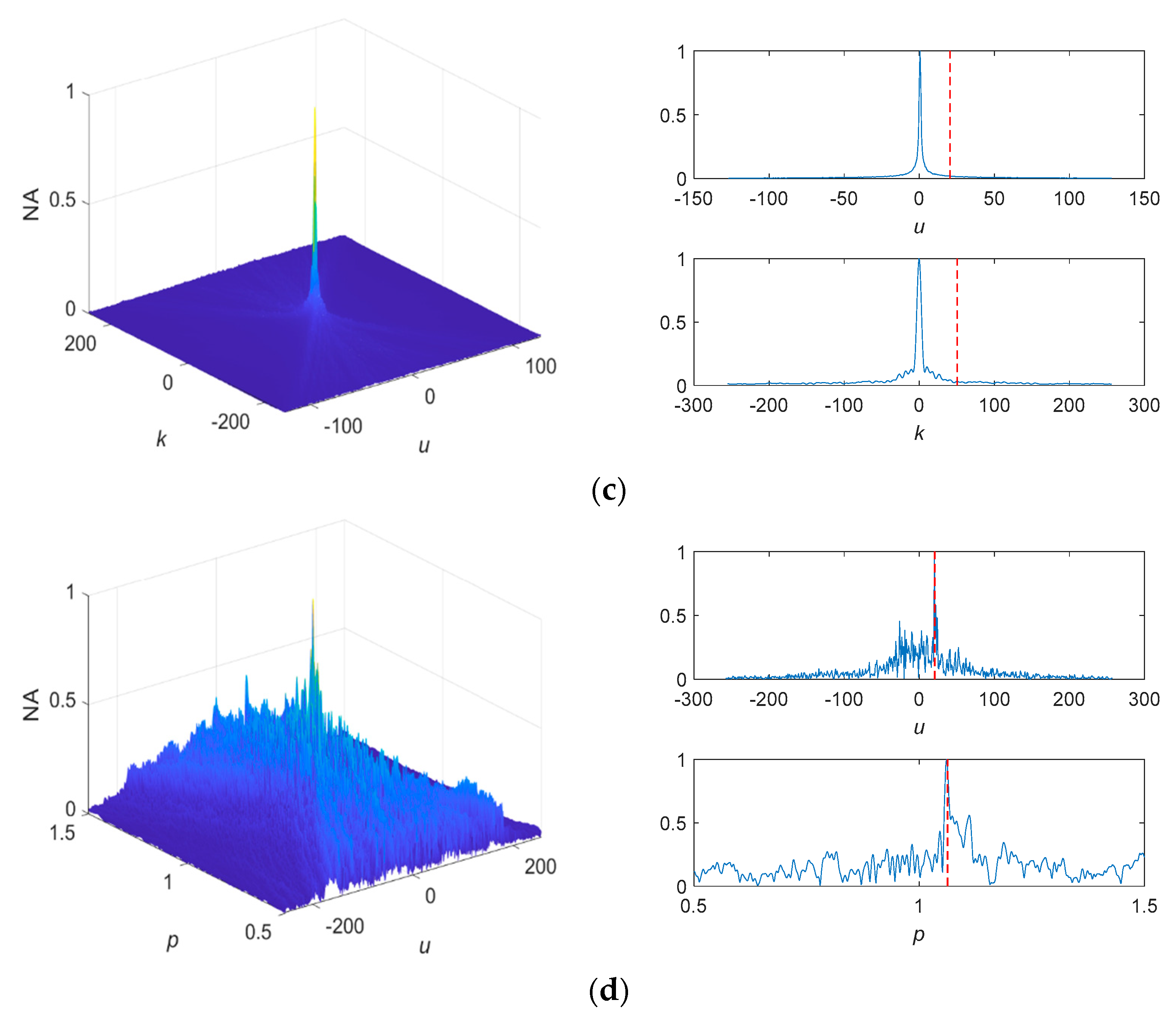
In this subsection, the tracking performance of FOTD is demonstrated, and the impact of each parameter on estimation accuracy is analyzed from an experimental perspective. Figure 5a shows the time-domain waveform of the noisy signal, which clearly shows the presence of numerous high-amplitude impulsive noises. Figure 5b shows the time-domain waveform of the tracked signal by FOTD. It can be observed that the high-amplitude impulsive noise has been suppressed, which provides favorable conditions for the accurate estimation of LFM signal parameter. Moreover, in order to clearly demonstrate the tracking effect of FOTD, the fractional spectrum of the noisy signal and tracked signal are shown in Figure 5c,d, respectively, where p denotes the rotational order, and NA denotes the normalized amplitude. It can be observed from Figure 5c that the true peak is obscured by the impulsive noise, resulting in inaccurate parameter estimation. However, the clear peak can be seen in Figure 5d, and the positions of the peak closely match the true values .
Since FOTD contains three parameters , it is necessary to analyze the impact of each parameter on the parameter estimation accuracy. By selecting different parameters, 100 Monte Carlo experiments were conducted under a standard SαS noise environment with . The RMSE of estimated results corresponding to each parameter are shown in Figure 6. From Figure 6, it can be seen that r has almost no impact on the parameter estimation, whereas the other two parameters directly affect the accuracy of parameter estimation. For the superior performance of FOTD, should be within the range of , and should be within the range of . Therefore, the parameters of FOTD are set as in the following sections.
4.2. Comparisons
4.2.1. Standard SαS Distribution Noise
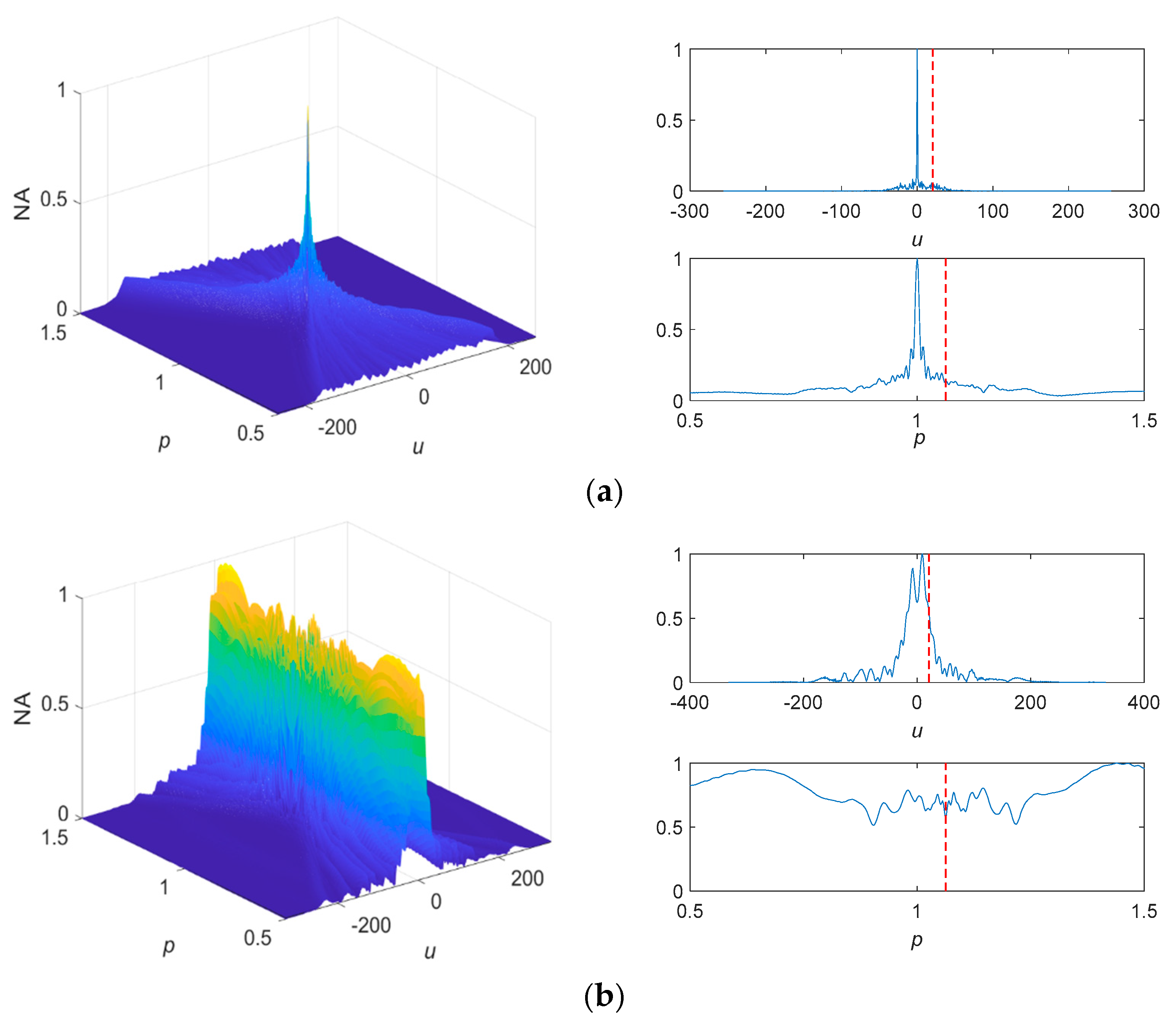
In order to better demonstrate the performance of parameter estimation under the impulsive noise, the proposed method is compared with the three newly proposed parameter estimation methods, i.e., Sigmoid-FPSD [7], PANT-LVD [8] and FTD-FRFT [9]. For and , the fractional spectrums of the noisy signal are built and shown in Figure 7, the search step size for parameter p is 0.002. From Figure 7, all four methods can suppress the impulsive noise and achieve accurate parameter estimation. However, the FTD-FRFT method shows significant noise amplitude in the fractional spectrum, which indicates poor suppression performance for impulsive noise.
To further compare the performance of four methods under low GSNR, the fractional spectrum of the noisy signal and its projection are constructed at , where the red lines represent the accurate positions of peak point. When , it can be observed from Figure 8 that the FTD-FRFT method fails to suppress the impulsive noise, and the peaks are submerged by the impulsive noise, resulting in inaccurate parameter estimation. However, Sigmoid-FPSD, PANT-LVD and FOTD-CFRFT methods can suppress the impulsive noise and achieve accurate parameter estimation.
Next, 100 Monte Carlo experiments are conducted at each GSNR level to calculate RMSE with , the average values of estimation results at different GSNR are presented in Table 1. It is evident from Table 1 that the FOTD-CFRFT method exhibits superior accuracy at high GSNR compared to the other three methods, whereas it remains effective when the other three methods fail to accurately estimate the parameters at low GSNR. To visually compare the performance of four methods at different GSNR levels, the RMSE of the estimated parameters for four methods are shown in Figure 9. From Figure 9a,b, it can be seen that the FTD-FRFT method can accurately estimate the LFM signal parameter when , whereas other three methods can accurately estimate the LFM signal parameter when . The FOTD-CFRFT method has a much smaller RMSE over the other three methods, which indicates that the FOTD-CFRFT method has stronger noise robustness. However, when GSNR decreases to , the estimation accurate of the FOTD-CFRFT method also drops sharply. The estimated parameters of 100 Monte Carlo experiments are shown as a scatter diagram in Figure 10, where the blue line represents the true IF of LFM signal. It can be observed that the FOTD-CFRFT method only has a small number of outliers occur in 100 Monte Carlo experiments, which means that the FOTD-CFRFT method has higher stability compared with the other three methods at low GSNR. Therefore, an outlier detection algorithm is applied to detect and remove these outliers for improving accuracy. Figure 9c,d show that the FOTD-CFRFT method combined with the outlier detection algorithm can effectively improve the accuracy of parameter estimation under low GSNR.
The influence of parameter on the parameter estimation accuracy is discussed above, then the parameter is analyzed below, where is varied in [0.2, 2] at . From Figure 11, it can be seen that the FTD-FRFT method can only estimate the parameter in a weak impulsive noise environment; its performance sharply declines under a strong impulsive noise environment. Different from FTD-FRFT, the other three methods can estimate the parameter under a strong impulsive noise environment, and RMSE is basically unaffected by the impulsive intensity. In summary, the proposed FOTD-CFRFT method is superior to Sigmoid-FPSD, PANT-LVD and FTD-FRFT methods in terms of noise robustness and stability.
4.2.2. Non-Standard SαS Distribution Noise
When the parameters or , the noise no longer obeys a standard SαS distribution, it is necessary to explore the parameter estimation performance under non-standard SαS distribution noise. Based on the properties of α-stable distribution listed in Equations (4)–(7), the non-standard SαS distribution can be corrected to a standard SαS distribution if α-stable distribution parameters are known. Therefore, the α-stable distribution noise parameters need to be estimated first. Assume the noise obeys α-stable distribution, denoted as , the specific correction methods are given by:
- (1)
- When , the correction formula is
- (2)
- When , let , the correction formula is
- (3)
- When , let , the correction formula is
The other parameters of noise are fixed as , the symmetric parameter is varied in . With different , the RMSE of center frequency and chirp rate for four methods are shown in Figure 12. It can be seen that the FTD-FRFT method can accurately estimate the parameter for , the Sigmoid-FPSD method can accurately estimate the parameter when , the PANT-LVD method can accurately estimate the parameter when . The Sigmoid-FPSD and PANT-LVD methods have some adaptability to , but they fail to accurately estimate the parameter when changes significantly. Figure 12 indicated that the FOTD-CFRFT method combined with the correction method can effectively solve the parameter estimation under the non-standard SαS distribution noise. To visually demonstrate the impact of , Figure 13 shows the fractional spectrum of tracked signal when . It can be seen that the FTD-FRFT, Sigmoid-FPSD and PANT-LVD methods cannot extract the fractional spectrum characteristic of LFM signal, and thus cannot accurately estimate the parameter. However, the proposed method combining FOTD-CFRFT and noise correction can accurately estimate the parameters of the LFM signal, indicating the effectiveness of the correction method.
In addition, the other parameters of noise are fixed as , Figure 14 shows the RMSE of parameter estimation when the parameter varies in . From Figure 14, the FTD-FRFT and PANT-LVD methods can accurately estimate the parameter only if . The Sigmoid-FRFT method can estimate the parameter when , which shows some adaptability to the variation in . However, with the increase in , the Sigmoid-FRFT method does not give an accurate estimation value. Combined with the noise correction method, the proposed FOTD-CFRFT achieves accurate parameter estimation for . With , the fractional spectrums of the tracked signal are shown in Figure 15. When , the noise is no longer a standard SαS distribution noise; therefore, the other three methods fail to extract the fractional spectrum characteristic of the LFM signal. Due to the combination of noise correction, the FOTD-CFRFT method can still accurately extract the fractional spectrum characteristic of LFM signal, so as to achieve high precision parameter estimation under the non-standard SαS distribution noise.
4.3. Measured Noise Experiment
To verify the effectiveness of the proposed method in a natural noisy environment, a measured impulsive noise was obtained from killer whale echolocation clicks recorded in the Glacier Bay National Preserve (see Figure 16) [23]. A segment of the noise was extracted and added to the LFM signal. GSNR is varied by adjusting the noise amplitude.
To analyze the performance of four methods under weak impulsive noise, a segment of noise was extracted from the 352,000th point to the 352,512th point, and further added to LFM signal. At this time, the GSNR is approximately . Since most measured noises do not typically obey a standard SαS distribution, correction is required before parameter estimation. The noise parameters are estimated by using noisy signal, and the obtained parameters are . Then, the noisy signal is corrected using Equation (27). Based on four methods, Figure 17 shows the fractional spectrum of LFM signal and its projections under the weak measured impulsive noise. From Figure 17, it can be observed that the FTD-FRFT and PANT-LVD methods fail to accurately estimate the parameter, while the Sigmoid-FPSD and FOTD-CFRFT methods can accurately estimate parameter. In terms of accuracy, the estimated center frequency and chirp rate by the Sigmoid-FPSD method are 21.10 Hz and 50.02 Hz/s. The corresponding results obtained by the FOTD-CFRFT method are 20.33 Hz and 50.12 Hz/s, which have better accuracy than that of Sigmoid-FPSD.
To compare the performance of four methods under a strong measured impulsive noise environment, a segment of 1,125,000 points to 1,125,512th point is extracted and added to LFM signal. As shown in Figure 18, the FTD-FRFT, Sigmoid-FPSD and PANT-LVD methods are unable to accurately estimate the parameters. Similar to weak impulsive noise case, the estimated noise parameters are . The proposed FOTD-CFRFT combined with noise correction can accurately estimate the parameter, the estimated center frequency and chirp rate are 20.39 Hz and 49.94 Hz/s, respectively. In summary, compared with the other three methods, the FOTD-CFRFT method combined with the noise correction method also has a much better performance under the measured impulsive noise environment.
5. Conclusions
In this paper, a fractional-order tracking differentiator (FOTD) based on G-L fractional derivative and its discrete form is constructed. Additionally, FOTD is utilized to suppress large impulsive noise, and an LFM signal parameter estimation method under impulsive noise is proposed using FOTD-CFRFT, which effectively addresses the issue that traditional parameter estimation methods perform poorly in the presence of impulsive noise. The experimental results show that the proposed method can effectively suppress high impulsive noise through FOTD, and overcome the disadvantage that the performance of the similar FTD-FRFT method sharply decreases under strong impulsive noise and low GSNR environment. In addition, the proposed method exhibits higher stability and accuracy than the Sigmoid-FPSD and PANT-LVD methods under low GSNR. Finally, since most actual environmental impulsive noise typically obeys a non-standard SαS distribution, a correction method for non-standard SαS distribution noises is proposed, which successfully achieves accurate estimation of LFM signal parameters under measured impulsive noise.
Author Contributions
Conceptualization, H.W. and Y.G.; methodology, H.W. and Y.G.; validation, H.W. and Y.G.; formal analysis, Y.G. and L.Y.; investigation, Y.G. and L.Y.; writing—original draft preparation, H.W., Y.G. and L.Y.; writing—review and editing, H.W., Y.G. and L.Y.; funding acquisition, Y.G. All authors have read and agreed to the published version of the manuscript.
Funding
This research was funded by the National Natural Science Foundation of China, no. 62161040, 62201298, 12261067.
Institutional Review Board Statement
Not applicable.
Informed Consent Statement
Not applicable.
Data Availability Statement
Data underlying the results presented in the paper are not publicly available at this time but may be obtained from the authors upon reasonable request.
Conflicts of Interest
The authors declare no conflict of interest.
References
- Bai, G.; Cheng, Y.; Tang, W.; Li, S. Chirp Rate Estimation for LFM Signal by Multiple DPT and Weighted Combination. IEEE Signal Process. Lett. 2019, 26, 149–153. [Google Scholar] [CrossRef]
- Li, T.; Hu, R.; Zhang, Z.; Wang, H. A time delay estimation method of LFM hybrid signals based on hough transform. In Proceedings of the 2021 IEEE 5th Advanced Information Technology, Electronic and Automation Control Conference, Chongqing, China, 12–14 March 2021; pp. 1457–1460. [Google Scholar]
- Jin, Y.; Duan, P.; Ji, H. Estimation of LFM signal parameters based on LVD in complex noise environment. J. Electron. Inf. Technol. 2014, 36, 1106–1112. [Google Scholar]
- Wang, H.; Long, J. Applications of fractional lower order synchrosqueezing transform time frequency technology to machine fault diagnosis. Math. Probl. Eng. 2020, 2020, 3983242. [Google Scholar] [CrossRef]
- Li, L.; Yu, X.; Jiang, Q.; Zang, B.; Jiang, L. Synchrosqueezing transform meets α-stable distribution: An adaptive fractional lower-order SST for instantaneous frequency estimation and non-stationary signal recovery. Signal Process. 2022, 201, 108683. [Google Scholar] [CrossRef]
- Chen, M.; Xing, H.; Wang, H. Multipath delay estimation of LFM signals based on NAT function under impulse noise. J. Electron. Meas. Instrum. 2022, 36, 73–81. [Google Scholar]
- Li, L.; Qiu, T. A robust parameter estimation of LFM signal based on sigmoid transform under the alpha stable distribution noise. Circuits Syst. Signal Process. 2019, 38, 3170–3186. [Google Scholar] [CrossRef]
- Wang, H.; Zhang, Q.; Cheng, W.; Dong, J.; Liu, X. A novel parameter estimation method based on piecewise nonlinear amplitude transform for the LFM signal in impulsive noise. Electronics 2023, 12, 2530. [Google Scholar] [CrossRef]
- Liu, X.; Li, X.; Xiao, B.; Wang, C.; Ma, B. LFM signal parameter estimation via FTD-FRFT in impulse noise. Fractal Fract. 2023, 7, 69. [Google Scholar] [CrossRef]
- Xiao, B.; Liu, X.; Wang, C.; Wang, Y.; Huang, T. Sliding-Window TD-FrFT algorithm for high-precision ranging of LFM signals in the presence of impulse noise. Fractal Fract. 2023, 7, 679. [Google Scholar] [CrossRef]
- Lu, J.; Guo, Y.; Yang, L. Denoising method for LFM signals based on DCNN under pulse noise. Mod. Radar 2023, 7, 1–11. [Google Scholar]
- Razzaq, H.S.; Hussain, Z.M. Instantaneous frequency estimation of FM signals under Gaussian and symmetric α-stable noise: Deep learning versus time–frequency analysis. Information 2022, 14, 18. [Google Scholar] [CrossRef]
- Wei, J.; Gao, Z. Design and analysis on fractional-order tracking differentiator. In Proceedings of the 27th Chinese Control and Decision Conference, Qingdao, China, 23–25 May 2015; pp. 3137–3141. [Google Scholar]
- Wei, Y.; Hu, Y.; Song, L.; Wang, Y. Tracking differentiator based fractional order model reference adaptive control: The 1<α<2 Case. In Proceedings of the 53rd IEEE Conference on Decision and Control, Los Angeles, CA, USA, 15–17 December 2014; pp. 6902–6907. [Google Scholar]
- Park, S.; Han, S. Robust backstepping control combined with fractional-order tracking differentiator and fractional-order nonlinear disturbance observer for unknown quadrotor UAV systems. Appl. Sci. 2022, 12, 11637. [Google Scholar] [CrossRef]
- Huang, X.; Zhang, L.; Chen, Z.; Zhao, R. Robust detection and motion parameter estimation for weak maneuvering target in the alpha-stable noise environment. Digit. Signal Process. 2021, 108, 102885. [Google Scholar] [CrossRef]
- Liu, X.; Wang, C. A novel parameter estimation of chirp signal in α-stable noise. IEICE Electron. Express 2017, 14, 20161053. [Google Scholar] [CrossRef]
- Liu, T. Research on Cyclic Stationary Signal Processing Method under Alpha Stable Distributed Noise; Dalian University of Technology: Dalian, China, 2020. [Google Scholar]
- Wei, Y.; Du, B.; Cheng, S.; Wang, Y. Fractional Order Systems Time-Optimal Control and Its Application. J. Optim. Theory Appl. 2017, 174, 122–138. [Google Scholar] [CrossRef]
- Sun, B.; Sun, X. Composite function for optimal control of discrete systems. Control. Decis. 2010, 25, 473–477. [Google Scholar]
- Guo, Y.; Yang, L. Method for parameter estimation of LFM signal and its application. IET Signal Process. 2019, 13, 538–543. [Google Scholar] [CrossRef]
- Eskandar, H.; Sadollah, A.; Bahreininejad, A.; Hamdi, M. Water cycle algorithm—A novel metaheuristic optimization method for solving constrained engineering optimization problems. Comput. Struct. 2012, 110–111, 151–166. [Google Scholar] [CrossRef]
- Sounds Recorded in Glacier Bay. Available online: https://www.nps.gov/glba/learn/nature/soundclips.htm (accessed on 10 July 2023).
Figure 1.
The tracked signal of FOTD and improved FOTD: (a) FOTD; (b) improved FOTD.
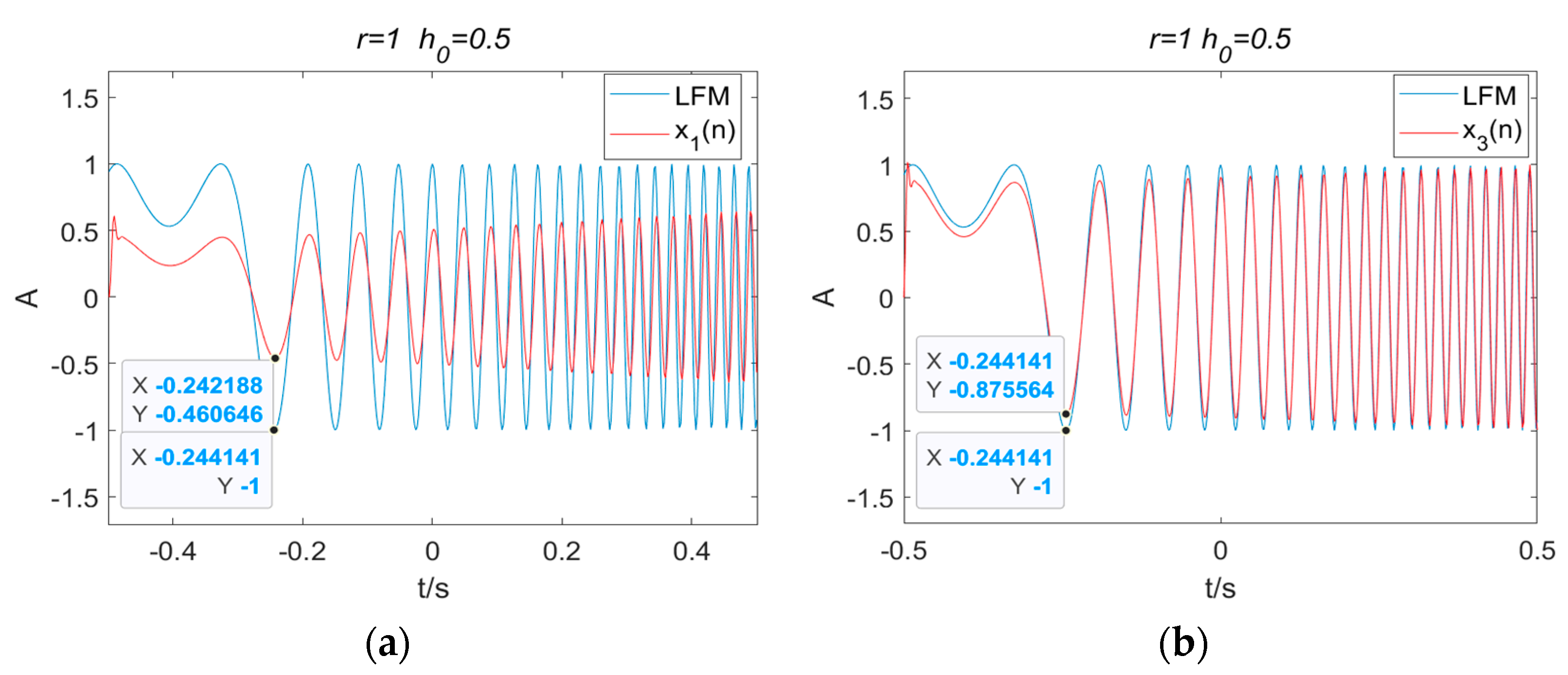
Figure 2.
The principle of CFRFT for LFM signal.

Figure 3.
The fractional spectrum of LFM signal established by CFRFT.
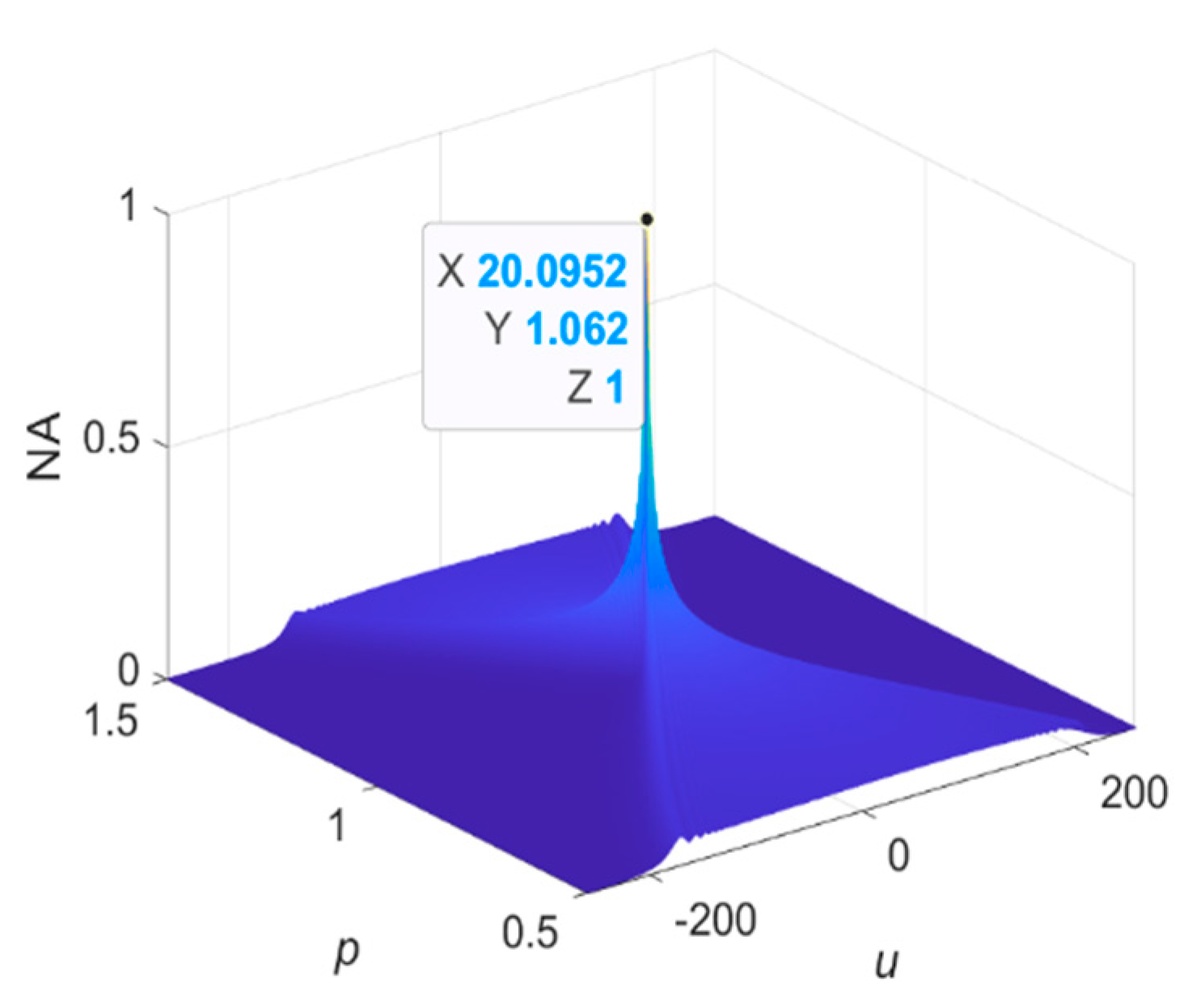
Figure 4.
Flow chart of FOTD-CFRFT algorithm.

Figure 5.
The tracking performance of FOTD: (a) time-domain waveform of the noisy signal; (b) time-domain waveform of the tracked signal; (c) fractional spectrum of the noisy signal; (d) fractional spectrum of the tracked signal.
Figure 5.
The tracking performance of FOTD: (a) time-domain waveform of the noisy signal; (b) time-domain waveform of the tracked signal; (c) fractional spectrum of the noisy signal; (d) fractional spectrum of the tracked signal.
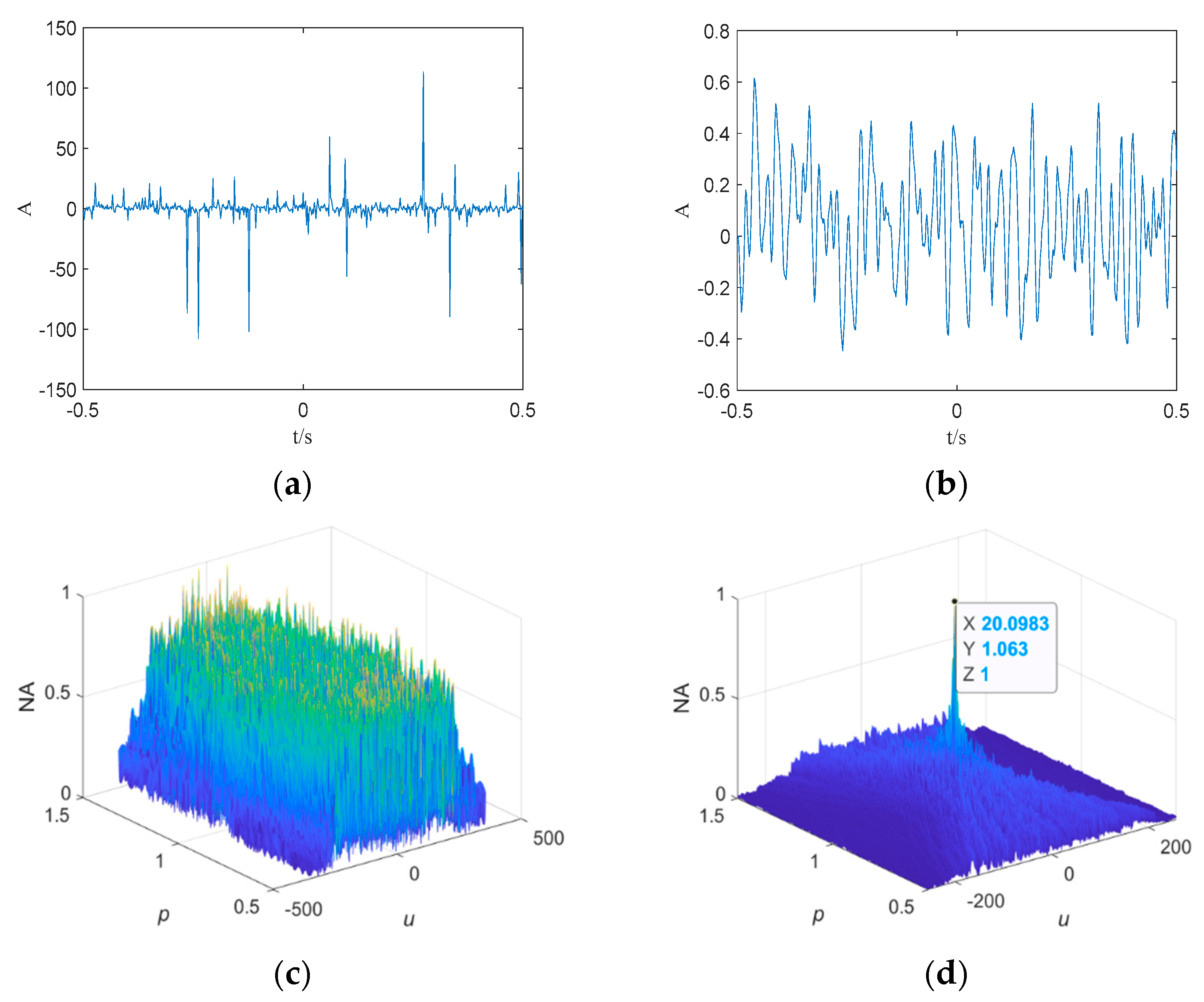
Figure 6.
The parameter analysis of FOTD: (a) tracking factor r; (b) filtering factor ; (c) fractional derivative order .
Figure 6.
The parameter analysis of FOTD: (a) tracking factor r; (b) filtering factor ; (c) fractional derivative order .
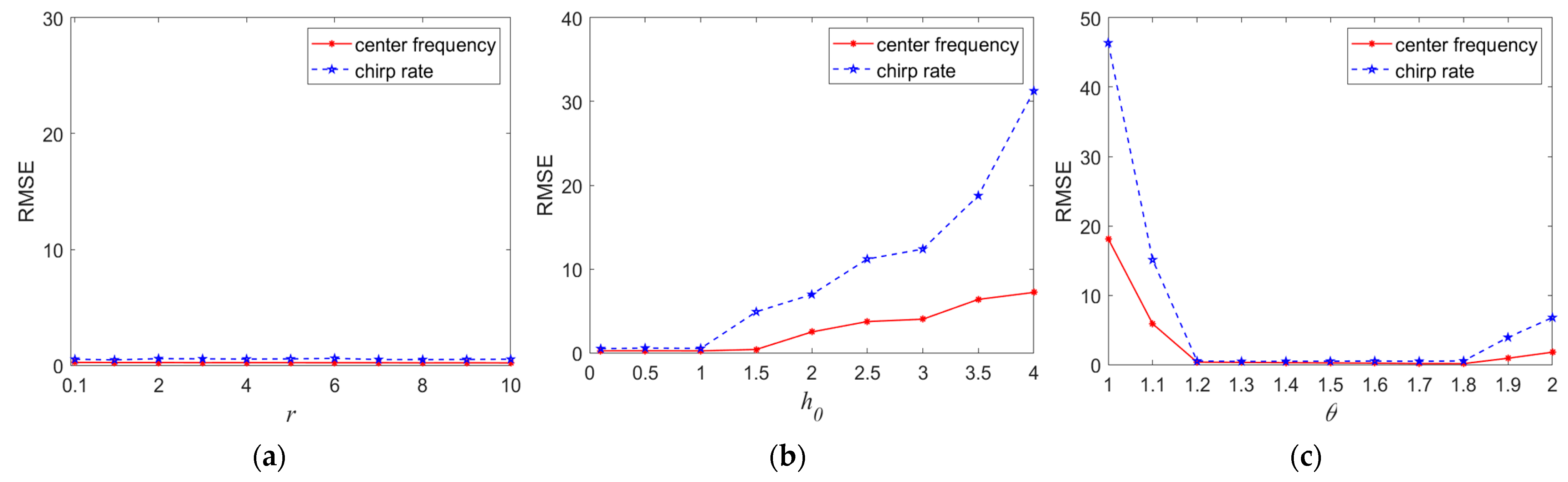
Figure 7.
The fractional spectrogram of the noisy signal (GSNR = 0 dB): (a) FTD-FRFT; (b) Sigmoid-FPSD; (c) PANT-LVD; (d) FOTD-CFRFT.
Figure 7.
The fractional spectrogram of the noisy signal (GSNR = 0 dB): (a) FTD-FRFT; (b) Sigmoid-FPSD; (c) PANT-LVD; (d) FOTD-CFRFT.
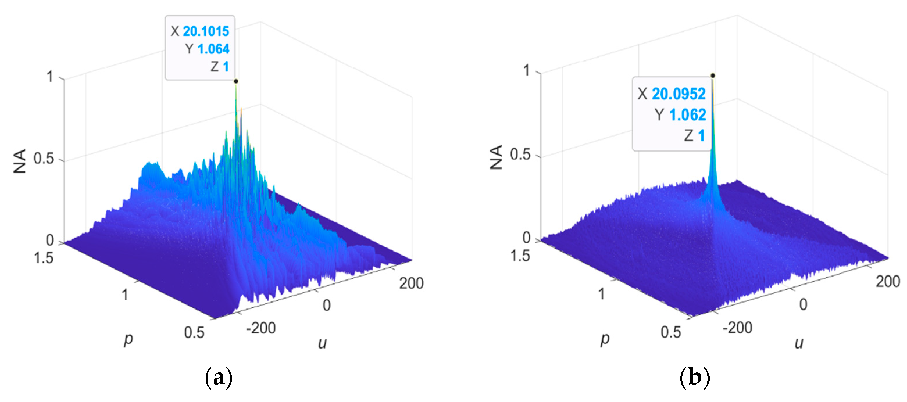

Figure 8.
The fractional spectrogram of the noisy signal () and its projection: (a) FTD-FRFT; (b) Sigmoid-FPSD; (c) PANT-LVD; (d) FOTD-CFRFT.
Figure 8.
The fractional spectrogram of the noisy signal () and its projection: (a) FTD-FRFT; (b) Sigmoid-FPSD; (c) PANT-LVD; (d) FOTD-CFRFT.
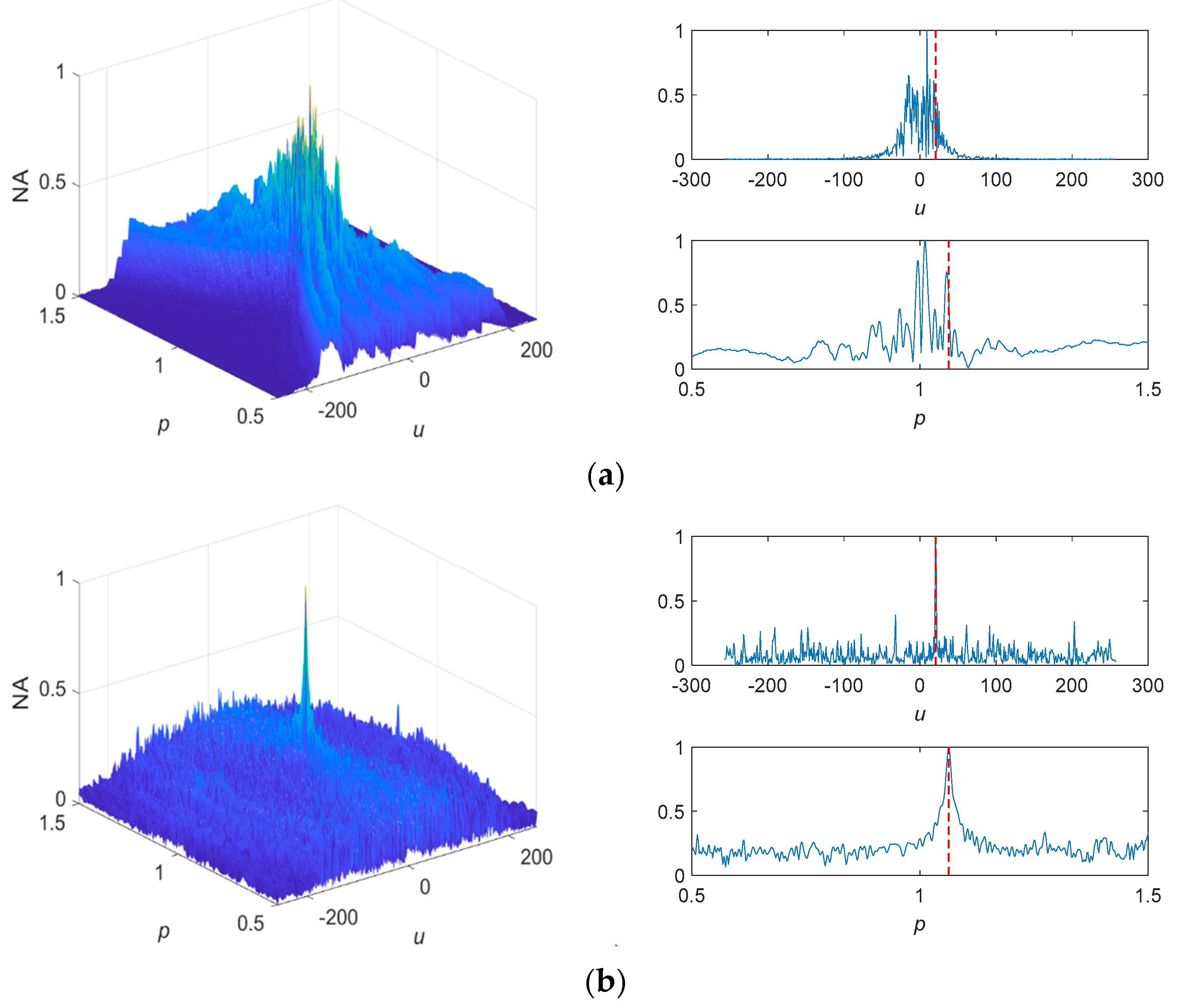

Figure 9.
RMSE of estimated parameter for four methods: (a) center frequency; (b) chirp rate. (c) center frequency (with the outlier detection algorithm); (d) chirp rate (with the outlier detection algorithm).
Figure 9.
RMSE of estimated parameter for four methods: (a) center frequency; (b) chirp rate. (c) center frequency (with the outlier detection algorithm); (d) chirp rate (with the outlier detection algorithm).

Figure 10.
The scatter diagram of estimated parameters in 100 Monte Carlo experiments (): (a) FTD-FRFT; (b) Sigmoid-FPSD; (c) PANT-LVD; (d) FOTD-CFRFT.
Figure 10.
The scatter diagram of estimated parameters in 100 Monte Carlo experiments (): (a) FTD-FRFT; (b) Sigmoid-FPSD; (c) PANT-LVD; (d) FOTD-CFRFT.


Figure 11.
RMSE of estimated parameter for different : (a) center frequency; (b) chirp rate.

Figure 12.
RMSE of center frequency and chirp rate for four methods at different : (a) center frequency; (b) chirp rate.
Figure 12.
RMSE of center frequency and chirp rate for four methods at different : (a) center frequency; (b) chirp rate.

Figure 13.
The fractional spectrum of the noisy signal when . (a) FTD-FRFT; (b) Sigmoid-FPSD; (c) PANT-LVD; (d) FOTD-CFRFT.
Figure 13.
The fractional spectrum of the noisy signal when . (a) FTD-FRFT; (b) Sigmoid-FPSD; (c) PANT-LVD; (d) FOTD-CFRFT.

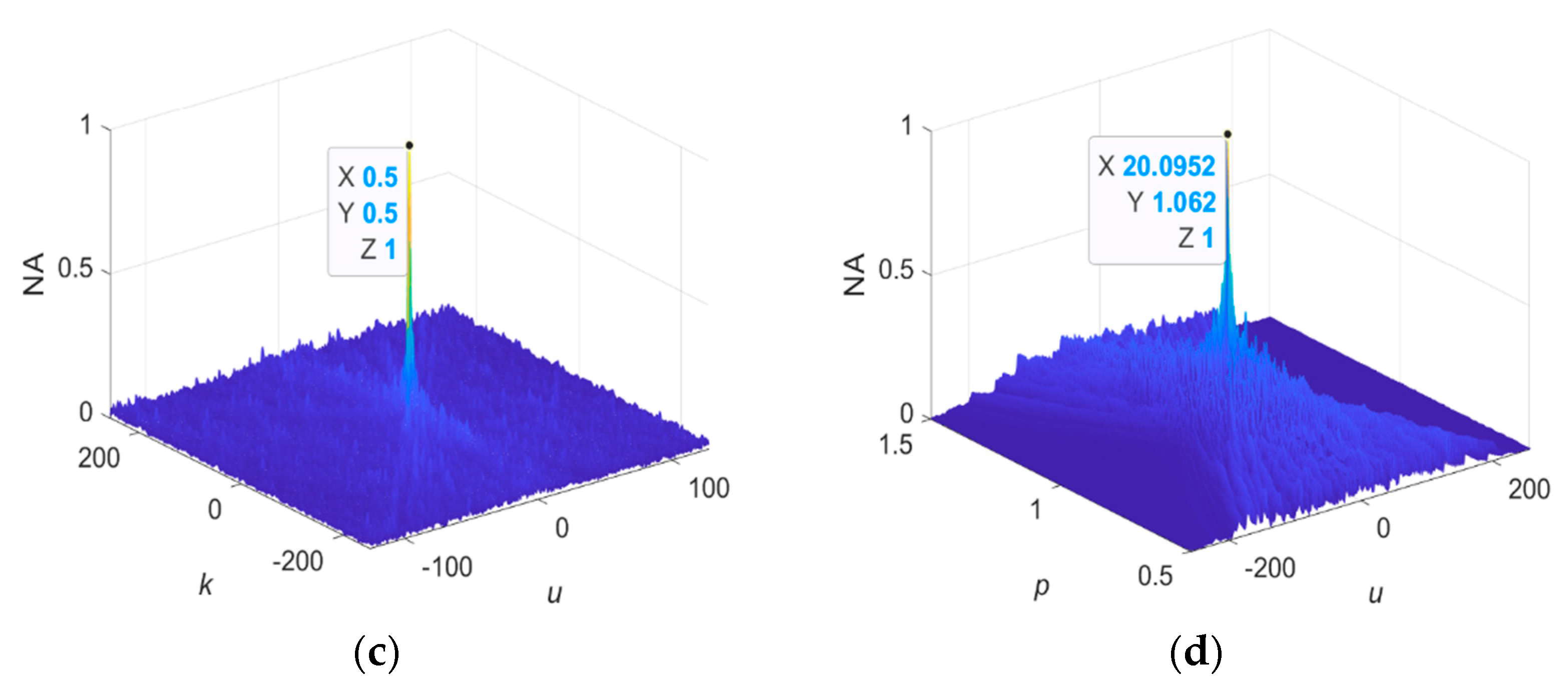
Figure 14.
RMSE of center frequency and modulation frequency for four methods at different : (a) center frequency; (b) chirp rate.
Figure 14.
RMSE of center frequency and modulation frequency for four methods at different : (a) center frequency; (b) chirp rate.

Figure 15.
The fractional spectrum of the noisy signal when . (a) FTD-FRFT; (b) Sigmoid-FPSD; (c) PANT-LVD; (d) FOTD-CFRFT.
Figure 15.
The fractional spectrum of the noisy signal when . (a) FTD-FRFT; (b) Sigmoid-FPSD; (c) PANT-LVD; (d) FOTD-CFRFT.

Figure 16.
Measured impulsive noise.

Figure 17.
The fractional spectrum of LFM signal and its projections under the weak measured impulsive noise: (a) FTD-FRFT; (b) Sigmoid-FPSD; (c) PANT-LVD; (d) FOTD-CFRFT.
Figure 17.
The fractional spectrum of LFM signal and its projections under the weak measured impulsive noise: (a) FTD-FRFT; (b) Sigmoid-FPSD; (c) PANT-LVD; (d) FOTD-CFRFT.
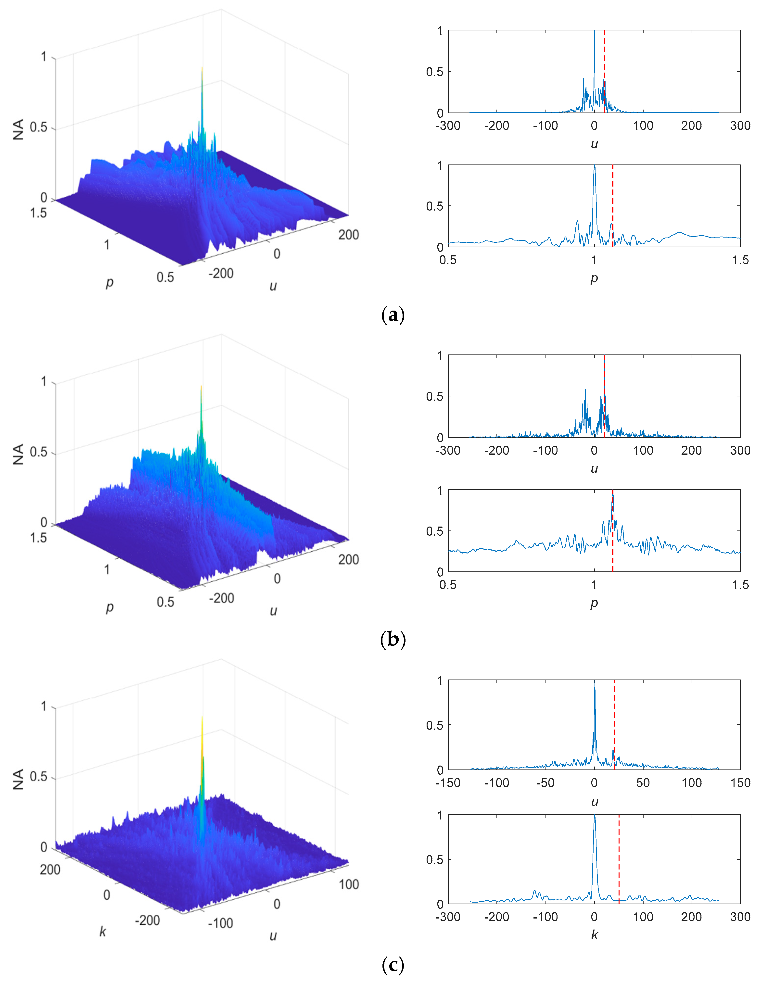
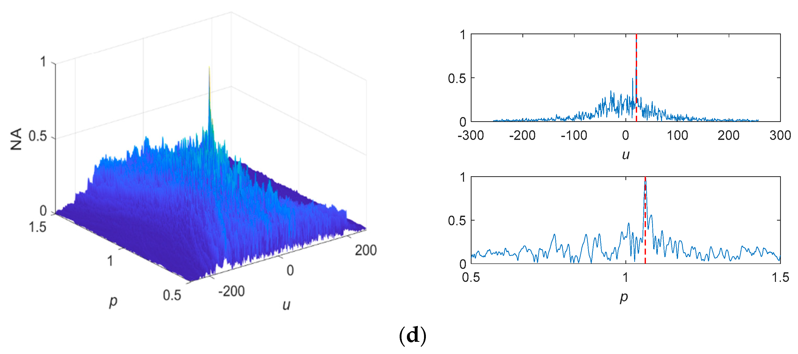
Figure 18.
The fractional spectrum of noisy signal and its projections under the strong measured impulsive noise: (a) FTD-FRFT; (b) Sigmoid-FPSD; (c) PANT-LVD; (d) FOTD-CFRFT.
Figure 18.
The fractional spectrum of noisy signal and its projections under the strong measured impulsive noise: (a) FTD-FRFT; (b) Sigmoid-FPSD; (c) PANT-LVD; (d) FOTD-CFRFT.

Table 1.
The estimate values of the center frequency and chirp rate at different GSNR.
| −6 dB | −5 dB | −4 dB | −3 dB | −2 dB | −1 dB | 0 dB | 1 dB | 2 dB | 3 dB | ||
|---|---|---|---|---|---|---|---|---|---|---|---|
| f0 | FTD-FRFT | 1.2102 | 2.2815 | 5.5838 | 7.6531 | 13.4799 | 18.5058 | 20.0341 | 20.0968 | 20.0952 | 20.0950 |
| Sigmoid-FPSD | −4.7484 | 11.7004 | 10.2649 | 20.2852 | 20.2182 | 20.1562 | 20.1863 | 20.1862 | 20.1058 | 20.1158 | |
| PANT-LVD | 16.0291 | 18.4695 | 19.6947 | 20.9199 | 20.9199 | 20.9199 | 20.9199 | 20.9199 | 20.9199 | 20.9199 | |
| FOTD-CFRFT | 20.2796 | 20.2574 | 20.2608 | 20.2617 | 20.2639 | 20.2652 | 20.2605 | 20.2603 | 20.2649 | 20.2646 | |
| k | FTD-FRFT | −3.5269 | 0.9849 | 1.3671 | 8.1601 | 25.9438 | 40.8245 | 49.4254 | 50.1678 | 50.0054 | 49.9729 |
| Sigmoid-FPSD | 45.4743 | 54.6101 | 50.1517 | 50.1191 | 50.1191 | 50.1678 | 50.1840 | 50.1677 | 50.1516 | 50.1353 | |
| PANT-LVD | 37.9866 | 43.9949 | 47.0189 | 50.1228 | 50.0730 | 50.1329 | 50.2327 | 50.2826 | 50.3425 | 50.3924 | |
| FOTD-CFRFT | 50.0982 | 50.1338 | 50.0889 | 50.1279 | 50.1832 | 50.1652 | 50.1783 | 50.1738 | 50.2006 | 50.1938 |
Disclaimer/Publisher’s Note: The statements, opinions and data contained in all publications are solely those of the individual author(s) and contributor(s) and not of MDPI and/or the editor(s). MDPI and/or the editor(s) disclaim responsibility for any injury to people or property resulting from any ideas, methods, instructions or products referred to in the content. |
© 2023 by the authors. Licensee MDPI, Basel, Switzerland. This article is an open access article distributed under the terms and conditions of the Creative Commons Attribution (CC BY) license (https://creativecommons.org/licenses/by/4.0/).
Share and Cite
MDPI and ACS Style
Wang, H.; Guo, Y.; Yang, L. Parameter Estimation of LFM Signals Based on FOTD-CFRFT under Impulsive Noise. Fractal Fract. 2023, 7, 822. https://doi.org/10.3390/fractalfract7110822
AMA Style
Wang H, Guo Y, Yang L. Parameter Estimation of LFM Signals Based on FOTD-CFRFT under Impulsive Noise. Fractal and Fractional. 2023; 7(11):822. https://doi.org/10.3390/fractalfract7110822
Chicago/Turabian StyleWang, Houyou, Yong Guo, and Lidong Yang. 2023. "Parameter Estimation of LFM Signals Based on FOTD-CFRFT under Impulsive Noise" Fractal and Fractional 7, no. 11: 822. https://doi.org/10.3390/fractalfract7110822