Improved Results on Delay-Dependent and Order-Dependent Criteria of Fractional-Order Neural Networks with Time Delay Based on Sampled-Data Control

Abstract

This paper studies the asymptotic stability of fractional-order neural networks (FONNs) with time delay utilizing a sampled-data controller. Firstly, a novel class of Lyapunov–Krasovskii functions (LKFs) is established, in which time delay and fractional-order information are fully taken into account. Secondly, by combining with the fractional-order Leibniz–Newton formula, LKFs, and other analysis techniques, some less conservative stability criteria that depend on time delay and fractional-order information are given in terms of linear matrix inequalities (LMIs). In the meantime, the sampled-data controller gain is developed under a larger sampling interval. Last, the proposed criteria are shown to be valid and less conservative than the existing ones using three numerical examples.

1. Introduction

The concept of fractional calculus was put forward almost simultaneously with the concept of integral calculus more than 300 years ago. Nevertheless, the development of fractional calculus has been somewhat slow, and it has long been studied as a purely mathematical theory due to its weak singularity and lack of precise geometric explanation and application background. Fractional calculus did not start to become a worldwide hot topic in the area of engineering applications until Mandelbrot published his work on fractal theory in 1983 [1]. With its development, it has been pointed out by experts and scholars in many fields that fractional calculus is an effective mathematical instrument for depicting real materials in terms of genetics and memory [2,3]. It is widely used in a number of distinct fields, for instance, biology, control systems, medical care, electromagnetic waves, information science, economic systems [4,5,6,7], and so on.

Artificial neural networks are a kind of network system that is constructed by imitating the microstructure of a human brain model and the research results of intelligent behavior. For the past few years, in the study of neural networks, fractional calculus has been introduced, and the FONNs model has been formed. The FONNs have two benefits over classical neural networks [8,9,10]. To begin with, their limitless memory makes them better at characterizing complicated systems and neurons, and they can also describe system models with greater accuracy. Secondly, the selection of system parameters can be made more flexible since fractional-order systems have more degrees of freedom [11]. An essential characteristic is that the fractional-order derivative depends on an infinite number of terms, whereas the integer-order derivative only represents a finite series. Because of this, the integer-order derivative is a local operator, whereas the fractional-order derivative has the memory of all previous occurrences. Therefore, the dynamic analysis of FONNs has attracted great interest among scholars, and a wealth of results have emerged. For example, the synchronization problem of fractional-order complex-valued neural networks with delay was discussed by employing the linear feedback control and comparison theorem of fractional-order linear delay systems [12]. A crucial finding of Caputo’s fractional-order derivative of a quadratic function was used to study the issue of robust finite-time guaranteed cost control for FONNs, which is based on finite-time stability theory [13]. With the use of fractional calculus and the fractional-order Razumikhin theorem, the passivity of uncertain FONNs with time-varying delay was investigated [14].

Effective control methods are very important from the viewpoint of the control strategy for the analysis of FONNs with complex nonlinear dynamical characteristics, such as sliding mode control [15,16,17], impulsive control [17,18,19], state feedback control [20,21], and sampled-data control [22,23,24,25]. It is important to note that sampled-data control, when compared with other control strategies, can successfully reduce control costs and significantly increase the controller’s usability and utilization. It is common knowledge that a longer sample interval has benefits such as fewer controller drivers, less signal transmission, and less communication channel utilization. An important problem in the study of FONNs stability with the sampled-data controller is how to obtain a longer sampling period. Referencing [26], fractional-order Razumikhin theorem and LMI were used to provide stability conditions for input delay dependence and order dependence. A sampled-data controller was proposed in accordance with the stability requirement. The findings from the studies mentioned above are still conservative; therefore, much work needs to be carried out in this area. So, the question of how to obtain the FONNs stability conditions with low conservatism is crucial. On the other hand, the time delay’s presence [27,28,29] makes the analysis and synthesis of the system more complicated and difficult and also leads to the deterioration of system performance and even instability. Hence, it has significant theoretical implications for studying the stability of FONNs with time delay via sampled-data control.

Inspired by the aforementioned comments, this paper focuses on the controller design issue of FONNs with time delay using a new method. The findings of this study can serve as a foundation and source of encouragement for the development of FONNs with time-delay theory. The innovations in this paper are as follows:

•

A novel class of LKFs is established, in which time delay and fractional-order information are taken into account so as to reduce the conservatism of the stability criteria.

•

A new method is proposed to present the relations among the terms of the fractional-order Leibniz–Newton formula for FONNs with time delay by free-weighting matrices. Because $-\frac{\varpi }{\Gamma \left(\delta \right)}{\int }_{t-\varpi }^t{(t-u)}^{\delta -1}{\left({}_{t_0}^C{D}_u^{\delta }\xi \left(u\right)\right)}^{T}W\left({}_{t_0}^C{D}_u^{\delta }\xi \left(u\right)\right)du$ is very difficult to deal with, more functionals need to be constructed, which may also be conservative and computationally complex. Based on this method, the estimation of $-\frac{\varpi }{\Gamma \left(\delta \right)}{\int }_{t-\varpi }^t{(t-u)}^{\delta -1}\times {\left({}_{t_0}^C{D}_u^{\delta }\xi \left(u\right)\right)}^{T}W\left({}_{t_0}^C{D}_u^{\delta }\xi \left(u\right)\right)du$ can be avoided.

•

Compared with the existing results, a less conservative stability for FONNs is established, which achieves a longer sampling period. Moreover this method is applied to the stability analysis of fractional-order linear time-delay systems.

•

Based on the stability criteria obtained, the sampled-data controller of the FONNs is designed. The results are in terms of LMIs, which make computation and application easier.

The structure of this paper is as follows: In Section 2, the definitions, assumptions, and lemmas required for the FONNs with time delay to be stable are provided. The asymptotic stability conditions of FONNs with time delay are put forth, and a sampled-data controller is designed in Section 3. Two numerical examples validate the rationality of the theoretical method in Section 4. Section 5 summarizes the work of this paper.

2. Preliminaries

Definition 1

([5]). The $\delta \in (0,1)$ -order Caputo fractional-order derivative for function $\widehat{y}\left(v\right)$ is

$$\begin{array}{c}\hfill {}_{t_0}^{\mathcal{C}}{\mathcal{D}}_v^{\delta }\widehat{y}\left(v\right)=\frac{1}{\Gamma (m-\delta )}{\int }_{t_0}^v\frac{{\widehat{y}}^{\left(m\right)}\left(\gamma \right)}{{(v-\gamma )}^{\delta -m+1}}d\gamma ,\end{array}$$

where $m=\left[\delta \right]+1$, $\Gamma (·)$ is the Gamma function, $\widehat{y}\left(v\right)\in C^m([t_0,\infty ),{\Re }^n)$.

Definition 2

([5]). For an integrable function $\widehat{y}\left(v\right):[t_0,\infty )\to {\Re }^n$, the fractional-order integral of order $\delta \in {\Re }_{+}$ is given below.

$$\begin{array}{c}\hfill {}_{t_0}{I}_v^{\delta }\widehat{y}\left(v\right)=\frac{1}{\Gamma \left(\delta \right)}{\int }_{t_0}^v{(v-\gamma )}^{\delta -1}\widehat{y}\left(\gamma \right)d\gamma .\end{array}$$

Lemma 1

([5,30]). Some properties of the fractional-order integral and derivative:

• For any $t_0\in [0,\infty ),\widehat{y}\left(v\right)\in C^1([0,\infty ),\Re )$ and $\delta \in (0,1)$, ${}_{t_0}^{\mathcal{C}}{\mathcal{D}}_v^{\delta }{(}_{t_0}{I}_v^{\delta }\widehat{y}\left(v\right))=\widehat{y}\left(v\right).$
• For any $t_0\in [0,\infty ),\widehat{y}\left(v\right)\in C^1([0,\infty ),\Re )$ and $\delta \in (0,1)$, ${}_{t_0}{I}_v^{\delta }{(}_{t_0}^{\mathcal{C}}{\mathcal{D}}_v^{\delta }\widehat{y}\left(v\right))=\widehat{y}\left(v\right)-\widehat{y}\left(t_0\right).$
• ${}_{t_0}^{\mathcal{C}}{\mathcal{D}}_v^{\delta }\left({\widehat{y}}^T\left(v\right)\stackrel{⌢}{Y}\widehat{y}\left(v\right)\right)\le 2{\widehat{y}}^T\left(v\right)\stackrel{⌢}{Y}\left({}_{t_0}^{\mathcal{C}}{\mathcal{D}}_v^{\delta }\widehat{y}\left(v\right)\right)$, for any $\widehat{y}\left(v\right)\in {\Re }^n$, where $\delta \in (0,1)$, $\stackrel{⌢}{Y}$ is symmetric positive definite matrix.

Lemma 2

([31]). If the symmetric matrix $\stackrel{⌢}{\mathcal{Q}}>0$, for any $\widehat{y}\left(v\right)\in C^1([t_0,v],{\Re }^n)$, the following inequality is true:

$${}_{t_0}{I}_v^{\delta }{\widehat{y}}^T\left(v\right)\stackrel{⌢}{\mathcal{Q}}\widehat{y}\left(v\right)\ge \frac{\Gamma (\delta +1)}{{(v-t_0)}^{\delta }}{\left({}_{t_0}{I}_v^{\delta }\widehat{y}\left(v\right)\right)}^T\stackrel{⌢}{\mathcal{Q}}\left({}_{t_0}{I}_v^{\delta }\widehat{y}\left(v\right)\right).$$

Lemma 3

([32]). The matrix $\wp =\left[\begin{array}{cc}{\wp }_{11}& {\wp }_{12}\\ \ast & {\wp }_{22}\end{array}\right]<0$, if and only if equivalent (1) or (2) holds:

• ${\wp }_{11}<0,{\wp }_{22}-{\wp }_{12}^T{\wp }_{11}^{-1}{\wp }_{12}<0$;
• ${\wp }_{22}<0,{\wp }_{11}-{\wp }_{12}{\wp }_{22}^{-1}{\wp }_{12}^T<0$.

Consider the following FONNs with time delay

$$\begin{array}{c}\hfill \left\{\begin{array}{c}{}_{t_0}^C{D}_t^{\delta }\xi \left(t\right)=A\xi \left(t\right)+Bf\left(\xi \left(t\right)\right)+C\xi (t-\sigma )+u\left(t\right),\hfill \\ \xi \left(t\right)=\psi \left(t\right),t\in [-\sigma ,0]\hfill \end{array}\right.\end{array}$$

(1)

where $\xi \left(t\right)={({\xi }_1\left(t\right),\cdots ,{\xi }_n\left(t\right))}^T\in {\Re }^n$, $f\left(\xi \left(t\right)\right)={(f_1\left({\xi }_1\left(t\right)\right),\cdots ,f_n\left({\xi }_n\left(t\right)\right))}^T\in {\Re }^n$, and $u\left(t\right)={(u_1\left(t\right),\cdots ,u_n\left(t\right))}^T$ stand for state, activation function, and control input; the fractional-order $\delta \in (0,1)$; $\sigma$ is constant time delay; and $A\in {\Re }^n$, $B\in {\Re }^n$, $C\in {\Re }^n$ are known constant matrices. $\psi \left(t\right)$ denotes the initial condition.

To reduce data transfers as much as possible while maintaining the required control in terms of performance for the stability of the model (1), we developed a sampled-data controller. Accordingly, the sampled-data controller is depicted below:

$$\begin{array}{c}\hfill u\left(t\right)=K\xi \left(t_{\ell }\right),\end{array}$$

(2)

where K is the control gain to be designed. In this paper, the control signal is generated via a zero-order holder (ZOH) function at the sampling moments $0=t_0\le t_1\le \cdots \le \underset{\ell \to +\infty }{lim}{t}_{\ell }=+\infty$. For any integer $\ell >0$, the variable sampling intervals are defined as $0<t_{\ell +1}-t_{\ell }={\varpi }_{\ell }\le \varpi$, where $\varpi$ is the upper bound on the sampling periods.

Bringing (2) into (1), then using the input time-varying delay approach, we obtain

$$\begin{array}{c}\hfill {}_{t_0}^C{D}_t^{\delta }\xi \left(t\right)=A\xi \left(t\right)+Bf(\xi \left(t\right)+C\xi (t-\sigma ))+K\xi (t-\varpi \left(t\right)),t>0,\end{array}$$

(3)

where $\varpi \left(t\right)=t-t_{\ell },t\in [t_{\ell },t_{\ell +1}]$. It is simple to understand $\varpi \left(t\right)\le {\varpi }_{\ell }<\varpi$.

We require the following assumption before moving on:

Assumption 1.

The activation functions $f_i(·)(i=1,2,\cdots ,n)$ are continuous and fulfill

$$\begin{array}{c}\hfill l_i^{-}<\frac{f_i\left({\varsigma }_1\right)-f_i\left({\varsigma }_2\right)}{{\varsigma }_1-{\varsigma }_2}<l_i^{+},{\varsigma }_1\ne {\varsigma }_2\in \Re ,\end{array}$$

(4)

where $l_i^{-}$ and $l_i^{+}$ are constants.

3. Main Results

We talk about the stability of the model (3) through the sampled-data controller (2) in this Section. The following theorem presents the LMIs for the delay-dependent and order-dependent stability criterion for the model (3).

Theorem 1.

For the given parameters $\varpi \ge 0$, $\sigma \ge 0$, and matrix K, the model (3) is asymptotically stable, if there exist symmetric matrices $P>0$, $Q>0$, $M>0$, $E>0$, diagonal matrix $W_1>0$, symmetric matrices $W\ge 0$, $H\ge 0$, ${\Xi }_{ii}\ge 0$, ${\Im }_{ii}\ge 0(i=1,2,3)$, any matrices $S_i$, $N_i(i=1,2,3)$, ${\Xi }_{ij}$, and ${\Im }_{ij}(1\le i<j\le 3)$ such that the following LMIs hold:

$$\begin{array}{c}\hfill {{\rm Y}}_1=\left[\begin{array}{ccc}{\Im }_{11}& {\Im }_{12}& {\Im }_{13}\\ \ast & {\Im }_{22}& {\Im }_{23}\\ \ast & \ast & {\Im }_{33}\end{array}\right]\ge 0,\end{array}$$

(5)

$$\begin{array}{c}\hfill {{\rm Y}}_2=\left[\begin{array}{cccc}{\Im }_{11}& {\Im }_{12}& {\Im }_{13}& N_1\\ \ast & {\Im }_{22}& {\Im }_{23}& N_2\\ \ast & \ast & {\Im }_{33}& N_3\\ \ast & \ast & \ast & W\end{array}\right]\ge 0,\end{array}$$

(6)

$$\begin{array}{c}\hfill {{\rm Y}}_3=\left[\begin{array}{cccc}{\Xi }_{11}& {\Xi }_{12}& {\Xi }_{13}& S_1\\ \ast & {\Xi }_{22}& {\Xi }_{23}& S_2\\ \ast & \ast & {\Xi }_{33}& S_3\\ \ast & \ast & \ast & H\end{array}\right]\ge 0,\end{array}$$

(7)

$$\begin{array}{c}\hfill {{\rm Y}}_4=\left[\begin{array}{cccccc}{\aleph }_{1,1}& {\aleph }_{1,2}& {\aleph }_{1,3}& {\aleph }_{1,4}& {\aleph }_{1,5}& {\aleph }_{1,6}\\ \ast & {\aleph }_{2,2}& {\aleph }_{2,3}& {\aleph }_{2,4}& 0& {\aleph }_{2,6}\\ \ast & \ast & {\aleph }_{3,3}& 0& {\aleph }_{3,5}& {\aleph }_{3,6}\\ \ast & \ast & \ast & {\aleph }_{4,4}& 0& 0\\ \ast & \ast & \ast & \ast & {\aleph }_{5,5}& 0\\ \ast & \ast & \ast & \ast & \ast & {\aleph }_{6,6}\end{array}\right]<0,\end{array}$$

(8)

where

$$\begin{array}{cc}\hfill {\aleph }_{1,1}& =PA+A^{T}P+Q+\frac{{\varpi }^{\delta +1}}{\Gamma (\delta +1)}{A}^{T}WA+\frac{{\varpi }^{\delta +1}}{\Gamma (\delta +1)}{A}^{T}MA+\frac{{\sigma }^{\delta +1}}{\Gamma (\delta +1)}{A}^{T}HA\hfill \\ \hfill & +\frac{{\sigma }^{\delta +1}}{\Gamma (\delta +1)}{A}^{T}EA+\varpi N_1+\varpi N_1^T+\sigma S_1+\sigma S_1^T+\frac{{\varpi }^{\delta +1}}{\Gamma (\delta +1)}{\Im }_{11}+\frac{{\sigma }^{\delta +1}}{\Gamma (\delta +1)}{\Xi }_{11}\hfill \\ \hfill & +L^T{W}_{1}L,\hfill \end{array}$$

$$\begin{array}{cc}\hfill {\aleph }_{1,2}& =PK+\frac{{\varpi }^{\delta +1}}{\Gamma (\delta +1)}{A}^{T}WK+\frac{{\varpi }^{\delta +1}}{\Gamma (\delta +1)}{A}^{T}MK+\frac{{\sigma }^{\delta +1}}{\Gamma (\delta +1)}{A}^{T}HK+\frac{{\sigma }^{\delta +1}}{\Gamma (\delta +1)}{A}^{T}EK\hfill \\ \hfill & -\varpi N_1+\varpi N_2^T+\frac{{\varpi }^{\delta +1}}{\Gamma (\delta +1)}{\Im }_{12},\hfill \\ \hfill {\aleph }_{1,3}& =PC+\frac{{\varpi }^{\delta +1}}{\Gamma (\delta +1)}{A}^{T}WC+\frac{{\varpi }^{\delta +1}}{\Gamma (\delta +1)}{A}^{T}MC+\frac{{\sigma }^{\delta +1}}{\Gamma (\delta +1)}{A}^{T}HC+\frac{{\sigma }^{\delta +1}}{\Gamma (\delta +1)}{A}^{T}EC\hfill \\ \hfill & -\sigma S_1+\sigma S_2^T+\frac{{\sigma }^{\delta +1}}{\Gamma (\delta +1)}{\Xi }_{12},\hfill \\ \hfill {\aleph }_{1,4}& =\varpi N_1+\varpi N_3^T+\frac{{\varpi }^{\delta +1}}{\Gamma (\delta +1)}{\Im }_{13},{\aleph }_{1,5}=\sigma S_1+\sigma S_3^T+\frac{{\sigma }^{\delta +1}}{\Gamma (\delta +1)}{\Xi }_{13},\hfill \\ \hfill {\aleph }_{1,6}& =PB+\frac{{\varpi }^{\delta +1}}{\Gamma (\delta +1)}{A}^{T}WB+\frac{{\varpi }^{\delta +1}}{\Gamma (\delta +1)}{A}^{T}MB+\frac{{\sigma }^{\delta +1}}{\Gamma (\delta +1)}{A}^{T}HB+\frac{{\sigma }^{\delta +1}}{\Gamma (\delta +1)}{A}^{T}EB,\hfill \\ \hfill {\aleph }_{2,2}& =\frac{{\varpi }^{\delta +1}}{\Gamma (\delta +1)}{K}^{T}WK+\frac{{\varpi }^{\delta +1}}{\Gamma (\delta +1)}{K}^{T}MK+\frac{{\sigma }^{\delta +1}}{\Gamma (\delta +1)}{K}^{T}HK+\frac{{\sigma }^{\delta +1}}{\Gamma (\delta +1)}{K}^{T}EK\hfill \\ \hfill & -\varpi N_2-\varpi N_2^T+\frac{{\varpi }^{\delta +1}}{\Gamma (\delta +1)}{\Im }_{22},\hfill \\ \hfill {\aleph }_{2,3}& =\frac{{\varpi }^{\delta +1}}{\Gamma (\delta +1)}{K}^{T}WC+\frac{{\varpi }^{\delta +1}}{\Gamma (\delta +1)}{K}^{T}MC+\frac{{\sigma }^{\delta +1}}{\Gamma (\delta +1)}{K}^{T}HC+\frac{{\sigma }^{\delta +1}}{\Gamma (\delta +1)}{K}^{T}EC,\hfill \\ \hfill {\aleph }_{2,4}& =\varpi N_2-\varpi N_3^T+\frac{{\varpi }^{\delta +1}}{\Gamma (\delta +1)}{\Im }_{23},\hfill \\ \hfill {\aleph }_{2,6}& =\frac{{\varpi }^{\delta +1}}{\Gamma (\delta +1)}{K}^{T}WB+\frac{{\varpi }^{\delta +1}}{\Gamma (\delta +1)}{K}^{T}MB+\frac{{\sigma }^{\delta +1}}{\Gamma (\delta +1)}{K}^{T}HB+\frac{{\sigma }^{\delta +1}}{\Gamma (\delta +1)}{K}^{T}EB,\hfill \\ \hfill {\aleph }_{3,3}& =-Q+\frac{{\varpi }^{\delta +1}}{\Gamma (\delta +1)}{C}^{T}WC+\frac{{\varpi }^{\delta +1}}{\Gamma (\delta +1)}{C}^{T}MC+\frac{{\sigma }^{\delta +1}}{\Gamma (\delta +1)}{C}^{T}HC+\frac{{\sigma }^{\delta +1}}{\Gamma (\delta +1)}{C}^{T}EC\hfill \\ \hfill & -\sigma S_2-\sigma S_2^T+\frac{{\sigma }^{\delta +1}}{\Gamma (\delta +1)}{\Xi }_{22},\hfill \\ \hfill {\aleph }_{3,5}& =\sigma S_2-\sigma S_3^T+\frac{{\sigma }^{\delta +1}}{\Gamma (\delta +1)}{\Xi }_{23},\hfill \\ \hfill {\aleph }_{3,6}& =\frac{{\varpi }^{\delta +1}}{\Gamma (\delta +1)}{C}^{T}WB+\frac{{\varpi }^{\delta +1}}{\Gamma (\delta +1)}{C}^{T}MB+\frac{{\sigma }^{\delta +1}}{\Gamma (\delta +1)}{C}^{T}HB+\frac{{\sigma }^{\delta +1}}{\Gamma (\delta +1)}{C}^{T}EB,\hfill \\ \hfill {\aleph }_{4,4}& =-\frac{\Gamma (\delta +1)}{{\varpi }^{\delta -1}}M+\varpi N_3+\varpi N_3^T+\frac{{\varpi }^{\delta +1}}{\Gamma (\delta +1)}{\Im }_{33},\hfill \\ \hfill {\aleph }_{5,5}& =-\frac{\Gamma (\delta +1)}{{\sigma }^{\delta -1}}E+\sigma S_3+\sigma S_3^T+\frac{{\sigma }^{\delta +1}}{\Gamma (\delta +1)}{\Xi }_{33},\hfill \\ \hfill {\aleph }_{6,6}& =\frac{{\varpi }^{\delta +1}}{\Gamma (\delta +1)}{B}^{T}WB+\frac{{\varpi }^{\delta +1}}{\Gamma (\delta +1)}{B}^{T}MB+\frac{{\sigma }^{\delta +1}}{\Gamma (\delta +1)}{B}^{T}HB+\frac{{\sigma }^{\delta +1}}{\Gamma (\delta +1)}{B}^{T}EB-W_1.\hfill \end{array}$$

Proof. 

For ease of use, we denote as

$$\begin{array}{cc}\hfill y\left(u\right)& =\frac{1}{\Gamma (1-\delta )}{\int }_{t_0}^{t-\varpi \left(t\right)}{(u-s)}^{-\delta }\dot{\xi }\left(s\right)ds,p\left(u\right)=\frac{1}{\Gamma (1-\delta )}{\int }_{t_0}^{t-\sigma }{(u-s)}^{-\delta }\dot{\xi }\left(s\right)ds.\hfill \end{array}$$

(9)

Then, select the LKFs listed below:

$$\begin{array}{c}\hfill V_1\left(\xi \left(t\right)\right)={}_{t_0}^C{D}_t^{-(1-\delta )}\left({\xi }^T\left(t\right)P\xi \left(t\right)\right),\end{array}$$

(10)

$$\begin{array}{c}\hfill V_2\left(\xi \left(t\right)\right)={\int }_{t-\sigma }^t{\xi }^T\left(s\right)Q\xi \left(s\right)ds,\end{array}$$

(11)

$$\begin{array}{c}\hfill V_3\left(\xi \left(t\right)\right)=\frac{\varpi }{\Gamma \left(\delta \right)}{\int }_{-\varpi }^0{(-\vartheta )}^{\delta -1}{\int }_{t+\vartheta }^t{\left({}_{t_0}^C{D}_s^{\delta }\xi \left(s\right)\right)}^{T}W\left({}_{t_0}^C{D}_s^{\delta }\xi \left(s\right)\right)dsd\vartheta ,\end{array}$$

(12)

$$\begin{array}{c}\hfill V_4\left(\xi \left(t\right)\right)=\frac{\sigma }{\Gamma \left(\delta \right)}{\int }_{-\sigma }^0{(-\vartheta )}^{\delta -1}{\int }_{t+\vartheta }^t{\left({}_{t_0}^C{D}_s^{\delta }\xi \left(s\right)\right)}^{T}H\left({}_{t_0}^C{D}_s^{\delta }\xi \left(s\right)\right)dsd\vartheta ,\end{array}$$

(13)

$$\begin{array}{c}\hfill V_5\left(\xi \left(t\right)\right)=\frac{\varpi }{\Gamma \left(\delta \right)}{\int }_{-\varpi }^0{(-\vartheta )}^{\delta -1}{\int }_{t+\vartheta }^t{y}^T\left(s\right)My\left(s\right)dsd\vartheta ,\end{array}$$

(14)

$$\begin{array}{c}\hfill V_6\left(\xi \left(t\right)\right)=\frac{\sigma }{\Gamma \left(\delta \right)}{\int }_{-\sigma }^0{(-\vartheta )}^{\delta -1}{\int }_{t+\vartheta }^t{p}^T\left(s\right)Ep\left(s\right)dsd\vartheta .\end{array}$$

(15)

The time derivative of $V_i\left(\xi \left(t\right)\right)(i=1,2,3\cdots ,6)$ according to model (3) is given by

$$\begin{array}{c}\hfill {\dot{V}}_1\left(\xi \left(t\right)\right)={}_{t_0}^C{D}_t^{\delta }\left({\xi }^T\left(t\right)P\xi \left(t\right)\right),\end{array}$$

(16)

as stated by Lemma 1, one has

$$\begin{array}{cc}\hfill {}_{t_0}^C{D}_t^{\delta }\left({\xi }^T\left(t\right)P\xi \left(t\right)\right)& \le 2{\xi }^T\left(t\right)P{}_{t_0}^C{D}_t^{\delta }\left(\xi \left(t\right)\right)\hfill \\ \hfill & =2{\xi }^T\left(t\right)P(A\xi \left(t\right)+Bf\left(\xi \left(t\right)\right)+C\xi (t-\sigma )+K\xi (t-\varpi \left(t\right))),\hfill \end{array}$$

(17)

and ${\dot{V}}_2\left(\xi \left(t\right)\right)$, ${\dot{V}}_3\left(\xi \left(t\right)\right)$ can be computed as

$$\begin{array}{c}\hfill {\dot{V}}_2\left(\xi \left(t\right)\right)={\xi }^T\left(t\right)Q\xi \left(t\right)-{\xi }^T(t-\sigma )Q\xi (t-\sigma ),\end{array}$$

(18)

$$\begin{array}{cc}\hfill {\dot{V}}_3\left(\xi \left(t\right)\right)& =\frac{\varpi }{\Gamma \left(\delta \right)}{\int }_{-\varpi }^0{(-\vartheta )}^{\delta -1}{\left({}_{t_0}^C{D}_t^{\delta }\xi \left(t\right)\right)}^{T}W\left({}_{t_0}^C{D}_t^{\delta }\xi \left(t\right)\right)d\vartheta \hfill \\ \hfill & -\frac{\varpi }{\Gamma \left(\delta \right)}{\int }_{-\varpi }^0{(-\vartheta )}^{\delta -1}{\left({}_{t_0}^C{D}_{t+\vartheta }^{\delta }\xi (t+\vartheta )\right)}^{T}W\left({}_{t_0}^C{D}_{t+\vartheta }^{\delta }\xi (t+\vartheta )\right)d\vartheta \hfill \\ \hfill & =\frac{{\varpi }^{\delta +1}}{\Gamma (\delta +1)}{\left({}_{t_0}^C{D}_t^{\delta }\xi \left(t\right)\right)}^{T}W\left({}_{t_0}^C{D}_t^{\delta }\xi \left(t\right)\right)\hfill \\ \hfill & -\frac{\varpi }{\Gamma \left(\delta \right)}{\int }_{t-\varpi }^t{(t-u)}^{\delta -1}{\left({}_{t_0}^C{D}_u^{\delta }\xi \left(u\right)\right)}^{T}W\left({}_{t_0}^C{D}_u^{\delta }\xi \left(u\right)\right)du,\hfill \end{array}$$

(19)

according to model (3), we can obtain $\varpi \left(t\right)<\varpi$, so one has

$$\begin{array}{cc}\hfill {\dot{V}}_3\left(\xi \left(t\right)\right)& \le \frac{{\varpi }^{\delta +1}}{\Gamma (\delta +1)}{\left({}_{t_0}^C{D}_t^{\delta }\xi \left(t\right)\right)}^{T}W\left({}_{t_0}^C{D}_t^{\delta }\xi \left(t\right)\right)\hfill \\ \hfill & -\frac{\varpi }{\Gamma \left(\delta \right)}{\int }_{t-\varpi \left(t\right)}^t{(t-u)}^{\delta -1}{\left({}_{t_0}^C{D}_u^{\delta }\xi \left(u\right)\right)}^{T}W\left({}_{t_0}^C{D}_u^{\delta }\xi \left(u\right)\right)du\hfill \end{array}$$

$$\begin{array}{cc}\hfill & =\frac{{\varpi }^{\delta +1}}{\Gamma (\delta +1)}{(A\xi \left(t\right)+Bf\left(\xi \left(t\right)\right)+C\xi (t-\sigma )+K\xi (t-\varpi \left(t\right)))}^{T}W\hfill \\ \hfill & \times \left(A\xi \right(t)+Bf(\xi \left(t\right))+C\xi (t-\sigma )+K\xi (t-\varpi \left(t\right)\left)\right)\hfill \\ \hfill & -\frac{\varpi }{\Gamma \left(\delta \right)}{\int }_{t-\varpi \left(t\right)}^t{(t-u)}^{\delta -1}{\left({}_{t-\varpi \left(t\right)}^C{D}_u^{\delta }\xi \left(u\right)+y\left(u\right)\right)}^{T}W\left({}_{t-\varpi \left(t\right)}^C{D}_u^{\delta }\xi \left(u\right)+y\left(u\right)\right)du,\hfill \end{array}$$

(20)

we can obtain the derivative of $V_4\left(\xi \left(t\right)\right)$ as

$$\begin{array}{cc}\hfill {\dot{V}}_4\left(\xi \left(t\right)\right)& =\frac{\sigma }{\Gamma \left(\delta \right)}{\int }_{-\sigma }^0{(-\vartheta )}^{\delta -1}{\left({}_{t_0}^C{D}_t^{\delta }\xi \left(t\right)\right)}^{T}H\left({}_{t_0}^C{D}_t^{\delta }\xi \left(t\right)\right)d\vartheta \hfill \\ \hfill & -\frac{\sigma }{\Gamma \left(\delta \right)}{\int }_{-\sigma }^0{(-\vartheta )}^{\delta -1}{\left({}_{t_0}^C{D}_{t+\vartheta }^{\delta }\xi (t+\vartheta )\right)}^{T}H\left({}_{t_0}^C{D}_{t+\vartheta }^{\delta }\xi (t+\vartheta )\right)d\vartheta \hfill \\ \hfill & =\frac{{\sigma }^{\delta +1}}{\Gamma (\delta +1)}{\left({}_{t_0}^C{D}_t^{\delta }\xi \left(t\right)\right)}^{T}H\left({}_{t_0}^C{D}_t^{\delta }\xi \left(t\right)\right)\hfill \\ \hfill & -\frac{\sigma }{\Gamma \left(\delta \right)}{\int }_{t-\sigma }^t{(t-u)}^{\delta -1}{\left({}_{t_0}^C{D}_u^{\delta }\xi \left(u\right)\right)}^{T}H\left({}_{t_0}^C{D}_u^{\delta }\xi \left(u\right)\right)du\hfill \\ \hfill & =\frac{{\sigma }^{\delta +1}}{\Gamma (\delta +1)}{(A\xi \left(t\right)+Bf\left(\xi \left(t\right)\right)+C\xi (t-\sigma )+K\xi (t-\varpi \left(t\right)))}^{T}H\hfill \\ \hfill & \times \left(A\xi \right(t)+Bf(\xi \left(t\right))+C\xi (t-\sigma )+K\xi (t-\varpi \left(t\right)\left)\right)\hfill \\ \hfill & -\frac{\sigma }{\Gamma \left(\delta \right)}{\int }_{t-\sigma }^t{(t-u)}^{\delta -1}{\left({}_{t-\sigma }^C{D}_u^{\delta }\xi \left(u\right)+p\left(u\right)\right)}^{T}H\left({}_{t-\sigma }^C{D}_u^{\delta }\xi \left(u\right)+p\left(u\right)\right)du,\hfill \end{array}$$

(21)

on the basis of Lemma 1, the ${\dot{V}}_3\left(\xi \left(t\right)\right),{\dot{V}}_4\left(\xi \left(t\right)\right)$ are equal to

$$\begin{array}{cc}\hfill {\dot{V}}_3\left(\xi \left(t\right)\right)& =\frac{{\varpi }^{\delta +1}}{\Gamma (\delta +1)}{(A\xi \left(t\right)+Bf\left(\xi \left(t\right)\right)+C\xi (t-\sigma )+K\xi (t-\varpi \left(t\right)))}^{T}W\hfill \\ \hfill & \times \left(A\xi \right(t)+Bf(\xi \left(t\right))+C\xi (t-\sigma )+K\xi (t-\varpi \left(t\right)\left)\right)\hfill \\ \hfill & -\frac{\varpi }{\Gamma \left(\delta \right)}{\int }_{t-\varpi \left(t\right)}^t{(t-u)}^{\delta -1}{\left({}_{t-\varpi \left(t\right)}^C{D}_u^{\delta }(\xi \left(u\right)+{}_{t-\varpi \left(t\right)}{I}_u^{\delta }y\left(u\right))\right)}^{T}W\hfill \\ \hfill & \times \left({}_{t-\varpi \left(t\right)}^C{D}_u^{\delta }(\xi \left(u\right)+{}_{t-\varpi \left(t\right)}{I}_u^{\delta }y\left(u\right))\right)du,\hfill \end{array}$$

(22)

$$\begin{array}{cc}\hfill {\dot{V}}_4\left(\xi \left(t\right)\right)& =\frac{{\sigma }^{\delta +1}}{\Gamma (\delta +1)}{(A\xi \left(t\right)+Bf\left(\xi \left(t\right)\right)+C\xi (t-\sigma )+K\xi (t-\varpi \left(t\right)))}^{T}H\hfill \\ \hfill & \times \left(A\xi \right(t)+Bf(\xi \left(t\right))+C\xi (t-\sigma )+K\xi (t-\varpi \left(t\right)\left)\right)\hfill \\ \hfill & -\frac{\sigma }{\Gamma \left(\delta \right)}{\int }_{t-\sigma }^t{(t-u)}^{\delta -1}{\left({}_{t-\sigma }^C{D}_u^{\delta }(\xi \left(u\right)+{}_{t-\sigma }{I}_u^{\delta }p\left(u\right))\right)}^{T}H\hfill \\ \hfill & \times \left({}_{t-\sigma }^C{D}_u^{\delta }(\xi \left(u\right)+{}_{t-\sigma }{I}_u^{\delta }p\left(u\right))\right)du,\hfill \end{array}$$

(23)

furthermore, one can obtain

$$\begin{array}{cc}\hfill {\dot{V}}_5\left(\xi \left(t\right)\right)& =\frac{\varpi }{\Gamma \left(\delta \right)}{\int }_{-\varpi }^0{(-\vartheta )}^{\delta -1}{y}^T\left(t\right)My\left(t\right)d\vartheta -\frac{\varpi }{\Gamma \left(\delta \right)}{\int }_{-\varpi }^0{(-\vartheta )}^{\delta -1}{y}^T(t+\vartheta )My(t+\vartheta )d\vartheta \hfill \\ \hfill & =\frac{{\varpi }^{\delta +1}}{\Gamma (\delta +1)}{y}^T\left(t\right)My\left(t\right)-\frac{\varpi }{\Gamma \left(\delta \right)}{\int }_{t-\varpi }^t{(t-u)}^{\delta -1}{y}^T\left(u\right)My\left(u\right)du\hfill \\ \hfill & =\frac{{\varpi }^{\delta +1}}{\Gamma (\delta +1)}{y}^T\left(t\right)My\left(t\right)-\varpi {}_{t-\varpi }{I}_t^{\delta }\left(y^T\left(t\right)My\left(t\right)\right)\hfill \end{array}$$

$$\begin{array}{cc}\hfill & =\frac{{\varpi }^{\delta +1}}{\Gamma (\delta +1)}{\left(\frac{1}{\Gamma (1-\delta )}{\int }_{t_0}^{t-\varpi \left(t\right)}{(t-s)}^{-\delta }\dot{\xi }\left(s\right)ds\right)}^{T}M\hfill \\ \hfill & \times \left(\frac{1}{\Gamma (1-\delta )}{\int }_{t_0}^{t-\varpi \left(t\right)}{(t-s)}^{-\delta }\dot{\xi }\left(s\right)ds\right)-\varpi {}_{t-\varpi }{I}_t^{\delta }\left(y^T\left(t\right)My\left(t\right)\right),\hfill \end{array}$$

(24)

$$\begin{array}{cc}\hfill {\dot{V}}_6\left(\xi \left(t\right)\right)& =\frac{\sigma }{\Gamma \left(\delta \right)}{\int }_{-\sigma }^0{(-\vartheta )}^{\delta -1}{p}^T\left(t\right)Ep\left(t\right)d\vartheta -\frac{\sigma }{\Gamma \left(\delta \right)}{\int }_{-\sigma }^0{(-\vartheta )}^{\delta -1}{p}^T(t+\vartheta )Ep(t+\vartheta )d\vartheta \hfill \\ \hfill & =\frac{{\sigma }^{\delta +1}}{\Gamma (\delta +1)}{p}^T\left(t\right)Ep\left(t\right)-\frac{\sigma }{\Gamma \left(\delta \right)}{\int }_{t-\sigma }^t{(t-u)}^{\delta -1}{p}^T\left(u\right)Ep\left(u\right)du\hfill \\ \hfill & =\frac{{\sigma }^{\delta +1}}{\Gamma (\delta +1)}{p}^T\left(t\right)Ep\left(t\right)-\sigma {}_{t-\sigma }{I}_t^{\delta }{p}^T\left(t\right)Ep\left(t\right)\hfill \\ \hfill & =\frac{{\sigma }^{\delta +1}}{\Gamma (\delta +1)}{\left(\frac{1}{\Gamma (1-\delta )}{\int }_{t_0}^{t-\sigma }{(t-s)}^{-\delta }\dot{\xi }\left(s\right)ds\right)}^{T}E\left(\frac{1}{\Gamma (1-\delta )}{\int }_{t_0}^{t-\sigma }{(t-s)}^{-\delta }\dot{\xi }\left(s\right)ds\right)\hfill \\ \hfill & -\sigma {}_{t-\sigma }{I}_t^{\delta }\left(p^T\left(t\right)Ep\left(t\right)\right),\hfill \end{array}$$

(25)

because $t-\varpi \left(t\right)<t$, $t-\sigma <t$, $\varpi \left(t\right)<\varpi$, the ${\dot{V}}_5\left(\xi \left(t\right)\right),{\dot{V}}_6\left(\xi \left(t\right)\right)$ can be scaled to

$$\begin{array}{cc}\hfill {\dot{V}}_5\left(\xi \left(t\right)\right)& \le \frac{{\varpi }^{\delta +1}}{\Gamma (\delta +1)}{\left(\frac{1}{\Gamma (1-\delta )}{\int }_{t_0}^t{(t-s)}^{-\delta }\dot{\xi }\left(s\right)ds\right)}^{T}M\left(\frac{1}{\Gamma (1-\delta )}{\int }_{t_0}^t{(t-s)}^{-\delta }\dot{\xi }\left(s\right)ds\right)\hfill \\ \hfill & -\varpi {}_{t-\varpi \left(t\right)}{I}_t^{\delta }\left(y^T\left(t\right)My\left(t\right)\right)\hfill \\ \hfill & =\frac{{\varpi }^{\delta +1}}{\Gamma (\delta +1)}{(A\xi \left(t\right)+Bf\left(\xi \left(t\right)\right)+C\xi (t-\sigma )+K\xi (t-\varpi \left(t\right)))}^{T}M\hfill \end{array}$$

$$\begin{array}{cc}\hfill & \times (A\xi \left(t\right)+Bf\left(\xi \left(t\right)\right)+C\xi (t-\sigma )+K\xi (t-\varpi \left(t\right)))-\varpi {}_{t-\varpi \left(t\right)}{I}_t^{\delta }\left(y^T\left(t\right)My\left(t\right)\right),\hfill \end{array}$$

(26)

$$\begin{array}{cc}\hfill {\dot{V}}_6\left(\xi \left(t\right)\right)& \le \frac{{\sigma }^{\delta +1}}{\Gamma (\delta +1)}{\left(\frac{1}{\Gamma (1-\delta )}{\int }_{t_0}^t{(t-s)}^{-\delta }\dot{\xi }\left(s\right)ds\right)}^{T}E\left(\frac{1}{\Gamma (1-\delta )}{\int }_{t_0}^t{(t-s)}^{-\delta }\dot{\xi }\left(s\right)ds\right)\hfill \\ \hfill & -\sigma {}_{t-\sigma }{I}_t^{\delta }\left(p^T\left(t\right)Ep\left(t\right)\right)\hfill \\ \hfill & =\frac{{\varpi }^{\delta +1}}{\Gamma (\delta +1)}{(A\xi \left(t\right)+Bf\left(\xi \left(t\right)\right)+C\xi (t-\sigma )+K\xi (t-\varpi \left(t\right)))}^{T}E\hfill \\ \hfill & \times (A\xi \left(t\right)+Bf\left(\xi \left(t\right)\right)+C\xi (t-\sigma )+K\xi (t-\varpi \left(t\right)))-\sigma {}_{t-\sigma }{I}_t^{\delta }\left(p^T\left(t\right)Ep\left(t\right)\right).\hfill \end{array}$$

(27)

In accordance with Lemma 2

$$\begin{array}{c}\hfill -\varpi {}_{t-\varpi \left(t\right)}{I}_t^{\delta }\left(y^T\left(t\right)My\left(t\right)\right)\le -\frac{\varpi \Gamma (\delta +1)}{\varpi {\left(t\right)}^{\delta }}{\left({}_{t-\varpi \left(t\right)}{I}_t^{\delta }y\left(t\right)\right)}^{T}M\left({}_{t-\varpi \left(t\right)}{I}_t^{\delta }y\left(t\right)\right),\end{array}$$

(28)

$$\begin{array}{c}\hfill -\sigma {}_{t-\sigma }{I}_t^{\delta }\left(p^T\left(t\right)Ep\left(t\right)\right)\le -\frac{\Gamma (\delta +1)}{{\sigma }^{\delta -1}}{\left({}_{t-\sigma }{I}_t^{\delta }p\left(t\right)\right)}^{T}E\left({}_{t-\sigma }{I}_t^{\delta }p\left(t\right)\right).\end{array}$$

(29)

In order to allow LMIs to be solved, based on $\varpi \left(t\right)<\varpi$, we can obtain

$$\begin{array}{c}\hfill -\varpi {}_{t-\varpi \left(t\right)}{I}_t^{\delta }\left(y^T\left(t\right)My\left(t\right)\right)\le -\frac{\Gamma (\delta +1)}{{\varpi }^{\delta -1}}{\left({}_{t-\varpi \left(t\right)}{I}_t^{\delta }y\left(t\right)\right)}^{T}M\left({}_{t-\varpi \left(t\right)}{I}_t^{\delta }y\left(t\right)\right).\end{array}$$

(30)

From Assumption 1, for any diagonal matrix $W_1>0$, the following can be deduced:

$$\begin{array}{c}\hfill {\xi }^T\left(t\right)L{W}_{1}L\xi \left(t\right)-f^T\left(\xi \left(t\right)\right)W_{1}f\left(\xi \left(t\right)\right)\ge 0,\end{array}$$

(31)

where $L=diag(l_1,l_2,\cdots ,l_n)$.

Using the fractional-order Leibniz–Newton formula, it is clear that, for any matrices $N_i$, $S_i(1,2,3)$, the equations below are correct:

$$\begin{array}{cc}\hfill 2& \left[{\xi }^T\left(t\right)N_1+{\xi }^T(t-\varpi \left(t\right))N_2+{}_{t-\varpi \left(t\right)}{I}_t^{\delta }{y}^T\left(t\right)N_3\right]\times \hfill \\ \hfill & [\varpi \xi \left(t\right)+\varpi {}_{t-\varpi \left(t\right)}{I}_t^{\delta }y\left(t\right)-\varpi \xi (t-\varpi \left(t\right))\hfill \\ \hfill & -\frac{\varpi }{\Gamma \left(\delta \right)}{\int }_{t-\varpi \left(t\right)}^t{(t-s)}^{\delta -1}\left({}_{t-\varpi \left(t\right)}^C{D}_u^{\delta }(\xi \left(u\right)+{}_{t-\varpi \left(t\right)}{I}_u^{\delta }y\left(u\right)\right)du]=0,\hfill \end{array}$$

(32)

$$\begin{array}{cc}\hfill 2& \left[{\xi }^T\left(t\right)S_1+{\xi }^T(t-\sigma )S_2+{}_{t-\sigma }{I}_t^{\delta }{p}^T\left(t\right)S_3\right]\times \hfill \\ \hfill & [\sigma \xi \left(t\right)+\sigma {}_{t-\sigma }{I}_t^{\delta }p\left(t\right)-\sigma \xi (t-\sigma )\hfill \\ \hfill & -\frac{\sigma }{\Gamma \left(\delta \right)}{\int }_{t-\sigma }^t{(t-s)}^{\delta -1}\left({}_{t-\sigma }^C{D}_u^{\delta }(\xi \left(u\right)+{}_{t-\sigma }{I}_u^{\delta }p\left(u\right)\right)du]=0.\hfill \end{array}$$

(33)

On the contrary, for any matrices ${\Im }_{ii}={\Im }_{ii}^T\ge 0$, ${\Xi }_{ii}={\Xi }_{ii}^T\ge 0(i=1,2)$, ${{\rm Y}}_1\ge 0$, and ${\Im }_{ij},{\Xi }_{ij}(1\le i<j\le 3)$, the equations below hold:

$$\begin{array}{c}\hfill {\left[\begin{array}{c}\xi \left(t\right)\\ \xi (t-\varpi (t\left)\right)\\ {}_{t-\varpi \left(t\right)}{I}_t^{\delta }y\left(t\right)\end{array}\right]}^T\left[\begin{array}{ccc}{\Omega }_{11}& {\Omega }_{12}& {\Omega }_{13}\\ \ast & {\Omega }_{22}& {\Omega }_{23}\\ \ast & \ast & {\Omega }_{33}\end{array}\right]\left[\begin{array}{c}\xi \left(t\right)\\ \xi (t-\varpi (t\left)\right)\\ {}_{t-\varpi \left(t\right)}{I}_t^{\delta }y\left(t\right)\end{array}\right]\ge 0,\end{array}$$

(34)

$$\begin{array}{c}\hfill {\left[\begin{array}{c}\xi \left(t\right)\\ \xi (t-\sigma )\\ {}_{t-\sigma }{I}_t^{\delta }p\left(t\right)\end{array}\right]}^T\left[\begin{array}{ccc}{\Delta }_{11}& {\Delta }_{12}& {\Delta }_{13}\\ \ast & {\Delta }_{22}& {\Delta }_{23}\\ \ast & \ast & {\Delta }_{33}\end{array}\right]\left[\begin{array}{c}\xi \left(t\right)\\ \xi (t-\sigma )\\ {}_{t-\sigma }{I}_t^{\delta }p\left(t\right)\end{array}\right]=0,\end{array}$$

(35)

where ${\Omega }_{ij}=\frac{{\varpi }^{\delta +1}}{\Gamma (\delta +1)}{\Im }_{ij}-\frac{\varpi \varpi {\left(t\right)}^{\delta }}{\Gamma (\delta +1)}{\Im }_{ij}$, ${\Delta }_{ij}=\frac{{\sigma }^{\delta +1}}{\Gamma (\delta +1)}({\Xi }_{ij}-{\Xi }_{ij})$, $(1\le i\le j\le 3).$

Comprehensively taking (17)–(35), one has

$$\begin{array}{cc}\hfill \dot{V}\left(\xi \left(t\right)\right)& ={\zeta }_1^T\left(t\right){{\rm Y}}_4{\zeta }_1\left(t\right)-\frac{\varpi }{\Gamma \left(\delta \right)}{\int }_{t-\varpi \left(t\right)}^t{(t-u)}^{\delta -1}{\zeta }_2^T(t,u){{\rm Y}}_2{\zeta }_2(t,u)du\hfill \\ \hfill & -\frac{\sigma }{\Gamma \left(\delta \right)}{\int }_{t-\sigma }^t{(t-u)}^{\delta -1}{\zeta }_3^T(t,u){{\rm Y}}_3{\zeta }_3(t,u)du,\hfill \end{array}$$

(36)

where

$$\begin{array}{cc}\hfill {\zeta }_1\left(t\right)& ={\left[{\xi }^T\left(t\right),{\xi }^T(t-\varpi \left(t\right)),{\xi }^T(t-\sigma ),{}_{t-\varpi \left(t\right)}{I}_t^{\delta }{y}^T\left(t\right),{}_{t-\sigma }{I}_t^{\delta }{p}^T\left(t\right),f^T\left(\xi \left(t\right)\right)\right]}^T,\hfill \\ \hfill {\zeta }_2(t,u)& ={\left[{\xi }^T\left(t\right),{\xi }^T(t-\varpi \left(t\right)),{}_{t-\varpi \left(t\right)}{I}_t^{\delta }{y}^T\left(t\right),{\left({}_{t-\varpi \left(t\right)}^C{D}_u^{\delta }(\xi \left(u\right)+{}_{t-\varpi \left(t\right)}{I}_u^{\delta }y\left(u\right))\right)}^T\right]}^T,\hfill \\ \hfill {\zeta }_3(t,u)& ={\left[{\xi }^T\left(t\right),{\xi }^T(t-\sigma ),{}_{t-\sigma }{I}_t^{\delta }{p}^T\left(t\right),{\left({}_{t-\sigma }^C{D}_u^{\delta }(\xi \left(u\right)+{}_{t-\sigma }{I}_u^{\delta }p\left(u\right))\right)}^T\right]}^T,\hfill \end{array}$$

and ${{\rm Y}}_1$, ${{\rm Y}}_2$, ${{\rm Y}}_3$, and ${{\rm Y}}_4$ are defined in (5)–(8). If (5)–(8) hold, then $\dot{V}\left(\xi \left(t\right)\right)<0$ for any ${\zeta }_1\left(t\right)\ne 0$. Therefore, the model (3) is asymptotically stable. □

There are nonlinear terms $PK$ in condition (8) when the gain matrix K is unknown. However, the subsequent Theorem 2 enables it to be changed into LMIs.

Theorem 2.

For the given parameter $\varpi \ge 0$, $\sigma \ge 0$, the model (3) is asymptotically stable if there exist symmetric matrices $P>0$, $Q>0$, $M>0$, $E>0$, diagonal matrix $W_1>0$, symmetric matrices $W\ge 0$, $H\ge 0$, ${\Xi }_{ii}\ge 0$, ${\Im }_{ii}\ge 0(i=1,2,3)$, any matrices Y, $S_i$, $N_i(i=1,2,3)$, ${\Xi }_{ij}$, and ${\Im }_{ij}(1\le i<j\le 3)$ such that the following LMIs hold:

$$\begin{array}{c}\hfill {\widehat{{\rm Y}}}_1=\left[\begin{array}{ccc}{\Im }_{11}& {\Im }_{12}& {\Im }_{13}\\ \ast & {\Im }_{22}& {\Im }_{23}\\ \ast & \ast & {\Im }_{33}\end{array}\right]\ge 0,\end{array}$$

(37)

$$\begin{array}{c}\hfill {\widehat{{\rm Y}}}_2=\left[\begin{array}{cccc}{\Im }_{11}& {\Im }_{12}& {\Im }_{13}& N_1\\ \ast & {\Im }_{22}& {\Im }_{23}& N_2\\ \ast & \ast & {\Im }_{33}& N_3\\ \ast & \ast & \ast & W\end{array}\right]\ge 0,\end{array}$$

(38)

$$\begin{array}{c}\hfill {\widehat{{\rm Y}}}_3=\left[\begin{array}{cccc}{\Xi }_{11}& {\Xi }_{12}& {\Xi }_{13}& S_1\\ \ast & {\Xi }_{22}& {\Xi }_{23}& S_2\\ \ast & \ast & {\Xi }_{33}& S_3\\ \ast & \ast & \ast & H\end{array}\right]\ge 0,\end{array}$$

(39)

$$\begin{array}{c}\hfill {\widehat{{\rm Y}}}_4=\left[\begin{array}{cccccccccc}{\tilde{\aleph }}_{1,1}& {\tilde{\aleph }}_{1,2}& {\tilde{\aleph }}_{1,3}& {\tilde{\aleph }}_{1,4}& {\tilde{\aleph }}_{1,5}& {\tilde{\aleph }}_{1,6}& {\tilde{\aleph }}_{1,7}& {\tilde{\aleph }}_{1,8}& {\tilde{\aleph }}_{1,9}& {\tilde{\aleph }}_{1,10}\\ \ast & {\tilde{\aleph }}_{2,2}& 0& {\tilde{\aleph }}_{2,4}& 0& 0& {\tilde{\aleph }}_{2,7}& {\tilde{\aleph }}_{2,8}& {\tilde{\aleph }}_{2,9}& {\tilde{\aleph }}_{2,10}\\ \ast & \ast & {\tilde{\aleph }}_{3,3}& 0& {\tilde{\aleph }}_{3,5}& 0& {\tilde{\aleph }}_{3,7}& {\tilde{\aleph }}_{3,8}& {\tilde{\aleph }}_{3,9}& {\tilde{\aleph }}_{3,10}\\ \ast & \ast & \ast & {\tilde{\aleph }}_{4,4}& 0& 0& 0& 0& 0& 0\\ \ast & \ast & \ast & \ast & {\tilde{\aleph }}_{5,5}& 0& 0& 0& 0& 0\\ \ast & \ast & \ast & \ast & \ast & {\tilde{\aleph }}_{6,6}& {\tilde{\aleph }}_{6,7}& {\tilde{\aleph }}_{6,8}& {\tilde{\aleph }}_{6,9}& {\tilde{\aleph }}_{6,10}\\ \ast & \ast & \ast & \ast & \ast & \ast & {\tilde{\aleph }}_{7,7}& 0& 0& 0\\ \ast & \ast & \ast & \ast & \ast & \ast & \ast & {\tilde{\aleph }}_{8,8}& 0& 0\\ \ast & \ast & \ast & \ast & \ast & \ast & \ast & \ast & {\tilde{\aleph }}_{9,9}& 0\\ \ast & \ast & \ast & \ast & \ast & \ast & \ast & \ast & \ast & {\tilde{\aleph }}_{10,10}\end{array}\right]<0,\end{array}$$

(40)

where

$$\begin{array}{cc}\hfill {\tilde{\aleph }}_{1,1}& =PA+A^{T}P+Q+\varpi N_1+\varpi N_1^T+\sigma S_1+\sigma S_1^T+\frac{{\varpi }^{\delta +1}}{\Gamma (\delta +1)}{\Im }_{11}+\frac{{\sigma }^{\delta +1}}{\Gamma (\delta +1)}{\Xi }_{11}+L^T{W}_{1}L,\hfill \\ \hfill {\tilde{\aleph }}_{1,2}& =Y-\varpi N_1+\varpi N_2^T+\frac{{\varpi }^{\delta +1}}{\Gamma (\delta +1)}{\Im }_{12},{\tilde{\aleph }}_{1,3}=PC-\sigma S_1+\sigma S_2^T+\frac{{\sigma }^{\delta +1}}{\Gamma (\delta +1)}{\Xi }_{12},\hfill \\ \hfill {\tilde{\aleph }}_{1,4}& =\varpi N_1+\varpi N_3^T+\frac{{\varpi }^{\delta +1}}{\Gamma (\delta +1)}{\Im }_{13},{\tilde{\aleph }}_{15}=\sigma S_1+\sigma S_3^T+\frac{{\sigma }^{\delta +1}}{\Gamma (\delta +1)}{\Xi }_{13},{\tilde{\aleph }}_{1,6}=PB,{\tilde{\aleph }}_{1,7}=P{A}^T,\hfill \\ \hfill {\tilde{\aleph }}_{1,8}& =P{A}^T,{\tilde{\aleph }}_{1,9}=P{A}^T,{\tilde{\aleph }}_{1,10}=P{A}^T,{\tilde{\aleph }}_{2,2}=-\varpi N_2-\varpi N_2^T+\frac{{\varpi }^{\delta +1}}{\Gamma (\delta +1)}{\Im }_{22},\hfill \\ \hfill {\tilde{\aleph }}_{2,4}& =\varpi N_2-\varpi N_3^T+\frac{{\varpi }^{\delta +1}}{\Gamma (\delta +1)}{\Im }_{23},{\tilde{\aleph }}_{2,7}=Y^T,{\tilde{\aleph }}_{2,8}=Y^T,{\tilde{\aleph }}_{2,9}=Y^T,{\tilde{\aleph }}_{2,10}=Y^T,\hfill \\ \hfill {\tilde{\aleph }}_{3,3}& =-Q-\sigma S_2-\sigma S_2^T+\frac{{\sigma }^{\delta +1}}{\Gamma (\delta +1)}{\Xi }_{22},{\tilde{\aleph }}_{3,5}=\sigma S_2-\sigma S_3^T+\frac{{\sigma }^{\delta +1}}{\Gamma (\delta +1)}{\Xi }_{23},{\tilde{\aleph }}_{3,7}=P{C}^T,\hfill \\ \hfill {\tilde{\aleph }}_{3,8}& =P{C}^T,{\tilde{\aleph }}_{3,9}=P{C}^T,{\tilde{\aleph }}_{3,10}=P{C}^T,{\tilde{\aleph }}_{4,4}=-\frac{\Gamma (\delta +1)}{{\varpi }^{\delta -1}}M+\varpi N_3+\varpi N_3^T+\frac{{\varpi }^{\delta +1}}{\Gamma (\delta +1)}{\Im }_{33},\hfill \\ \hfill {\tilde{\aleph }}_{5,5}& =-\frac{\Gamma (\delta +1)}{{\sigma }^{\delta -1}}E+\sigma S_3+\sigma S_3^T+\frac{{\sigma }^{\delta +1}}{\Gamma (\delta +1)}{\Xi }_{33},{\tilde{\aleph }}_{6,6}=-W_1,{\tilde{\aleph }}_{6,7}=P{B}^T,{\tilde{\aleph }}_{6,8}=P{B}^T,\hfill \end{array}$$

$$\begin{array}{cc}\hfill {\tilde{\aleph }}_{6,9}& =P{B}^T,{\tilde{\aleph }}_{6,10}=P{B}^T,{\tilde{\aleph }}_{7,7}=\frac{\Gamma (\delta +1)}{{\varpi }^{\delta +1}}(W-2P),{\tilde{\aleph }}_{8,8}=\frac{\Gamma (\delta +1)}{{\varpi }^{\delta +1}}(M-2P),\hfill \\ \hfill {\tilde{\aleph }}_{9,9}& =\frac{\Gamma (\delta +1)}{{\sigma }^{\delta +1}}(H-2P),{\tilde{\aleph }}_{10,10}=\frac{\Gamma (\delta +1)}{{\sigma }^{\delta +1}}(E-2P),\hfill \end{array}$$

in addition, the expected gain matrix is provided by $K=P^{-1}Y$.

Proof. 

By employing Lemma 3, it is possible to rewrite the condition (8) as

$$\begin{array}{c}\hfill {\widetilde{{\rm Y}}}_4=\left[\begin{array}{cccccccccc}{\tilde{\aleph }}_{1,1}& {\widehat{\aleph }}_{1,2}& {\tilde{\aleph }}_{1,3}& {\tilde{\aleph }}_{1,4}& {\tilde{\aleph }}_{1,5}& {\tilde{\aleph }}_{1,6}& {\widehat{\aleph }}_{1,7}& {\widehat{\aleph }}_{1,8}& {\widehat{\aleph }}_{1,9}& {\widehat{\aleph }}_{1,10}\\ \ast & {\tilde{\aleph }}_{2,2}& 0& {\tilde{\aleph }}_{2,4}& 0& 0& {\widehat{\aleph }}_{2,7}& {\widehat{\aleph }}_{2,8}& {\widehat{\aleph }}_{2,9}& {\widehat{\aleph }}_{2,10}\\ \ast & \ast & {\tilde{\aleph }}_{3,3}& 0& {\tilde{\aleph }}_{3,5}& 0& {\widehat{\aleph }}_{3,7}& {\widehat{\aleph }}_{3,8}& {\widehat{\aleph }}_{3,9}& {\widehat{\aleph }}_{3,10}\\ \ast & \ast & \ast & {\tilde{\aleph }}_{4,4}& 0& 0& 0& 0& 0& 0\\ \ast & \ast & \ast & \ast & {\tilde{\aleph }}_{5,5}& 0& 0& 0& 0& 0\\ \ast & \ast & \ast & \ast & \ast & {\tilde{\aleph }}_{6,6}& {\widehat{\aleph }}_{6,7}& {\widehat{\aleph }}_{6,8}& {\widehat{\aleph }}_{6,9}& {\widehat{\aleph }}_{6,10}\\ \ast & \ast & \ast & \ast & \ast & \ast & {\widehat{\aleph }}_{7,7}& 0& 0& 0\\ \ast & \ast & \ast & \ast & \ast & \ast & \ast & {\widehat{\aleph }}_{8,8}& 0& 0\\ \ast & \ast & \ast & \ast & \ast & \ast & \ast & \ast & {\widehat{\aleph }}_{9,9}& 0\\ \ast & \ast & \ast & \ast & \ast & \ast & \ast & \ast & \ast & {\widehat{\aleph }}_{10,10}\end{array}\right]<0,\end{array}$$

(41)

where ${\widehat{\aleph }}_{1,2}=PK-\varpi N_1+\varpi N_2^T+\frac{{\varpi }^{\delta +1}}{\Gamma (\delta +1)}{\Im }_{12},$   ${\widehat{\aleph }}_{1,7}=A^T,$   ${\widehat{\aleph }}_{2,7}=K^T,$   ${\widehat{\aleph }}_{3,7}=C^T,{\widehat{\aleph }}_{6,7}=B^T,$   ${\widehat{\aleph }}_{1,8}=A^T,$   ${\widehat{\aleph }}_{2,8}=K^T,$   ${\widehat{\aleph }}_{3,8}=C^T,$   ${\widehat{\aleph }}_{6,8}=B^T,$   ${\widehat{\aleph }}_{1,9}=A^T,$   ${\widehat{\aleph }}_{2,9}=K^T,{\widehat{\aleph }}_{3,9}=C^T,$   ${\widehat{\aleph }}_{6,9}=B^T,$   ${\widehat{\aleph }}_{1,10}=A^T,$   ${\widehat{\aleph }}_{2,10}=K^T,$   ${\widehat{\aleph }}_{3,10}=C^T,$   ${\widehat{\aleph }}_{6,10}=B^T,{\widehat{\aleph }}_{7,7}=-\frac{\Gamma (\delta +1)}{{\varpi }^{\delta +1}}{W}^{-1},{\widehat{\aleph }}_{8,8}=-\frac{\Gamma (\delta +1)}{{\varpi }^{\delta +1}}{M}^{-1},{\widehat{\aleph }}_{9,9}=-\frac{\Gamma (\delta +1)}{{\sigma }^{\delta +1}}{H}^{-1},{\widehat{\aleph }}_{10,10}=-\frac{\Gamma (\delta +1)}{{\sigma }^{\delta +1}}{E}^{-1}.$

Multiplying both sides of the left expression for the inequality of (41) with the matrix diag $(I,\underset{4}{\underbrace{\cdots }},I,P,P,P,P)$ and letting $Y=PK$, one can conclude that condition (40) holds. □

For comparison, the result without $\xi (t-\sigma )$ is provided. It is possible to rewrite the model (3) as

$$\begin{array}{c}\hfill {}_{t_0}^C{D}_t^{\delta }\xi \left(t\right)=A\xi \left(t\right)+Bf\left(\xi \left(t\right)\right)+K\xi (t-\varpi \left(t\right)).\end{array}$$

(42)

Next, we talk about the stability of the model (42) via the sampled-data controller (2). The following corollary gives the LMIs of the delay-dependent stability criterion and the order-dependent stability criterion for the model (42).

Corollary 1.

For the given parameter $\varpi \ge 0$ and matrix K, the model (42) is asymptotically stable if there exist symmetric matrices $P>0$, $M>0$, diagonal matrix $W_1>0$, symmetric matrices $W\ge 0$, ${\Im }_{ii}\ge 0(i=1,2,3)$, any matrices $N_i(i=1,2,3)$, and ${\Im }_{ij}(1\le i<j\le 3)$ such that the following LMIs hold:

$$\begin{array}{c}\hfill {\pi }_1=\left[\begin{array}{ccc}{\Im }_{11}& {\Im }_{12}& {\Im }_{13}\\ \ast & {\Im }_{22}& {\Im }_{23}\\ \ast & \ast & {\Im }_{33}\end{array}\right]\ge 0,\end{array}$$

(43)

$$\begin{array}{c}\hfill {\pi }_2=\left[\begin{array}{cccc}{\Im }_{11}& {\Im }_{12}& {\Im }_{13}& N_1\\ \ast & {\Im }_{22}& {\Im }_{23}& N_2\\ \ast & \ast & {\Im }_{33}& N_3\\ \ast & \ast & \ast & W\end{array}\right]\ge 0,\end{array}$$

(44)

$$\begin{array}{c}\hfill {\pi }_3=\left[\begin{array}{cccc}{\Omega }_{11}& {\Omega }_{12}& {\Omega }_{13}& {\Omega }_{14}\\ \ast & {\Omega }_{22}& {\Omega }_{23}& {\Omega }_{24}\\ \ast & \ast & {\Omega }_{33}& 0\\ \ast & \ast & \ast & {\Omega }_{44}\end{array}\right]<0,\end{array}$$

(45)

where

$$\begin{array}{cc}\hfill {\Omega }_{11}& =PA+A^{T}P+\frac{{\varpi }^{\delta +1}}{\Gamma (\delta +1)}{A}^{T}WA+\frac{{\varpi }^{\delta +1}}{\Gamma (\delta +1)}{A}^{T}MA+L^T{W}_{1}L+\varpi N_1+\varpi N_1^T\hfill \\ \hfill & +\frac{{\varpi }^{\delta +1}}{\Gamma (\delta +1)}{\Im }_{11},\hfill \\ \hfill {\Omega }_{12}& =PK+\frac{{\varpi }^{\delta +1}}{\Gamma (\delta +1)}{A}^{T}WK+\frac{{\varpi }^{\delta +1}}{\Gamma (\delta +1)}{A}^{T}MK-\varpi N_1+\varpi N_2^T+\frac{{\varpi }^{\delta +1}}{\Gamma (\delta +1)}{\Im }_{12},\hfill \\ \hfill {\Omega }_{13}& =\varpi N_1+\varpi N_3^T+\frac{{\varpi }^{\delta +1}}{\Gamma (\delta +1)}{\Im }_{13},{\Omega }_{14}=PB+\frac{{\varpi }^{\delta +1}}{\Gamma (\delta +1)}{A}^{T}WB+\frac{{\varpi }^{\delta +1}}{\Gamma (\delta +1)}{A}^{T}MB,\hfill \\ \hfill {\Omega }_{22}& =\frac{{\varpi }^{\delta +1}}{\Gamma (\delta +1)}{K}^{T}WK+\frac{{\varpi }^{\delta +1}}{\Gamma (\delta +1)}{K}^{T}MK-\varpi N_2-\varpi N_2^T+\frac{{\varpi }^{\delta +1}}{\Gamma (\delta +1)}{\Im }_{22},\hfill \\ \hfill {\Omega }_{23}& =\varpi N_2-\varpi N_3^T+\frac{{\varpi }^{\delta +1}}{\Gamma (\delta +1)}{\Im }_{23},{\Omega }_{24}=\frac{{\varpi }^{\delta +1}}{\Gamma (\delta +1)}{K}^{T}WB+\frac{{\varpi }^{\delta +1}}{\Gamma (\delta +1)}{K}^{T}MB,\hfill \end{array}$$

$$\begin{array}{cc}\hfill {\Omega }_{33}& =-\frac{\Gamma (\delta +1)}{{\varpi }^{\delta -1}}M+\varpi N_3+\varpi N_3^T+\frac{{\varpi }^{\delta +1}}{\Gamma (\delta +1)}{\Im }_{33},\hfill \\ \hfill {\Omega }_{44}& =\frac{{\varpi }^{\delta +1}}{\Gamma (\delta +1)}{B}^{T}WB+\frac{{\varpi }^{\delta +1}}{\Gamma (\delta +1)}{B}^{T}MB-W_1.\hfill \end{array}$$

Proof. 

Based on the LKFs mentioned above, we only select the following LKFs:

$$\begin{array}{c}\hfill V_1\left(\xi \left(t\right)\right)={}_{t_0}^C{D}_t^{-(1-\delta )}\left({\xi }^T\left(t\right)P\xi \left(t\right)\right),\end{array}$$

(46)

$$\begin{array}{c}\hfill V_3\left(\xi \left(t\right)\right)=\frac{\varpi }{\Gamma \left(\delta \right)}{\int }_{-\varpi }^0{(-\vartheta )}^{\delta -1}{\int }_{t+\vartheta }^t{\left({}_{t_0}^C{D}_s^{\delta }\xi \left(s\right)\right)}^{T}W\left({}_{t_0}^C{D}_s^{\delta }\xi \left(s\right)\right)dsd\vartheta ,\end{array}$$

(47)

$$\begin{array}{c}\hfill V_5\left(\xi \left(t\right)\right)=\frac{\varpi }{\Gamma \left(\delta \right)}{\int }_{-\varpi }^0{(-\vartheta )}^{\delta -1}{\int }_{t+\vartheta }^t{y}^T\left(s\right)My\left(s\right)dsd\vartheta ,\end{array}$$

(48)

and combine with (31), (32), and (34). The proof resembles the Theorem 1. One obtains

$$\begin{array}{c}\hfill \dot{V}\left(\xi \left(t\right)\right)={\widehat{\zeta }}_1^T\left(t\right){\pi }_3{\widehat{\zeta }}_1\left(t\right)-\frac{\varpi }{\Gamma \left(\delta \right)}{\int }_{t-\varpi \left(t\right)}^t{(t-u)}^{\delta -1}{\widehat{\zeta }}_2^T(t,u){\pi }_2{\widehat{\zeta }}_2(t,u)du,\end{array}$$

(49)

where

$$\begin{array}{cc}\hfill {\widehat{\zeta }}_1\left(t\right)& ={\left[{\xi }^T\left(t\right),{\xi }^T(t-\varpi \left(t\right)),{}_{t-\varpi \left(t\right)}{I}_t^{\delta }{y}^T\left(t\right),f^T\left(\xi \left(t\right)\right)\right]}^T,\hfill \\ \hfill {\widehat{\zeta }}_2(t,u)& ={\left[{\xi }^T\left(t\right),{\xi }^T(t-\varpi \left(t\right)),{}_{t-\varpi \left(t\right)}{I}_t^{\delta }{y}^T\left(t\right),{\left({}_{t-\varpi \left(t\right)}^C{D}_u^{\delta }(\xi \left(u\right)+{}_{t-\varpi \left(t\right)}{I}_u^{\delta }y\left(u\right))\right)}^T\right]}^T,\hfill \end{array}$$

and ${\pi }_1$, ${\pi }_2$, and ${\pi }_3$ are defined in (43)–(45). If ${\pi }_1\ge 0$, ${\pi }_2\ge 0$, and ${\pi }_3<0$, then $\dot{V}\left(\xi \left(t\right)\right)<0$ for any ${\widehat{\zeta }}_1\left(t\right)\ne 0$. So, the model (42) is asymptotically stable. □

Similar to Theorem 1, Corollary 1 also has the nonlinear terms $PK$, and we also transform inequality (45) into the LMIs that Corollary 2 can directly solve with theMATLAB LMI toolbox.

Corollary 2.

For the given parameter $\varpi \ge 0$, the model (42) is asymptotically stable if there exist symmetric matrices $P>0$, $M>0$, diagonal matrix $W_1>0$, symmetric matrices $W\ge 0$, ${\Im }_{ii}\ge 0(i=1,2,3)$, any matrices Y, $N_i(i=1,2,3)$, and ${\Im }_{ij}(1\le i<j\le 3)$ such that the following LMIs hold:

$$\begin{array}{c}\hfill {\widehat{\pi }}_1=\left[\begin{array}{ccc}{\Im }_{11}& {\Im }_{12}& {\Im }_{13}\\ \ast & {\Im }_{22}& {\Im }_{23}\\ \ast & \ast & {\Im }_{33}\end{array}\right]\ge 0,\end{array}$$

(50)

$$\begin{array}{c}\hfill {\widehat{\pi }}_2=\left[\begin{array}{cccc}{\Im }_{11}& {\Im }_{12}& {\Im }_{13}& N_1\\ \ast & {\Im }_{22}& {\Im }_{23}& N_2\\ \ast & \ast & {\Im }_{33}& N_3\\ \ast & \ast & \ast & W\end{array}\right]\ge 0,\end{array}$$

(51)

$$\begin{array}{c}\hfill {\widehat{\pi }}_3=\left[\begin{array}{cccccc}{\tilde{\Omega }}_{11}& {\tilde{\Omega }}_{12}& {\tilde{\Omega }}_{13}& {\tilde{\Omega }}_{14}& {\tilde{\Omega }}_{15}& {\tilde{\Omega }}_{16}\\ \ast & {\tilde{\Omega }}_{22}& {\tilde{\Omega }}_{23}& 0& {\tilde{\Omega }}_{25}& {\tilde{\Omega }}_{26}\\ \ast & \ast & {\tilde{\Omega }}_{33}& 0& 0& 0\\ \ast & \ast & \ast & {\tilde{\Omega }}_{44}& {\tilde{\Omega }}_{45}& {\tilde{\Omega }}_{46}\\ \ast & \ast & \ast & \ast & {\tilde{\Omega }}_{55}& 0\\ \ast & \ast & \ast & \ast & \ast & {\tilde{\Omega }}_{66}\end{array}\right]<0,\end{array}$$

(52)

where

$$\begin{array}{cc}\hfill {\tilde{\Omega }}_{11}& =PA+A^{T}P+L^T{W}_{1}L+\varpi N_1+\varpi N_1^T+\frac{{\varpi }^{\delta +1}}{\Gamma (\delta +1)}{\Im }_{11},\hfill \\ \hfill {\tilde{\Omega }}_{12}& =Y-\varpi N_1+\varpi N_2^T+\frac{{\varpi }^{\delta +1}}{\Gamma (\delta +1)}{\Im }_{12},{\tilde{\Omega }}_{13}=\varpi N_1+\varpi N_3^T+\frac{{\varpi }^{\delta +1}}{\Gamma (\delta +1)}{\Im }_{13},\hfill \\ \hfill {\tilde{\Omega }}_{14}& =PB,{\tilde{\Omega }}_{15}=P{A}^T,{\tilde{\Omega }}_{16}=P{A}^T,{\tilde{\Omega }}_{22}=-\varpi N_2-\varpi N_2^T+\frac{{\varpi }^{\delta +1}}{\Gamma (\delta +1)}{\Im }_{22},\hfill \\ \hfill {\tilde{\Omega }}_{23}& =\varpi N_2-\varpi N_3^T+\frac{{\varpi }^{\delta +1}}{\Gamma (\delta +1)}{\Im }_{23},{\tilde{\Omega }}_{25}=Y^T,{\tilde{\Omega }}_{26}=Y^T,\hfill \\ \hfill {\tilde{\Omega }}_{33}& =-\frac{\Gamma (\delta +1)}{{\varpi }^{\delta -1}}M+\varpi N_3+\varpi N_3^T+\frac{{\varpi }^{\delta +1}}{\Gamma (\delta +1)}{\Im }_{33},{\tilde{\Omega }}_{44}=-W_1,\hfill \\ \hfill {\tilde{\Omega }}_{45}& =P{B}^T,{\tilde{\Omega }}_{46}=P{B}^T,{\tilde{\Omega }}_{55}=\frac{\Gamma (\delta +1)}{{\varpi }^{\delta +1}}(W-2P),{\tilde{\Omega }}_{66}=\frac{\Gamma (\delta +1)}{{\varpi }^{\delta +1}}(M-2P).\hfill \end{array}$$

Proof. 

By utilizing Lemma 3, the inequality (45) can be transformed into

$$\begin{array}{c}\hfill {\tilde{\Im }}_3=\left[\begin{array}{cccccc}{\tilde{\Omega }}_{11}& {\widehat{\Omega }}_{12}& {\tilde{\Omega }}_{13}& {\widehat{\Omega }}_{14}& {\widehat{\Omega }}_{15}& {\widehat{\Omega }}_{16}\\ \ast & {\tilde{\Omega }}_{22}& {\tilde{\Omega }}_{23}& 0& {\widehat{\Omega }}_{25}& {\widehat{\Omega }}_{26}\\ \ast & \ast & {\tilde{\Omega }}_{33}& 0& 0& 0\\ \ast & \ast & \ast & {\tilde{\Omega }}_{44}& {\widehat{\Omega }}_{45}& {\widehat{\Omega }}_{46}\\ \ast & \ast & \ast & \ast & {\widehat{\Omega }}_{55}& 0\\ \ast & \ast & \ast & \ast & \ast & {\widehat{\Omega }}_{66}\end{array}\right]<0,\end{array}$$

(53)

where ${\widehat{\Omega }}_{12}=PK-\varpi N_1+\varpi N_2^T+\frac{{\varpi }^{\delta +1}}{\Gamma (\delta +1)}{\Im }_{12},{\widehat{\Omega }}_{15}=A^T,{\widehat{\Omega }}_{16}=A^T,{\widehat{\Omega }}_{25}=K^T,{\widehat{\Omega }}_{26}=K^T,{\widehat{\Omega }}_{45}=B^T,{\widehat{\Omega }}_{46}=B^T,{\widehat{\Omega }}_{55}=-\frac{\Gamma (\delta +1)}{{\varpi }^{\delta +1}}{W}^{-1},{\widehat{\Omega }}_{66}=-\frac{\Gamma (\delta +1)}{{\varpi }^{\delta +1}}{M}^{-1}.$

Multiplying both sides of the left expression for the inequality of (53) with the matrix diag $(I,\underset{2}{\underbrace{\cdots }},I,P,P)$ and letting $Y=PK$, one can conclude that condition (52) holds. □

In order to further validate the approach, the model (3) without $\xi (t-\sigma )$ and $u\left(t\right)=0$ (3) degenerates as follows:

$$\begin{array}{c}\hfill \left\{\begin{array}{c}{}_{t_0}^C{D}_t^{\delta }\xi \left(t\right)=A\xi \left(t\right)+C\xi (t-\sigma ),\hfill \\ \xi \left(t\right)=\psi \left(t\right),t\in [-\sigma ,0].\hfill \end{array}\right.\end{array}$$

(54)

The below corollary provides the model (54) stability criterion, which is less conservative and straightforward to verify.

Corollary 3.

For the given parameter $\sigma \ge 0$, the model (54) is asymptotically stable if there exist symmetric matrices $P>0$,  $Q>0$,  $E>0$, symmetric matrices $H\ge 0$, ${\Xi }_{ii}\ge 0(i=1,2,3)$, any matrices $S_i(i=1,2,3)$, and ${\Xi }_{ij}(1\le i<j\le 3)$ such that the following LMIs hold:

$$\begin{array}{c}\hfill {\aleph }_1=\left[\begin{array}{cccc}{\Xi }_{11}& {\Xi }_{12}& {\Xi }_{13}& S_1\\ \ast & {\Xi }_{22}& {\Xi }_{23}& S_2\\ \ast & \ast & {\Xi }_{33}& S_3\\ \ast & \ast & \ast & H\end{array}\right]\ge 0,\end{array}$$

(55)

$$\begin{array}{c}\hfill {\aleph }_2=\left[\begin{array}{ccc}{\wp }_{11}& {\wp }_{12}& {\wp }_{13}\\ \ast & {\wp }_{22}& {\wp }_{23}\\ \ast & \ast & {\wp }_{33}\end{array}\right]<0,\end{array}$$

(56)

where

$$\begin{array}{cc}\hfill {\wp }_{11}& =PA+A^{T}P+Q+\frac{{\sigma }^{\delta +1}}{\Gamma (\delta +1)}{A}^{T}HA+\frac{{\sigma }^{\delta +1}}{\Gamma (\delta +1)}{A}^{T}EA+\sigma S_1+\sigma S_1^T+\frac{{\sigma }^{\delta +1}}{\Gamma (\delta +1)}{\Xi }_{11},\hfill \\ \hfill {\wp }_{12}& =PC+\frac{{\sigma }^{\delta +1}}{\Gamma (\delta +1)}{A}^{T}HC+\frac{{\sigma }^{\delta +1}}{\Gamma (\delta +1)}{A}^{T}EC-\sigma S_1+\sigma S_2^T+\frac{{\sigma }^{\delta +1}}{\Gamma (\delta +1)}{\Xi }_{12},\hfill \\ \hfill {\wp }_{13}& =\sigma S_1+\sigma S_3^T+\frac{{\sigma }^{\delta +1}}{\Gamma (\delta +1)}{\Xi }_{13},\hfill \\ \hfill {\wp }_{22}& =-Q+\frac{{\sigma }^{\delta +1}}{\Gamma (\delta +1)}{C}^{T}HC+\frac{{\sigma }^{\delta +1}}{\Gamma (\delta +1)}{B}^{T}EC-\sigma S_2-\sigma S_2^T+\frac{{\sigma }^{\delta +1}}{\Gamma (\delta +1)}{\Xi }_{22},\hfill \\ \hfill {\wp }_{23}& =\sigma S_2-\sigma S_3^T+\frac{{\sigma }^{\delta +1}}{\Gamma (\delta +1)}{\Xi }_{23},\hfill \\ \hfill {\wp }_{33}& =-\frac{\Gamma (\delta +1)}{{\sigma }^{\delta -1}}E+\sigma S_3+\sigma S_3^T+\frac{{\sigma }^{\delta +1}}{\Gamma (\delta +1)}{\Xi }_{33}.\hfill \end{array}$$

Proof. 

Only the following LKFs are chosen, depending on the previously listed LKFs:

$$\begin{array}{c}\hfill V_1\left(\xi \left(t\right)\right)={}_{t_0}^C{D}_t^{-(1-\delta )}\left({\xi }^T\left(t\right)P\xi \left(t\right)\right),\end{array}$$

(57)

$$\begin{array}{c}\hfill V_2\left(\xi \left(t\right)\right)={\int }_{t-\sigma }^t{\xi }^T\left(s\right)Q\xi \left(s\right)ds,\end{array}$$

(58)

$$\begin{array}{c}\hfill V_4\left(\xi \left(t\right)\right)=\frac{\sigma }{\Gamma \left(\delta \right)}{\int }_{-\sigma }^0{(-\vartheta )}^{\delta -1}{\int }_{t+\vartheta }^t{\left({}_{t_0}^C{D}_s^{\delta }\xi \left(s\right)\right)}^{T}H\left({}_{t_0}^C{D}_s^{\delta }\xi \left(s\right)\right)dsd\vartheta ,\end{array}$$

(59)

$$\begin{array}{c}\hfill V_6\left(\xi \left(t\right)\right)=\frac{\sigma }{\Gamma \left(\delta \right)}{\int }_{-\sigma }^0{(-\vartheta )}^{\delta -1}{\int }_{t+\vartheta }^t{p}^T\left(s\right)Ep\left(s\right)dsd\vartheta .\end{array}$$

(60)

And utilizing (33) and (35), similarly to Theorem 1, we have

$$\begin{array}{c}\hfill \dot{V}\left(\xi \left(t\right)\right)={\tilde{\zeta }}_1^T\left(t\right){\aleph }_2{\tilde{\zeta }}_1\left(t\right)-\frac{\sigma }{\Gamma \left(\delta \right)}{\int }_{t-\sigma }^t{(t-u)}^{\delta -1}{\tilde{\zeta }}_2^T(t,u){\aleph }_1{\tilde{\zeta }}_2(t,u)du,\end{array}$$

(61)

where

$$\begin{array}{cc}\hfill {\tilde{\zeta }}_1\left(t\right)& ={\left[{\xi }^T\left(t\right),{\xi }^T(t-\sigma ),{}_{t-\sigma }{I}_t^{\delta }{p}^T\left(t\right)\right]}^T,\hfill \\ \hfill {\tilde{\zeta }}_2(t,u)& ={\left[{\xi }^T\left(t\right),{\xi }^T(t-\sigma ),{}_{t-\sigma }{I}_t^{\delta }{p}^T\left(t\right),{\left({}_{t-\sigma }^C{D}_u^{\delta }(\xi \left(u\right)+{}_{t-\sigma }{I}_u^{\delta }p\left(u\right))\right)}^T\right]}^T,\hfill \end{array}$$

${\aleph }_1$ and ${\aleph }_2$ are defined in (55) and (56). If ${\aleph }_1\ge 0$ and ${\aleph }_2<0$, then $\dot{V}\left(\xi \left(t\right)\right)<0$ for any ${\tilde{\zeta }}_1\left(t\right)\ne 0$. So, the model (54) is asymptotically stable. □

Remark 1.

In Equations (20) and (21), the lower bound of the integral is $t-\varpi \left(t\right)$ and $t-\sigma$, while the lower bound of the fractional-order derivative is $t_0$. According to the properties of fractional calculus, the fractional-order Leibniz–Newton formula cannot be directly applied, so the transformation is carried out. Furthermore, the lower bound of the integral in the fractional-order Leibniz–Newton formula provided in this paper is $t-\varpi \left(t\right)$ and $t-\varpi$. The aim is to take into account more state information and its derivatives with the cross-impact between the systems.

Remark 2.

The $y\left(t\right)$ and $p\left(t\right)$ will be generated through the processing of Equations (20) and (21). Dealing with $y\left(t\right)$ and $p\left(t\right)$ is very difficult. For example,

$$\begin{array}{cc}\hfill V_6\left(t\right)& =e^{-r_k}{\int }_{t-{\tau }_1}^{t_k}{e}^{ru}{(y_1(u+{\tau }_1)+\delta x\left(t_k\right))}^{\mathtt{T}}{Q}_8(y_1(u+{\tau }_1)+\delta x\left(t_k\right))du,\hfill \end{array}$$

$$\begin{array}{cc}\hfill V_7\left(t\right)& =e^{-r_k}{\int }_{t-{\tau }_2}^{t_k}{e}^{ru}{(y_2(u+{\tau }_2)+\delta x(t_k-\eta ))}^{\mathtt{T}}{Q}_9(y_2(u+{\tau }_2)+\delta x(t_k-\eta ))du,\hfill \\ \hfill r_k& =k+\sum _{i=0}^{k}ln\left(\frac{V_6\left(t_k\right)+V_7\left(t_k\right)}{V_6\left(t_k^{-}\right)+V_7\left(t_k^{-}\right)}\right),\hfill \end{array}$$

are constructed in reference [33] to deal with $y\left(t\right)$ and $p\left(t\right)$. However, after taking the derivative of $V_6\left(t\right)$ and $V_7\left(t\right)$, the terms $x\left(t_k\right)$ and $x(t_k-\eta )$ are added correspondingly, which depends on a non-negative nondecreasing sequence $r_k$. In this article, Equations (22) and (23) are processed and $y\left(t\right)$, $p\left(t\right)$ is transformed into ${}_{t-\varpi \left(t\right)}{I}_t^{\delta }y\left(t\right)$ and ${}_{t-\sigma }{I}_t^{\delta }p\left(t\right)$ in order to obtain ${}_{t-\varpi \left(t\right)}{I}_t^{\delta }y\left(t\right)$ and ${}_{t-\sigma }{I}_t^{\delta }p\left(t\right)$. $V_5\left(\xi \left(t\right)\right)$ and $V_6\left(\xi \left(t\right)\right)$ are constructed. The fact that Equations (24) and (25) also produced $y\left(t\right)$ and $p\left(t\right)$ is noteworthy. But, by clever scaling, $y\left(t\right)$ and $p\left(t\right)$ are converted into ${}_{t_0}^C{D}_t^{\delta }\xi \left(t\right)$. Finally, from (26) and (27), it is obvious that there is no need to introduce the non-negative nondecreasing sequence $r_k$ or the terms $x\left(t_k\right)$ and $x(t_k-\eta )$. This reduces the number of decision variables and the selection of external parameters, obviously reducing computational complexity.

Remark 3.

In Theorem 1, the free matrices $N_i$ and $S_i(i=1,2,3)$ are employed to analyze the relationship between terms $\xi (t-\varpi (t\left)\right)$, $\xi (t-\sigma )$, and $\xi \left(t\right)+{}_{t-\varpi \left(t\right)}{I}_t^{\delta }y\left(t\right)-\frac{1}{\Gamma \left(\delta \right)}{\int }_{t-\varpi \left(t\right)}^t{(t-u)}^{\delta -1}\left({}_{t-\varpi \left(t\right)}^C{D}_u^{\delta }(\xi \left(u\right)+{}_{t-\varpi \left(t\right)}{I}_u^{\delta }y\left(u\right))\right)du$, $\xi \left(t\right)+{}_{t-\sigma }{I}_t^{\delta }p\left(t\right)-\frac{1}{\Gamma \left(\delta \right)}{\int }_{t-\sigma }^t{(t-u)}^{\delta -1}({}_{t-\sigma }^C{D}_u^{\delta }(\xi \left(u\right)+$ ${}_{t-\sigma }{I}_u^{\delta }p\left(u\right)))du$. By resolving the LMIs, we can determine them.

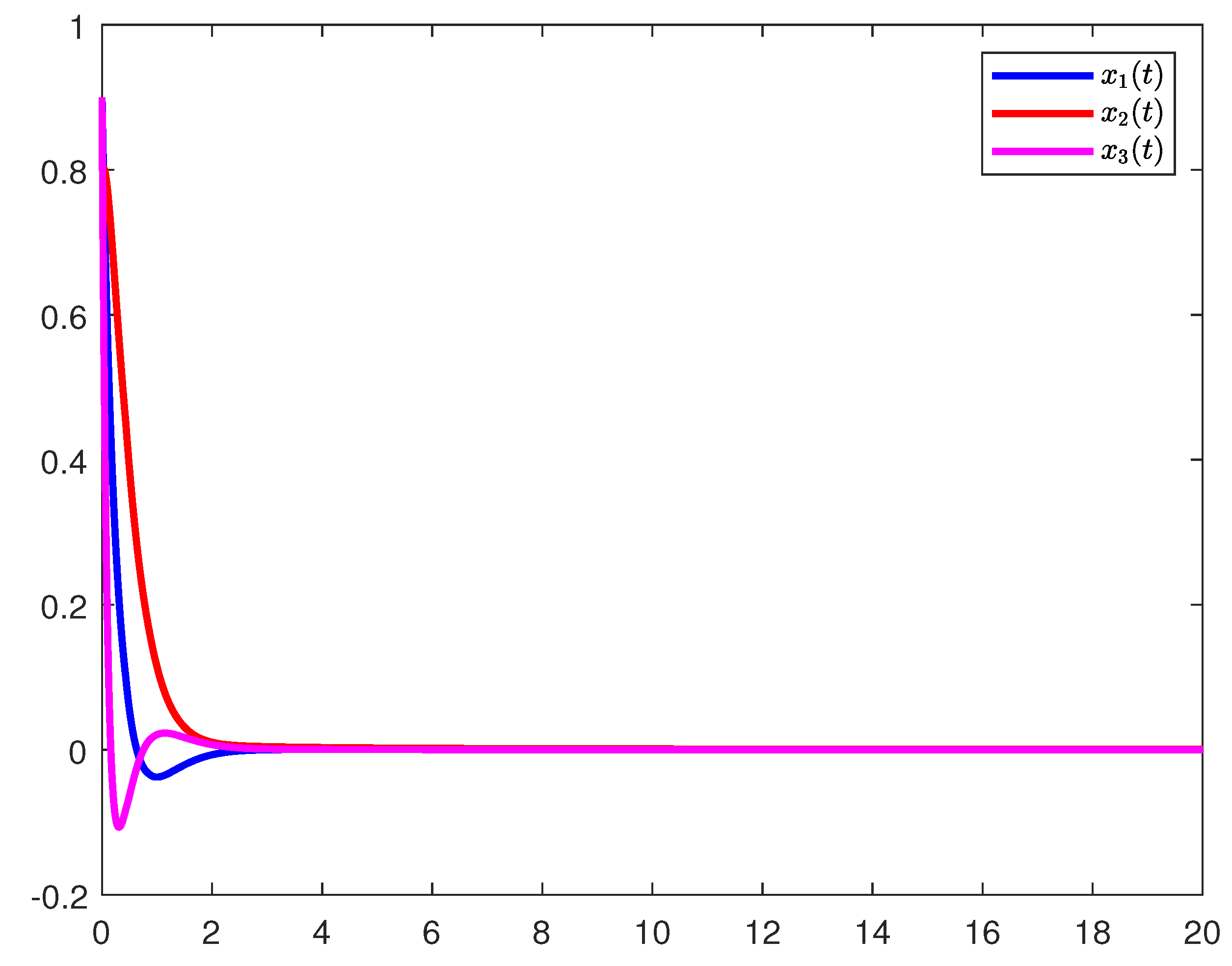
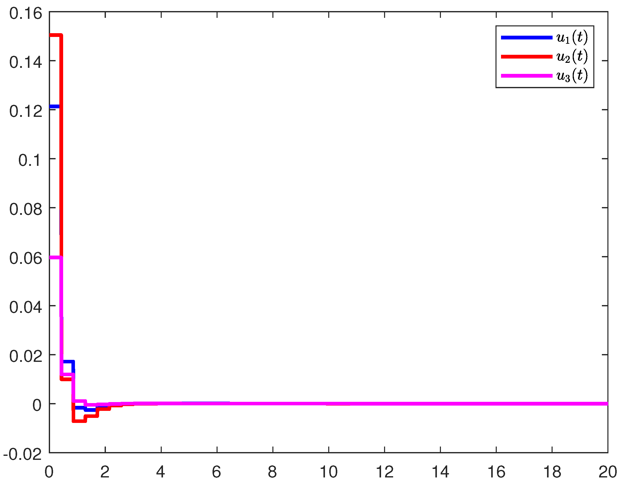
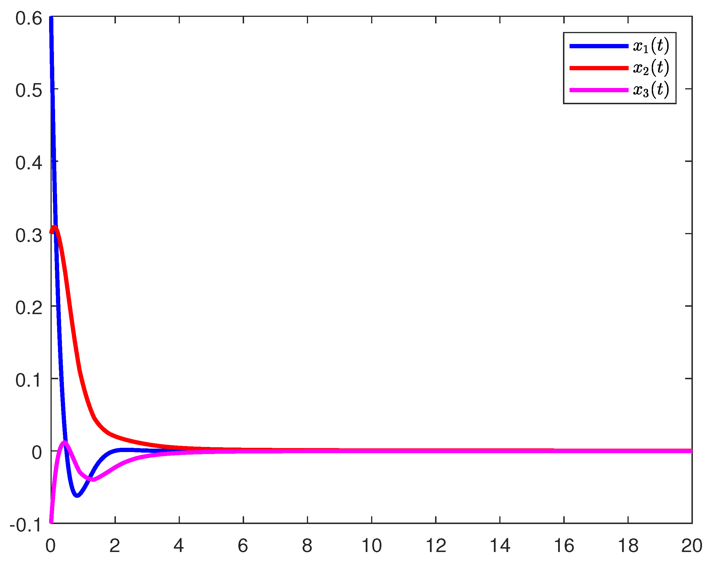
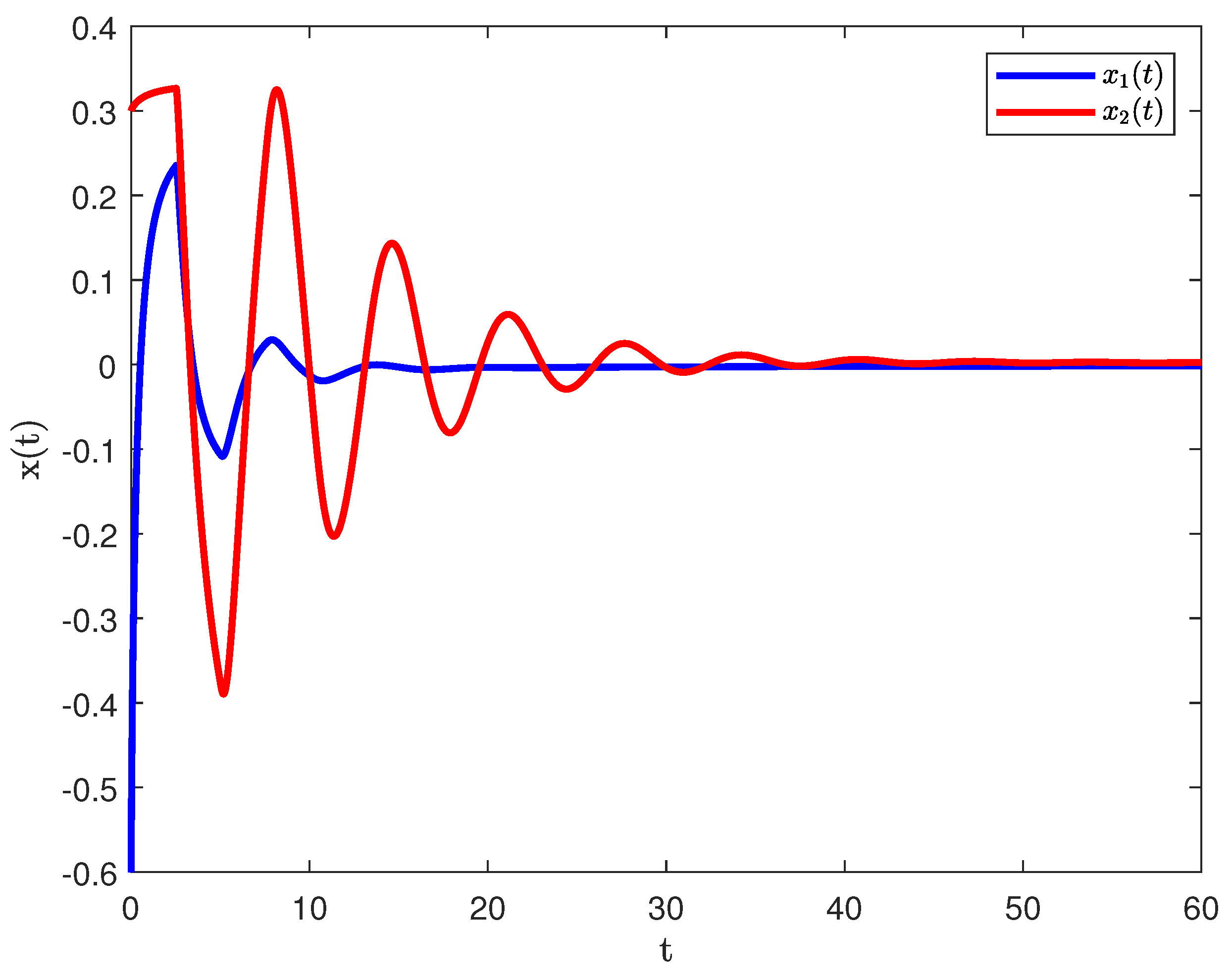
4. Numerical Examples

Three examples are provided in this section to demonstrate the viability of the proposed approach. The following are the parameters:

Example 1.

Consider the model (42) of the following parameters provided in [26]

$$\begin{array}{c}\hfill A=\left[\begin{array}{ccc}-5& 0& 0\\ 0& -4& 0\\ 0& 0& -9\end{array}\right],B=\left[\begin{array}{ccc}2& -1.2& 0\\ 1.8& 1.71& 1.15\\ -4.75& 0& 1.1\end{array}\right],\end{array}$$

and activation functions $f_i(·)=tanh(·)(i=1,2,3)$ with $L=diag(1,1,1)$. The maximum ϖ can be acquired by utilizing the MATLAB LMI toolbox to solve the LMIs of Corollary 2. For different δ, the maximum ϖ calculated by Corollary 2 is shown in

Table 1. The maximum $\varpi$ allowed for different $\delta$ of Example 1.

$\mathit{\delta }$	0.9	0.92	0.95	0.98
[26]	0.13	0.14	0.15	0.17
Corollary 2	0.410	0.415	0.423	0.431

and compared with the results of the previous literature. It is obvious that in comparison the results obtained by the method in this article have a greater improvement advantage. Distinctly, when δ takes $0.9$, $0.92$, $0.95$, and $0.98$, the maximum ϖ is $0.410$, $0.415$, $0.423$, and $0.431$, which is an increase of $215.3\%$, $196.4\%$, $182\%$, and $153.5\%$ compared with [26], respectively. Furthermore, taking $\delta =0.98$, $\varpi =0.4315$, the corresponding controller gain can be obtained as

$$K=\left[\begin{array}{ccc}0.1163& 0.0134& 0.0066\\ 0.1627& -0.0114& 0.0146\\ 0.0484& 0.0163& 0.0034\end{array}\right].$$

For the purpose of obtaining simulation results, the initial value is considered as $\xi \left(t_0\right)={[0.9,0.8,0.9]}^T$, and through the derived matrix K, the curve of state responses for model (42) is exhibited in Figure 1. Figure 2 reflects the sampled-data control input $u\left(t\right)$. It is evident from Figure 1 that the FONNs can reach stability in a short time. The sampled-data controller’s discrete feature is depicted in Figure 2. The obtained results verify the superiority of the proposed approaches in this paper.

Example 2.

Consider the model (42) of the following parameters provided in [22]

$$\begin{array}{c}\hfill A=\left[\begin{array}{ccc}-6& 0& 0\\ 0& -2& 0\\ 0& 0& -2\end{array}\right],B=\left[\begin{array}{ccc}3& -2& -2\\ 1& 1& 0\\ 1& 0& 1\end{array}\right],\end{array}$$

taking the activation functions $f_i(·)=tanh(·)(i=1,2,3)$ with $L=diag(1,1,1)$. For different δ, applying the MATLAB LMI toolbox, the maximum ϖ is obtained by resolving the Equations (50)–(52) in Corollary 2, as displayed in

Table 2. The maximum $\varpi$ allowed for different $\delta$ of Example 2.

$\mathit{\delta }$	0.9	0.92	0.95	0.98
[22]	0.12	0.13	0.15	0.16
Corollary 2	0.426	0.432	0.440	0.448

. As can be observed in Table 2, a less conservative condition for delay-dependent and order-dependent stability can be developed by using the fractional-order Leibniz–Newton formula and creating the suitable LKFs. When δ takes different values of $0.9$, $0.92$, $0.95$, and $0.98$, the maximum ϖ is $0.426$, $0.432$, $0.440$, and $0.448$. The maximum ϖ of the reference [22] is $0.12$, $0.13$, $0.15$, and $0.16$, which is $255\%$, $232.3\%$, $193.3\%$, and $180\%$ larger than the reference [22], respectively. Additionally, choose $\delta =0.98$, $\varpi =0.448$. The controller gain matrix K is designed as

$$K=\left[\begin{array}{ccc}-0.0021& 0.0321& 0.0321\\ 0.0360& -0.3117& -0.1935\\ 0.0360& -0.1935& -0.3117\end{array}\right].$$

Based on the above result, so as to acquire the simulation results, the initial value $\xi \left(t_0\right)={[0.6,0.3,-0.1]}^T$ is selected. Figure 3 shows the model’s state response curve (42). As can be seen from Figure 3, the FONNs can achieve stability for a brief moment. Figure 4 depicts the corresponding control input when ZOH is implemented. As a result, the simulation results presented above attest to the viability and efficiency of the FONNs based on sampled-data control.

Example 3.

Consider the model (54) of the following parameters provided in [33]

$$\begin{array}{c}\hfill A=\left[\begin{array}{cc}-2& 0\\ 0& -0.9\end{array}\right],B=\left[\begin{array}{cc}-1& 0\\ -1& -1\end{array}\right],\end{array}$$

by solving Corollary 3, the maximum delay of the model (54) can be obtained.

Table 3. The maximum delay $\sigma$ allowed for different $\delta$.

$\mathit{\delta }$	0.8	0.85	0.9	0.95	0.98
[33] [ $\dot{\tau }\left(t\right)$ = 0, $u\left(t\right)$ = 0]	N/A	N/A	N/A	N/A	N/A
[20] [Theorem 3.1]	∞	∞	∞	∞	∞
[34] [ $\mu$ = 0, $u\left(t\right)$ = 0]	0.384	0.414	0.443	0.471	0.488
[35]	0.840	0.882	0.925	0.962	0.984
Corollary 3	2.501	2.413	2.341	2.283	2.253

shows the results of different δ corresponding to different maximum delay σ. From Table 3, we can see that in reference [20], although the authors give the stability condition of delay dependence and order dependence for fractional-order time-delay systems, this criterion does not actually depend on delay or order, and it is very conservative (reference [34] gives the corresponding proof). So, through numerical comparison, it can be found that our stable upper bound is larger than that in the previous literature. It can be seen that with the innovative construction of the LKF method and the appropriate introduction of the fractional-order Leibniz–Newton formula, we can obtain a less conservative order-dependent and delay-dependent stability criterion.

According to the solution results, given the initial condition $\psi \left(t\right)={[-0.6,0.3]}^T$, the state trajectory of the model can be simulated, as shown in Figure 5. Therefore, from the comparison table and the state simulation trajectory chart, it can be seen that our results are significantly superior to the existing results.

5. Conclusions

In this paper, the stability of FONNs with time delay in light of sampled-data control has been studied. On the basis of the newly constructed LKFs and the newly proposed fractional-order Leibniz–Newton formula, the sufficient conditions for stable-order dependence and delay dependence have been established. Eventually, the validity of the theoretical results was verified by three numerical simulations. In addition, some of the issues discussed in [36,37,38] (fractional-order chaotic or hyperchaotic systems, synchronous communication of fractional-order chaotic systems, and event-triggered impulsive chaotic synchronization of fractional-order systems) are also interesting and will be further considered in future work.

References

1. Mandelbrot, B.B. The Fractal Geometry of Nature; WH Freeman: New York, NY, USA, 1982. [Google Scholar]
2. Kilbas, A.A.; Marichev, O.I.; Samko, S.G. Fractional Integrals and Derivatives (Theory and Applications); Gordon and Breach: Yverdon, Switzerland, 1983. [Google Scholar]
3. Hilfer, R. Applications of Fractional Calculus in Physics; World Scientific: Singapore, 2000. [Google Scholar]
4. Oppenheim, A.V.; Willsky, A.S.; Nawab, S.H.; Ding, J.J. Signals and Systems; Prentice Hall: Upper Saddle River, NJ, USA, 1997. [Google Scholar]
5. Kilbas, A.A.; Srivastava, H.M.; Trujillo, J.J. Theory and Applications of Fractional Differential Equations; Elsevier: Amsterdam, The Netherlands, 2006. [Google Scholar]
6. Delavari, H.; Mohadeszadeh, M. Robust finite-time synchronization of non-identical fractional-order hyperchaotic systems and its application in secure communication. IEEE/CAA J. Autom. Sin. 2016, 6, 228–235. [Google Scholar] [CrossRef]
7. Yousefpour, A.; Jahanshahi, H.; Munoz-Pacheco, J.M.; Bekiros, S.; Wei, Z.C. A fractional-order hyper-chaotic economic system with transient chaos. Chaos Solitons Fractals 2020, 130, 109400. [Google Scholar] [CrossRef]
8. Zeng, D.Q.; Wu, K.T.; Zhang, R.M.; Zhong, S.; Shi, K.B. Improved results on sampled-data synchronization of Markovian coupled neural networks with mode delays. Neurocomputing 2018, 275, 2845–2854. [Google Scholar] [CrossRef]
9. Zhang, G.L.; Zhang, J.Y.; Li, W.; Ge, C.; Liu, Y.J. Robust synchronization of uncertain delayed neural networks with packet dropout using sampled-data control. Appl. Intell. 2021, 51, 9054–9065. [Google Scholar] [CrossRef]
10. Wang, H.; Ni, Y.J.; Wang, J.W.; Tian, J.P.; Ge, C. Sampled-data control for synchronization of Markovian jumping neural networks with packet dropout. Appl. Intell. 2022, 53, 8898–8909. [Google Scholar] [CrossRef]
11. Picozzi, S.; West, B.J. Fractional Langevin model of memory in financial markets. Phys. Rev. E 2002, 66, 046118. [Google Scholar] [CrossRef] [PubMed]
12. Zhang, W.W.; Cao, J.D.; Chen, D.Y.; Alsaadi, F.E. Synchronization in fractional-order complex-valued delayed neural networks. Entropy 2018, 20, 54. [Google Scholar] [CrossRef]
13. Thuan, M.V.; Binh, T.N.; Huong, D.C. Finite-time guaranteed cost control of Caputo fractional-order neural networks. Asian J. Control 2020, 22, 696–705. [Google Scholar] [CrossRef]
14. Xu, S.; Liu, H.; Han, Z.M. The passivity of uncertain fractional-order neural networks with time-varying delays. Fractal Fract. 2022, 6, 375. [Google Scholar] [CrossRef]
15. Wang, C.X.; Zhou, X.D.; Shi, X.Z.; Jin, Y.T. Delay-dependent and order-dependent LMI-based sliding mode H control for variable fractional order uncertain differential systems with time-varying delay and external disturbance. J. Frankl. Inst. 2022, 359, 7893–7912. [Google Scholar] [CrossRef]
16. Chen, Y.; Wang, B.; Chen, Y.; Wang, Y. Sliding Mode Control for a Class of Nonlinear Fractional Order Systems with a Fractional Fixed-Time Reaching Law. Fractal Fract. 2022, 6, 678. [Google Scholar] [CrossRef]
17. Jia, T.; Chen, X.; He, L.; Zhao, F.; Qiu, J. Finite-Time Synchronization of Uncertain Fractional-Order Delayed Memristive Neural Networks via Adaptive Sliding Mode Control and Its Application. Fractal Fract. 2022, 6, 502. [Google Scholar] [CrossRef]
18. Stamova, I.; Henderson, J. Practical stability analysis of fractional-order impulsive control systems. Isa Trans. 2016, 64, 77–85. [Google Scholar] [CrossRef]
19. Guo, L.; Ali Shah, K.; Bai, S.; Zada, A. On the Analysis of a Neutral Fractional Differential System with Impulses and Delays. Fractal Fract. 2022, 6, 673. [Google Scholar] [CrossRef]
20. Chen, L.P.; Wu, R.C.; Cheng, Y.; Chen, Y.Q. Delay-dependent and order-dependent stability and stabilization of fractional-order linear systems with time-varying delay. IEEE Trans. Circuits Syst. II Express Briefs 2020, 67, 1064–1068. [Google Scholar] [CrossRef]
21. Ma, Z.; Sun, K. Nonlinear Filter-Based Adaptive Output-Feedback Control for Uncertain Fractional-Order Nonlinear Systems with Unknown External Disturbance. Fractal Fract. 2023, 7, 694. [Google Scholar] [CrossRef]
22. Zhang, Q.; Wang, H.; Wang, L. Order-dependent sampling control for state estimation of uncertain fractional-order neural networks system. Optim. Control Appl. Methods, 2023; under review. [Google Scholar]
23. Cao, K.; Gu, J.; Mao, J.; Liu, C. Sampled-Data Stabilization of Fractional Linear System under Arbitrary Sampling Periods. Fractal Fract. 2022, 6, 416. [Google Scholar] [CrossRef]
24. Cao, K.C.; Qian, C.J.; Gu, J.P. Sampled-data control of a class of uncertain nonlinear systems based on direct method. Syst. Control Lett. 2021, 155, 105000. [Google Scholar] [CrossRef]
25. Li, S.; Ahn, C.K.; Guo, J.; Xiang, Z.R. Neural network-based sampled-data control for switched uncertain nonlinear systems. IEEE Trans. Syst. Man Cybern. Syst. 2019, 51, 5437–5445. [Google Scholar] [CrossRef]
26. Zhang, Q.; Ge, C.; Zhang, R.N.; Yang, L. Order-dependent sampling control of uncertain fractional-order neural networks system. Authorea, 2022; Preprints. [Google Scholar]
27. Agarwal, R.P.; Hristova, S.; O’Regan, D. Lyapunov Functions and Stability Properties of Fractional Cohen—GrossbergNeural Networks Models with Delays. Fractal Fract. 2023, 7, 732. [Google Scholar] [CrossRef]
28. Chen, L.; Gong, M.; Zhao, Y.; Liu, X. Finite-Time Synchronization for Stochastic Fractional-Order Memristive BAM Neural Networks with Multiple Delays. Fractal Fract. 2023, 7, 678. [Google Scholar] [CrossRef]
29. Zhao, K. Stability of a Nonlinear Langevin System of ML-Type Fractional Derivative Affected by Time-Varying Delays and Differential Feedback Control. Fractal Fract. 2022, 6, 725. [Google Scholar] [CrossRef]
30. Duarte-Mermoud, M.A.; Aguila-Camacho, N.; Gallegos, J.A.; Castro-Linares, R. Using general quadratic Lyapunov functions to prove Lyapunov uniform stability for fractional order systems. Commun. Nonlinear Sci. Numer. Simul. 2015, 22, 650–659. [Google Scholar] [CrossRef]
31. Jia, J.; Huang, X.; Li, Y.X.; Cao, J.D.; Alsaedi, A. Global stabilization of fractional-order memristor-based neural networks with time delay. IEEE Trans. Neural Netw. Learn. Syst. 2019, 31, 997–1009. [Google Scholar] [CrossRef] [PubMed]
32. Xiong, J.L.; Lam, J. Stabilization of networked control systems with a logic ZOH. IEEE Trans. Autom. Control 2009, 54, 358–363. [Google Scholar] [CrossRef]
33. Hu, T.T.; He, Z.; Zhang, X.J.; Zhong, S.M.; Yao, X.Q. New fractional-order integral inequalities: Application to fractional-order systems with time-varying delay. J. Frankl. Inst. 2021, 358, 3847–3867. [Google Scholar] [CrossRef]
34. Jin, X.C.; Lu, J.G. Order-dependent and delay-dependent conditions for stability and stabilization of fractional-order time-varying delay systems using small gain theorem. Asian J. Control 2023, 25, 1365–1379. [Google Scholar] [CrossRef]
35. Jin, X.C.; Lu, J.G. Order-dependent LMI-based stability and stabilization conditions for fractional-order time-delay systems using small gain theorem. Int. J. Robust Nonlinear Control 2022, 32, 6484–6506. [Google Scholar] [CrossRef]
36. Sene, N.; Ndiaye, A. On Class of Fractional-Order Chaotic or Hyperchaotic Systems in the Context of the Caputo Fractional-Order Derivative. J. Math. 2020, 2020, 8815377. [Google Scholar] [CrossRef]
37. Li, Q.P.; Liu, S.Y.; Chen, Y.G. Combination event-triggered adaptive networked synchronization communication for nonlinear uncertain fractional-order chaotic systems. Appl. Math. Comput. 2018, 333, 521–535. [Google Scholar] [CrossRef]
38. Yu, N.X.; Zhu, W. Event-triggered impulsive chaotic synchronization of fractional-order differential systems. Appl. Math. Comput. 2021, 388, 125554. [Google Scholar] [CrossRef]
Figure 1. State responses for Example 1.
Fractalfract 07 00876 g001
Figure 2. Sampled-data control input for Example 1.
Fractalfract 07 00876 g002
Figure 3. State responses for Example 2.
Fractalfract 07 00876 g003
Figure 4. Sampled-data control input for Example 2.
Fractalfract 07 00876 g004
Figure 5. State responses for Example 3.
Fractalfract 07 00876 g005