The Analytical Solutions to the Fractional Kraenkel–Manna–Merle System in Ferromagnetic Materials

Abstract

In this article, we examine the Kraenkel–Manna–Merle system (KMMS) with an M-truncated derivative (MTD). Our goal is to obtain rational, hyperbolic, and trigonometric solutions by using the $\mathcal{F}$-expansion technique with the Riccati equation. To our knowledge, no one has studied the exact solutions to the KMMS in the presence/absence of a damping effect with an M-truncated derivative, using the $\mathcal{F}$-expansion technique. The magnetic field propagation in a zero-conductivity ferromagnet is described by the KMMS; hence, solutions to this equation may provide light on several fascinating scientific phenomena. We use MATLAB to display figures in a variety of 3D and 2D formats to demonstrate the influence of the M-truncated derivative on the exact solutions to the KMMS.

1. Introduction

The fractional differential equations (FDEs) are used in many disciplines including mathematical biology, physics, quantum field theory, neural physics, solid state physics, fluid mechanics, plasma physics, and optical fibers [1,2,3]. Moreover, the idea of the fractional derivative has been utilized to characterize a broad variety of phenomena in many areas such as a porous medium, fluid dynamics, ocean waves, signal processing, plasma physics, electromagnetism, wave propagation, chaotic systems, photonics, and optical fiber communication.

Due to the tremendous advances in information technology to meet the need for large data and high-density storage, there has been an abundance of interesting studies on ferromagnetic materials over the past several decades. As a result of recent technological advances, tiny ferromagnetic particles may now be fabricated. It is critical to gain a better understanding of the features of micro- and supermicrostructures in nanoscale ferrous metals [4,5,6,7,8]. In the case of such magnetization, tiny nanoparticles could be thought of as homogeneous over these particles and can be represented by a magnetic moment. The dipolar motions of the magnetic moments allow ferromagnetic particles to communicate. Solitons are constantly produced as a result of these interactions. In consequence, a wide variety of solitary waves’ dissemination phenomena has been examined.

The exact solution to the differential equation must be obtained in order to describe whether the soliton is destroyed after the collision. However, solving nonlinear partial differential equations has long been a tough but critical endeavor. As a result, many brilliant scientists in the domains of science and engineering have developed a number of strong approaches for acquiring exact solutions, for instance, improved $tan(\phi /2)$-expansion [9], such as the $(G^{\prime }/G)$-expansion method [10,11], the Kudryashov method [12], the first-integral method [13], the sine–cosine [14,15], the $exp(-\varphi (\varsigma \left)\right)$-expansion [16], the direct algebraic [17], the perturbation method [18,19], the tanh–sech [20,21], the sine-Gordon expansion [22], the Jacobi elliptic function [23], and so on.

In this article, we take into consideration the Kraenkel–Manna–Merle system with an M-truncated derivative (KMMS-MTD):

$$\left\{\begin{array}{c}{\mathfrak{D}}_{i,t}^{\alpha ,\beta }{\Phi }_x-\Phi {\Psi }_x+\kappa {\Psi }_x=0,\hfill \\ {\mathfrak{D}}_{i,t}^{\alpha ,\beta }{\Psi }_x-\Phi {\Phi }_x=0,\hfill \end{array}\right.$$

(1)

where $\Phi =\Phi (x,t)$ represents the magnetization, $\Psi =\Psi (x,t)$ represents the external magnetic fields, and $\kappa$ denotes the damping coefficient. Nguepjouo et al. [24] investigated a combination of magnetization density expansion and coordinate transformations and converted the structure into the following type:

$$\left\{\begin{array}{c}{\Phi }_{xt}-\Phi {\Psi }_x+\kappa {\Psi }_x=0,\hfill \\ {\Psi }_{xt}-\Phi {\Phi }_x=0,\hfill \end{array}\right.$$

(2)

which may describe the nonlinear propagation of short waves in saturated ferromagnetic materials with zero conductivity. When damping is neglected ($\kappa =0$), Equation (2) is integrable and has Lax pairings. Numerous researchers have developed many approaches for acquiring the solutions to the KMMS (2) with $\kappa =0$, including the bilinear method [24], the inverse scattering method [25], the ($G^{\prime }/G$)-expansion method [26], the auxiliary equation method [27], the semi-inverse technique and the new auxiliary equation method [28], the mapping method [29], etc. However, the fractional derivative of the KMMS (2) with an M-truncated derivative has not been treated until now.

The novelty of this paper is to obtain the exact solutions to the KMMS-MTD (1). We use the F-expansion technique in order to obtain the rational, hyperbolic, and trigonometric solutions to (1). We consider two different cases either with damping (i.e., $\kappa \ne 0$) or without damping (i.e., $\kappa =0$). We extend some previous results including the results reported in [28]. The solutions offered here would be very helpful to physicists in understanding important physical phenomena, since the KMMS illustrates how nonlinear short waves travel through ferromagnetic materials with zero conductivity in an external area. In addition, we give a few graphical representations created using MATLAB software to study the effect of the MTD on the acquired solutions to the KMMS-MTD (1). We deduce that the surface moves to the right as the order of derivatives increases.

The article proceeds as follows: In the next section, we define the MTD and list its characteristics. Then, we obtain the wave equation for the KMMS-MTD (1) in Section 3. In Section 4, the F-expansion method is used to provide an exact solution to the KMMS-MTD (1). In Section 5, we discuss the effect of the MTD on the obtained solutions. Finally, the conclusions of the work are presented.

2. M-Truncated Derivative

Several mathematicians have provided several versions of fractional derivatives. The most common are those suggested by Riesz, Riemann–Liouville, Marchaud Grunwald–Letnikov, Erdelyi, Caputo, and Hadamard [30,31,32,33,34]. Traditional derivative formulae, such as the product rule, quotient rule, and chain rule, do not apply to a large number of fractional derivative types. Sousa et al. [35] recently proposed a novel derivative called the M- truncated derivative (MTD) as follows:

Definition 1 

([35,36]). The MTD for the function $\phi :[0,\infty )\to \mathbb{R}$ of order $\alpha \in (0,1]$ is defined as

$${\mathfrak{D}}_{i,t}^{\alpha ,\beta }\phi \left(t\right)=\underset{h\to 0}{lim}\frac{\phi \left(t{\mathcal{E}}_{i,\beta }\left(h{t}^{-\alpha }\right)\right)-\phi \left(t\right)}{h},\mathit{for}t>0,$$

where ${\mathcal{E}}_{i,\beta }$ is defined as

$${\mathcal{E}}_{i,\beta }\left(z\right)=\sum _{k=0}^i\frac{z^k}{\Gamma (\beta k+1)},$$

for $\beta >0$ and $z\in \mathbb{C}$.

The following theorem states the features that the MTD must have.

Theorem 1 

([35,36]). If φ and ψ are differentiable functions and a, $b,$ and $\upsilon$ are real constants, then

(1) 

${\mathfrak{D}}_{i,t}^{\alpha ,\beta }(a\phi +b\psi )=a{\mathfrak{D}}_{i,t}^{\alpha ,\beta }\left(\phi \right)+b{\mathfrak{D}}_{i,t}^{\alpha ,\beta }\left(\psi \right)$;

(2) 

${\mathfrak{D}}_{i,t}^{\alpha ,\beta }\left(t^{\nu }\right)=\frac{\nu }{\Gamma (\beta +1)}{t}^{\nu -\alpha }$;

(3) 

${\mathfrak{D}}_{i,t}^{\alpha ,\beta }\left(\phi \psi \right)=\phi {\mathfrak{D}}_{i,t}^{\alpha ,\beta }\psi +\psi {\mathfrak{D}}_{i,t}^{\alpha ,\beta }\phi$;

(4) 

${\mathfrak{D}}_{i,t}^{\alpha ,\beta }\left(\phi \right)\left(t\right)=\frac{t^{1-\alpha }}{\Gamma (\beta +1)}\frac{d\phi }{dt}$;

(5) 

${\mathfrak{D}}_{i,t}^{\alpha ,\beta }(\phi \circ \psi )\left(t\right)={\phi }^{\prime }\left(\psi \left(t\right)\right){\mathfrak{D}}_{i,t}^{\alpha ,\beta }\psi \left(t\right)$.

3. Traveling Wave Equation for the KMMS-MTD

Using the following wave transformation

$$\Psi (x,t)=\psi \left(\xi \right),\Phi (x,t)=\phi \left(\xi \right)\mathrm{and}\xi ={\xi }_{1}x+\frac{{\xi }_2\Gamma (\beta +1)}{\alpha }{t}^{\alpha },$$

(3)

where the functions $\psi \left(\xi \right)$ and $\phi \left(\xi \right)$ are real, ${\xi }_1,{\xi }_2$ are non-zero constants, and we are able to obtain the wave equation of the KMMS-MTD (1). Inserting Equation (3) into Equation (1), we obtain

$$\left\{\begin{array}{c}{\xi }_1{\xi }_2{\phi }^{″}+\kappa {\xi }_1{\psi }^{\prime }-{\xi }_1\phi {\psi }^{\prime }=0,\hfill \\ {\xi }_1{\xi }_2{\psi }^{″}-{\xi }_1\phi {\phi }^{\prime }=0.\hfill \end{array}\right.$$

(4)

Therefore, Equation (4) becomes

$$\left\{\begin{array}{c}{\xi }_2{\phi }^{″}+\kappa {\psi }^{\prime }-\phi {\psi }^{\prime }=0,\hfill \\ {\xi }_2{\psi }^{″}-\phi {\phi }^{\prime }=0.\hfill \end{array}\right.$$

(5)

Integrating the second equation in (5) once, we have

$${\psi }^{\prime }=\frac{1}{2{\xi }_2}{\phi }^2+\frac{c_0}{{\xi }_2}.$$

(6)

Substituting Equation (6) into first equation in (5), we obtain

$${\phi }^{″}+{\gamma }_3{\phi }^3+{\gamma }_2{\phi }^2+{\gamma }_1\phi +{\gamma }_0=0,$$

(7)

where

$${\gamma }_0=\frac{\kappa c_0}{{\xi }_2^2},{\gamma }_1=\frac{-c_0}{{\xi }_2^2},{\gamma }_2=\frac{\kappa }{2{\xi }_2^2},\mathrm{and}{\gamma }_3=\frac{-1}{2{\xi }_2^2}.$$

4. Exact Solutions to the KMMS-MTD (1)

The solutions to the wave Equation (7) are discovered using the $\mathcal{F}$-expansion method (see, for more details [37]). After that, the exact solutions to the KMMS-MTD (1) can be obtained. Let the solution $\phi$ to Equation (7) be:

$$\phi \left(\xi \right)=a_0+\sum _{k=1}^M(a_k{\mathcal{F}}^k+\frac{b_k}{{\mathcal{F}}^k}),$$

(8)

where $\mathcal{F}$ is the solution of

$${\mathcal{F}}^{\prime }={\mathcal{F}}^2+\varpi .$$

(9)

Equation (9) has the solutions:

$$\mathcal{F}\left(\xi \right)=\sqrt{\varpi }tan\left(\sqrt{\varpi }\xi \right)\mathrm{or}\mathcal{F}\left(\xi \right)=-\sqrt{\varpi }cot\left(\sqrt{\varpi }\xi \right),$$

(10)

if $\varpi >0,$

$$\mathcal{F}\left(\xi \right)=-\sqrt{-\varpi }tanh\left(\sqrt{-\varpi }\xi \right)\mathrm{or}\mathcal{F}\left(\xi \right)=-\sqrt{-\varpi }coth\left(\sqrt{-\varpi }\xi \right),$$

(11)

if $\varpi <0,$ or

$$\phi \left(\xi \right)=\frac{-1}{\xi },$$

(12)

or if $\varpi =0.$

Calculating M requires balancing ${\phi }^{″}$ with ${\phi }^3$ in Equation (7) as follows:

$$M+3=2M\Rightarrow M=1.$$

Equation (8) becomes

$$\phi \left(\xi \right)=a_0+a_1\mathcal{F}+\frac{b_1}{\mathcal{F}}.$$

(13)

Let us examine two separate cases that both rely on $\kappa$(damping term).

4.1. The KMMS-MTD without the Damping Term

Here, we assume that $\kappa =0$; then, Equation (7) takes the form

$${\phi }^{″}+{\gamma }_3{\phi }^3+{\gamma }_1\phi =0.$$

(14)

Setting Equation (13) into Equation (14), we attain

$$\begin{array}{ccc}& & (2a_1+{\gamma }_3{a}_1^3){\mathcal{F}}^3+\left(3a_0{a}_1^2\right){\mathcal{F}}^2+(2\varpi a_1+3{\gamma }_3{a}_0^2{a}_1\hfill \\ & & +3{\gamma }_3{a}_1^2{b}_1+{\gamma }_1{a}_1)\mathcal{F}+({\gamma }_3{a}_0^3+6{\gamma }_3{a}_0{a}_1{b}_1+{\gamma }_1{a}_0)\hfill \\ & & +(2\varpi b_1+3{\gamma }_3{a}_0^2{b}_1+3{\gamma }_3{a}_1{b}_1^2+{\gamma }_1{b}_1){\mathcal{F}}^{-1}+\hfill \\ & & \left(3a_0{a}_1^2\right){\mathcal{F}}^{-2}+(2b_1{\varpi }^2+{\gamma }_3{b}_1^3){\mathcal{F}}^{-3}=0.\hfill \end{array}$$

We compare the coefficients of each power of $\mathcal{F}$ to zero:

$$2a_1+{\gamma }_3{a}_1^3=0,$$

$$3a_0{a}_1^2=0,$$

$$2\varpi a_1+3{\gamma }_3{a}_0^2{a}_1+3{\gamma }_3{a}_1^2{b}_1+{\gamma }_1{a}_1=0,$$

$${\gamma }_3{a}_0^3+6{\gamma }_3{a}_0{a}_1{b}_1+{\gamma }_1{a}_0=0,$$

$$2\varpi b_1+3{\gamma }_3{a}_0^2{b}_1+3{\gamma }_3{a}_1{b}_1^2+{\gamma }_1{b}_1=0,$$

$$3a_0{b}_1^2=0,$$

and

$$2b_1{\varpi }^2+{\gamma }_3{b}_1^3=0.$$

By solving these equations, we obtain the three families of solutions as follows:

First family:

$$a_0=0,a_1=\mp 2\sqrt{\frac{c_0}{2\varpi }},b_1=0,{\xi }_2=\pm \sqrt{\frac{c_0}{2\varpi }}.$$

(15)

Second family:

$$a_0=0,a_1=\mp \sqrt{\frac{-c_0}{\varpi }},b_1=\mp \varpi \sqrt{\frac{-c_0}{\varpi }},{\xi }_2=\pm \sqrt{\frac{-c_0}{4\varpi }}.$$

(16)

Third family:

$$a_0=0,a_1=\mp \sqrt{\frac{c_0}{2\varpi }},b_1=\pm \varpi \sqrt{\frac{c_0}{2\varpi }},{\xi }_2=\pm \sqrt{\frac{c_0}{8\varpi }}.$$

(17)

First family: Equation (14) has the following solution:

$$\phi \left(\xi \right)=\pm 2\sqrt{\frac{c_0}{2\varpi }}\mathcal{F}\left(\xi \right).$$

For $\mathcal{F}\left(\xi \right)$, there are two cases:

Case 1: If $\varpi >0$ and $c_0>0,$ then the solution, with (10) and (3), to the KMMS-MTD (1) is

$${\Phi }_{11}(x,t)=\mp \sqrt{2c_0}tan(\sqrt{\varpi }{\xi }_{1}x\pm \frac{\Gamma (\beta +1)}{\alpha }\sqrt{\frac{c_0}{2}}{t}^{\alpha }),$$

(18)

and

$${\Phi }_{12}(x,t)=\mp \sqrt{2c_0}cot(\sqrt{\varpi }{\xi }_{1}x\pm \frac{\Gamma (\beta +1)}{\alpha }\sqrt{\frac{c_0}{2}}{t}^{\alpha }).$$

(19)

Substituting into Equation (6) and integrating, we obtain

$${\Psi }_{11}(x,t)=\frac{c_0}{{\xi }_2}tan(\sqrt{\varpi }{\xi }_{1}x\pm \frac{\Gamma (\beta +1)}{\alpha }\sqrt{\frac{c_0}{2}}{t}^{\alpha }),$$

(20)

$${\Psi }_{11}(x,t)=\frac{-c_0}{{\xi }_2}cot(\sqrt{\varpi }{\xi }_{1}x\pm \frac{\Gamma (\beta +1)}{\alpha }\sqrt{\frac{c_0}{2}}{t}^{\alpha }).$$

(21)

Case 2: If $\varpi <0$ and $c_0<0,$ then the solution, with (11) and (3), to the KMMS-MTD (1) is

$${\Phi }_{13}(x,t)=\mp \sqrt{-2c_0}tanh(\sqrt{-\varpi }{\xi }_{1}x\pm \frac{\Gamma (\beta +1)}{\alpha }\sqrt{\frac{-c_0}{2}}{t}^{\alpha }),$$

(22)

and

$${\Phi }_{14}(x,t)=\mp \sqrt{-2c_0}coth(\sqrt{-\varpi }{\xi }_{1}x\pm \frac{\Gamma (\beta +1)}{\alpha }\sqrt{\frac{-c_0}{2}}{t}^{\alpha }).$$

(23)

Substituting into Equation (6) and integrating, we obtain

$${\Psi }_{13}(x,t)=\frac{c_0}{{\xi }_2\sqrt{-\varpi }}tanh(\sqrt{-\varpi }{\xi }_{1}x\pm \frac{\Gamma (\beta +1)}{\alpha }\sqrt{\frac{-c_0}{2}}{t}^{\alpha }),$$

(24)

and

$${\Psi }_{14}(x,t)=-\frac{c_0}{{\xi }_2\sqrt{-\varpi }}coth(\sqrt{-\varpi }{\xi }_{1}x\pm \frac{\Gamma (\beta +1)}{\alpha }\sqrt{\frac{-c_0}{2}}{t}^{\alpha }).$$

(25)

Second family: Equation (14) has the solution

$$\phi \left(\xi \right)=\mp \sqrt{\frac{-c_0}{\varpi }}[\mathcal{F}\left(\xi \right)+\varpi {\mathcal{F}}^{-1}\left(\xi \right)].$$

For $\mathcal{F}$$\left(\xi \right)$, there are two cases:

Case 1: If $\varpi >0$ and $c_0<0,$ then the solution, with (10) and (3), to the KMMS-MTD (1) is

$${\Phi }_{15}(x,t)=\pm \sqrt{-c_0}[tan\left(\sqrt{\varpi }\xi \right)+cot\left(\sqrt{\varpi }\xi \right)].$$

(26)

Substituting into Equation (6) and integrating, we obtain

$${\Psi }_{15}(x,t)=\frac{c_0}{{\xi }_2}\xi -\frac{c_0}{2{\xi }_2\sqrt{\varpi }}[tan\left(\sqrt{\varpi }\xi \right)-cot\left(\sqrt{\varpi }\xi \right),$$

(27)

where $\xi ={\xi }_{1}x\pm \frac{\Gamma (\beta +1)}{2\alpha }\sqrt{-\frac{c_0}{\varpi }}{t}^{\alpha }.$

Case 2: If $\varpi <0$ and $c_0>0,$ then the solution, with (11) and (3), to the KMMS-MTD (1) is

$${\Phi }_{16}(x,t)=\mp \sqrt{c_0}[tanh\left(\sqrt{-\varpi }\xi \right)+coth\left(\sqrt{-\varpi }\xi \right)].$$

(28)

Substituting into Equation (6) and integrating, we obtain

$${\Psi }_{16}(x,t)=\frac{c_0}{{\xi }_2}\xi -\frac{c_0}{2{\xi }_2\sqrt{-\varpi }}[tanh\left(\sqrt{-\varpi }\xi \right)+coth\left(\sqrt{-\varpi }\xi \right).$$

(29)

where $\xi ={\xi }_{1}x\pm \frac{\Gamma (\beta +1)}{2\alpha }\sqrt{-\frac{c_0}{\varpi }}{t}^{\alpha }.$

Third family: Equation (14) has the solution

$$\phi \left(\xi \right)=\mp \sqrt{\frac{c_0}{2\varpi }}[\mathcal{F}\left(\xi \right)-\varpi {\mathcal{F}}^{-1}\left(\xi \right)].$$

For $\mathcal{F}\left(\xi \right)$, there are two cases:

Case 1: If $\varpi >0$ and $c_0>0,$ then the solution, with (10) and (3), to the KMMS-MTD (1) is

$${\Phi }_{17}(x,t)=\mp \sqrt{\frac{c_0}{2}}[tan\left(\xi \right)-cot\left(\xi \right)].$$

(30)

Substituting into Equation (6) and integrating, we obtain

$${\Psi }_{17}(x,t)=\frac{c_0}{4\sqrt{\varpi }{\xi }_2}[tan\left(\sqrt{\varpi }\xi \right)-cot\left(\sqrt{\varpi }\xi \right)].$$

(31)

where $\xi ={\xi }_{1}x\pm \frac{\Gamma (\beta +1)}{\alpha }\sqrt{\frac{c_0}{8\varpi }}{t}^{\alpha }.$

Case 2: If $\varpi <0$ and $c_0<0,$ then the solution, with (11) and (3), to the KMMS-MTD (1) is

$${\Phi }_{18}(x,t)=\mp \sqrt{\frac{-c_0}{2}}[tanh\left(\xi \right)-coth\left(\xi \right)].$$

(32)

Substituting into Equation (6) and integrating, we obtain

$${\Psi }_{18}(x,t)=\frac{c_0}{4{\xi }_2}[tanh\left(\sqrt{-\varpi }\xi \right)+coth\left(\sqrt{-\varpi }\xi \right)],$$

(33)

where $\xi ={\xi }_{1}x\pm \frac{\Gamma (\beta +1)}{\alpha }\sqrt{\frac{c_0}{8\varpi }}{t}^{\alpha }.$

Remark 1. 

Putting $\alpha =1$ and $\beta =0$ into Equations (18)–(25), we have the identical solutions to those reported in [28].

4.2. The KMMS-MTD with the Damping Term

We assume now that $\kappa \ne 0;$ then, we put Equation (13) into Equation (7) to obtain:

$$\begin{array}{ccc}& & (2a_1+{\gamma }_3{a}_1^3){\mathcal{F}}^3+(3{\gamma }_3{a}_0{a}_1^2+{\gamma }_2{a}_1^2){\mathcal{F}}^2+(2\varpi a_1+3{\gamma }_3{a}_0^2{a}_1+3{\gamma }_3{a}_1^2{b}_1\hfill \\ & & +{\gamma }_1{a}_1+2{\gamma }_2{a}_0{a}_1)\mathcal{F}+({\gamma }_3{a}_0^3+6{\gamma }_3{a}_0{a}_1{b}_1+{\gamma }_1{a}_0+{\gamma }_0+{\gamma }_2{a}_0^2+2a_1{b}_1)\hfill \\ & & +(2\varpi b_1+3{\gamma }_3{a}_0^2{b}_1+3{\gamma }_3{a}_1{b}_1^2+{\gamma }_1{b}_1+2{\gamma }_2{a}_0{b}_1){\mathcal{F}}^{-1}+\hfill \\ & & (3{\gamma }_3{a}_0{b}_1^2+{\gamma }_2{b}_1^2){\mathcal{F}}^{-2}+(2b_1{\varpi }^2+{\gamma }_3{b}_1^3){\mathcal{F}}^{-3}=0.\hfill \end{array}$$

Equating the coefficients of each power of $\mathcal{F}$ to zero, we obtain a system of algebraic equations. Solving the system, we obtain:

First family:

$$a_0=\frac{\kappa }{3},a_1=\pm 2\sqrt{\frac{c_0}{2\varpi }-\frac{{\kappa }^2}{12\varpi }},b_1=0,\mathrm{and}{\xi }_2=\pm \sqrt{\frac{c_0}{2\varpi }-\frac{{\kappa }^2}{12\varpi }}.$$

Second family:

$$a_0=\frac{\kappa }{3},a_1=\pm \sqrt{\frac{{\kappa }^2}{6\varpi }-\frac{c_0}{\varpi }},b_1=\pm \varpi \sqrt{\frac{{\kappa }^2}{6\varpi }-\frac{c_0}{\varpi }},\mathrm{and}{\xi }_2=\pm \sqrt{\frac{{\kappa }^2}{24\varpi }-\frac{c_0}{4\varpi }}.$$

Third family:

$$a_0=\frac{\kappa }{3},a_1=\pm \sqrt{\frac{c_0}{2\varpi }-\frac{{\kappa }^2}{12\varpi }},b_1=\mp \varpi \sqrt{\frac{c_0}{2\varpi }-\frac{{\kappa }^2}{12\varpi }},\mathrm{and}{\xi }_2=\pm \sqrt{\frac{c_0}{8\varpi }-\frac{{\kappa }^2}{48\varpi }}.$$

First family: Equation (7) has the following solution:

$$\phi \left(\xi \right)=\frac{\kappa }{3}\pm 2\sqrt{\frac{c_0}{2\varpi }-\frac{{\kappa }^2}{12\varpi }}\mathcal{F}\left(\xi \right),\mathrm{for}\frac{c_0}{2\varpi }-\frac{{\kappa }^2}{12\varpi }>0.$$

For $\mathcal{F}\left(\xi \right)$, there are two cases:

Case 1: If $\varpi >0$ and $c_0>\frac{{\kappa }^2}{6},$ then the solution, with (10) and (3), to the KMMS-MTD (1) is

$${\Phi }_{21}(x,t)=\frac{\kappa }{3}\pm 2\sqrt{\frac{c_0}{2}-\frac{{\kappa }^2}{12}}tan\left(\sqrt{\varpi }\xi \right),$$

(34)

and

$${\Phi }_{22}(x,t)=\frac{\kappa }{3}\pm 2\sqrt{\frac{c_0}{2}-\frac{{\kappa }^2}{12}}cot\left(\sqrt{\varpi }\xi \right).$$

(35)

Substituting into Equation (6) and integrating, we obtain

$${\Psi }_{21}(x,t)=\frac{2{\kappa }^2}{9{\xi }_2}\xi \pm \frac{2\kappa }{3}ln|cos(\sqrt{\varpi }\xi )|+2{\xi }_2\sqrt{\varpi }tan\left(\sqrt{\varpi }\xi \right),$$

(36)

and

$${\Psi }_{22}(x,t)=\frac{2{\kappa }^2}{9{\xi }_2}\xi \pm \frac{2\kappa }{3}ln|sin(\sqrt{\varpi }\xi )|-2{\xi }_2\sqrt{\varpi }cot\left(\sqrt{\varpi }\xi \right),$$

(37)

where $\xi ={\xi }_{1}x\pm \frac{\Gamma (\beta +1)}{\alpha }\sqrt{\frac{c_0}{2\varpi }-\frac{{\kappa }^2}{12\varpi }}{t}^{\alpha }.$

Case 2: If $\varpi <0$ and $c_0<\frac{{\kappa }^2}{6},$ then the solution, with (11) and (3), to the KMMS-MTD (1) is

$${\Phi }_{23}(x,t)=\frac{\kappa }{3}\mp 2\sqrt{\frac{{\kappa }^2}{12}-\frac{c_0}{2}}tanh\left(\sqrt{-\varpi }\xi \right),$$

(38)

and

$${\Phi }_{24}(x,t)=\frac{\kappa }{3}\mp 2\sqrt{\frac{{\kappa }^2}{6}-c_0}coth\left(\sqrt{-\varpi }\xi \right).$$

(39)

Substituting into Equation (6) and integrating, we obtain

$${\Psi }_{23}(x,t)=\frac{2{\kappa }^2}{9{\xi }_2}\xi \pm \frac{2\kappa }{3}ln|cosh(\sqrt{-\varpi }\xi )|-2{\xi }_{2}tanh\left(\sqrt{-\varpi }\xi \right),$$

(40)

and

$${\Psi }_{24}(x,t)=\frac{2{\kappa }^2}{9{\xi }_2}\xi \pm \frac{2\kappa }{3}ln|sinh(\sqrt{-\varpi }\xi )|-2{\xi }_2\sqrt{-\varpi }coth\left(\sqrt{-\varpi }\xi \right),$$

(41)

where $\xi ={\xi }_{1}x\pm \frac{\Gamma (\beta +1)}{\alpha }\sqrt{\frac{c_0}{2\varpi }-\frac{{\kappa }^2}{12\varpi }}{t}^{\alpha }.$

Second family: Equation (7) has the solution

$$\phi \left(\xi \right)=\frac{\kappa }{3}\pm \sqrt{\frac{{\kappa }^2}{6\varpi }-\frac{c_0}{\varpi }}[\mathcal{F}\left(\xi \right)+\varpi {\mathcal{F}}^{-1}\left(\xi \right)],\mathrm{for}\frac{{\kappa }^2}{24\varpi }-\frac{c_0}{4\varpi }>0.$$

For $\mathcal{F}$$\left(\xi \right)$, there are two cases:

Case 1: If $\varpi >0$ and $c_0<\frac{{\kappa }^2}{6},$ then the solution, with (10) and (3), to the KMMS-MTD (1) is

$${\Phi }_{25}(x,t)=\frac{\kappa }{3}\pm \sqrt{\frac{{\kappa }^2}{24}-\frac{c_0}{4}}[tan\left(\sqrt{\varpi }\xi \right)+cot\left(\sqrt{\varpi }\xi \right)],$$

(42)

Substituting into Equation (6) and integrating, we obtain

$${\Psi }_{25}(x,t)=(\frac{{\kappa }^2}{18{\xi }_2}+\frac{c_0}{{\xi }_2})\xi \pm \frac{\kappa }{3}ln\left|tan\left(\sqrt{\varpi }\xi \right)\right|+2{\xi }_2\sqrt{\varpi }[tan\left(\sqrt{\varpi }\xi \right)-cot\left(\sqrt{\varpi }\xi \right)],$$

(43)

where $\xi ={\xi }_{1}x\pm \frac{\Gamma (\beta +1)}{\alpha }\sqrt{\frac{{\kappa }^2}{24\varpi }-\frac{c_0}{4\varpi }}{t}^{\alpha }.$

Case 2: If $\varpi <0$ and $c_0>\frac{{\kappa }^2}{6},$ then the solution, with (11) and (3), to the KMMS-MTD (1) is

$${\Phi }_{26}(x,t)=\frac{\kappa }{3}\mp \sqrt{\frac{c_0}{4}-\frac{{\kappa }^2}{24}}[tanh\left(\sqrt{-\varpi }\xi \right)+coth\left(\sqrt{-\varpi }\xi \right)].$$

(44)

Substituting into Equation (6) and integrating, we obtain

$$\begin{array}{ccc}\hfill {\Psi }_{26}(x,t)& =& (\frac{{\kappa }^2}{18{\xi }_2}+\frac{c_0}{{\xi }_2})\xi \pm \frac{\kappa }{3}ln\left|tanh\left(\sqrt{-\varpi }\xi \right)\right|\hfill \\ & & +2{\xi }_2\sqrt{-\varpi }[tanh\left(\sqrt{-\varpi }\xi \right)-coth\left(\sqrt{-\varpi }\xi \right)],\hfill \end{array}$$

(45)

where $\xi ={\xi }_{1}x\pm \frac{\Gamma (\beta +1)}{\alpha }\sqrt{\frac{{\kappa }^2}{24\varpi }-\frac{c_0}{4\varpi }}{t}^{\alpha }.$

Third family: Equation (7) has the solution

$$\phi \left(\xi \right)=\frac{\kappa }{3}\mp \sqrt{\frac{c_0}{2\varpi }-\frac{{\kappa }^2}{12\varpi }}[\mathcal{F}\left(\xi \right)-\varpi {\mathcal{F}}^{-1}\left(\xi \right)],\mathrm{for}\frac{c_0}{2\varpi }-\frac{{\kappa }^2}{12\varpi }>0.$$

For $\mathcal{F}\left(\xi \right)$, there are two cases:

Case 1: If $\varpi >0$ and $c_0>\frac{{\kappa }^2}{6},$ then the solution, with (10) and (3), to the KMMS-MTD (1) is

$${\Phi }_{27}(x,t)=\frac{\kappa }{3}\mp \sqrt{\frac{c_0}{2}-\frac{{\kappa }^2}{12}}[tan\left(\sqrt{\varpi }\xi \right)-cot\left(\sqrt{\varpi }\xi \right)].$$

(46)

Substituting into Equation (6) and integrating, we obtain

$$\begin{array}{ccc}\hfill {\Psi }_{27}(x,t)& =& (\frac{3c_0}{2{\xi }_2}-\frac{{\kappa }^2}{18{\xi }_2})\xi \pm \frac{2\kappa }{3}ln\left|tan\left(\sqrt{\varpi }\xi \right)\right|\hfill \\ & & +2{\xi }_2\sqrt{\varpi }[tan\left(\sqrt{\varpi }\xi \right)+cot\left(\sqrt{\varpi }\xi \right)],\hfill \end{array}$$

(47)

where $\xi ={\xi }_{1}x\pm \frac{\Gamma (\beta +1)}{\alpha }\sqrt{\frac{c_0}{\varpi 8}-\frac{{\kappa }^2}{48\varpi }}{t}^{\alpha }.$

Case 2: If $\varpi <0$ and $c_0<\frac{{\kappa }^2}{6},$ then the solution, with (11) and (3), to the KMMS-MTD (1) is

$${\Phi }_{28}(x,t)=\frac{\kappa }{3}\mp \sqrt{\frac{{\kappa }^2}{12}-\frac{c_0}{2}}[tanh\left(\sqrt{-\varpi }\xi \right)-coth\left(\sqrt{-\varpi }\xi \right)].$$

(48)

Substituting into Equation (6) and integrating, we obtain

$$\begin{array}{ccc}\hfill {\Psi }_{28}(x,t)& =& (\frac{3c_0}{2{\xi }_2}-\frac{{\kappa }^2}{18{\xi }_2})\xi \pm \frac{2\kappa }{3}ln\left|tanh\left(\sqrt{-\varpi }\xi \right)\right|\hfill \\ & & +2{\xi }_2\sqrt{-\varpi }[tanh\left(\sqrt{-\varpi }\xi \right)+coth\left(\sqrt{-\varpi }\xi \right)],\hfill \end{array}$$

(49)

where $\xi ={\xi }_{1}x\pm \frac{\Gamma (\beta +1)}{\alpha }\sqrt{\frac{c_0}{\varpi 8}-\frac{{\kappa }^2}{48\varpi }}{t}^{\alpha }.$

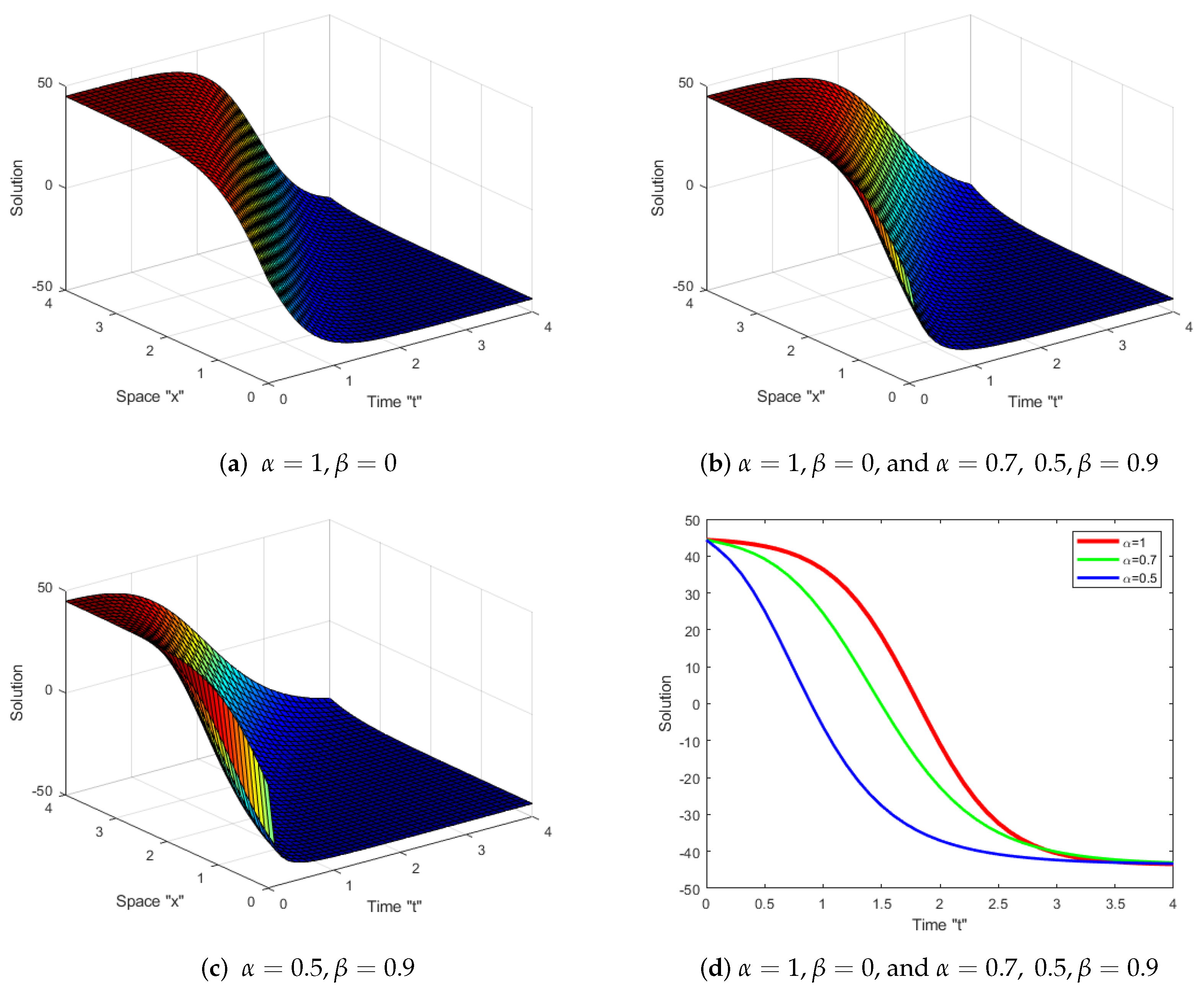
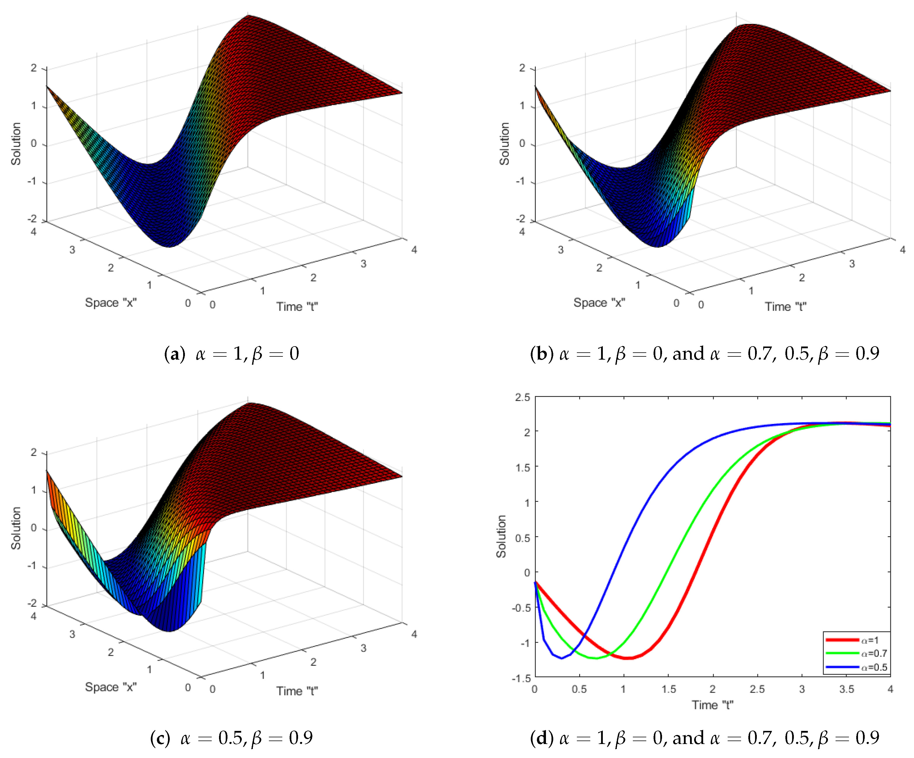
5. Discussion and Graphical Representation

In this paper, we applied the $\mathcal{F}$-expansion method to acquire new rational, hyperbolic, and trigonometric solutions for the Kraenkel–Manna–Merle system. We obtained these exact solutions to the KMMS in the presence and absence of damping terms. Different kinds of solutions with fractional derivatives such as dark soliton, singular solition, periodic solutions, and kink soliton were provided. We investigated how the wave profile was changed for different values of the derivatives order. To understand the nature and behavior of the solutions, it is better to provide graphical illustrations. We provide 2D and 3D figures for the numerous solutions given by (38) and (40). Firstly, we present graphs for the solution to Equation (38). We plotted them when $\varpi =-1$, ${\xi }_1=1$,$x\in [0,4]$, $t\in [0,4],$ and $c_0=-8,$ as follows

Secondly, we give profile of solution of Equation (22). We plotted them with $\varpi =-1$, ${\xi }_1=1$,$x\in [0,4]$, $t\in [0,4],$ and $c_0=-8$, as follows.

From Figure 1 and Figure 2, we can see that the solution curves did not overlap each other. Moreover, as the order of the derivatives rose, the surface moved to the right.

6. Conclusions

In this study, we examined the Kraenkel–Manna–Merle system with an M-truncated derivative (KMMS-MTD) (1), which is used in ferromagnetic materials. We acquired the exact solutions for the KMMS-MTD with and without damping terms by using the $\mathcal{F}$-expansion approach. This approach is efficient and applicable to several initial and boundary value problems. We extended some previous results, such as those stated in [28]. Since Equation (1) is so important for describing magnetic field propagation in a ferromagnet with zero conductivity, the obtained solutions are critical in comprehending a broad variety of fascinating and difficult physical phenomena. Moreover, the MATLAB package was used to show the impact of the M-truncated derivative on the exact solution to the KMMS-MTD (1). We deduced that as the order of the derivatives rose, the surface moved to the right. In future work, we can consider Equation (1) with a stochastic term.

References

1. Yuste, S.B.; Acedo, L.; Lindenberg, K. Reaction front in an A + BC reaction–subdiffusion process. Phys. Rev. E 2004, 69, 036126. [Google Scholar] [CrossRef] [PubMed] [Green Version]
2. Benson, D.A.; Wheatcraft, S.W.; Meerschaert, M.M. The fractional-order governing equation of Lévy motion. Water Resour. Res. 2000, 36, 1413–1423. [Google Scholar] [CrossRef] [Green Version]
3. Iqbal, N.; Wu, R.; Mohammed, W.W. Pattern formation induced by fractional cross-diffusion in a 3-species food chain model with harvesting. Math. Comput. Simul. 2021, 188, 102–119. [Google Scholar] [CrossRef]
4. Newman, N.; Wu, S.Y.; Liu, H.X.; Medvedeva, J.E.; Gu, L.; Singh, R.K.; Yu, Z.G.; Krainsky, I.L.; Krishnamurthy, S.; Smith, D.J.; et al. Recent progress towards the development of ferromagnetic nitride semiconductors for spintronic applications. Phys. Status Solidi A 2006, 203, 2729–2737. [Google Scholar] [CrossRef]
5. Zabel, H. Progress in spintronics. Superlatt Microstruct 2009, 46, 541–553. [Google Scholar] [CrossRef]
6. Shen, B.G.; Sun, J.R.; Hu, F.X.; Zhang, H.W.; Cheng, Z.H. Recent progress in exploring magnetocaloric materials. Adv. Mater. 2009, 21, 4545–4564. [Google Scholar] [CrossRef] [Green Version]
7. Tanaka, M.; Ohya, S.; Hai, P.N. Recent progress in III–V based ferromagnetic semiconductors: Band structure, Fermi level, and tunneling transport. Appl. Phys. Rev. 2014, 1, 011102. [Google Scholar] [CrossRef] [Green Version]
8. Dietl, T.; Sato, K.; Fukushima, T.; Bonanni, A.; Jamet, M.; Barski, A.; Kuroda, S.; Tanaka, M.; Hai, P.N.; Katayama-Yoshida, H. Spinodal nanodecomposition in semiconductors doped with transition metals. Rev. Mod. Phys. 2015, 87, 1311–1377. [Google Scholar] [CrossRef] [Green Version]
9. Manafian, J. Optical soliton solutions for Schrodinger type nonlinear evolution equations by the tan(φ/2)-expansion method. Optik 2016, 127, 4222–4245. [Google Scholar] [CrossRef]
10. Wang, M.L.; Li, X.Z.; Zhang, J.L. The (G/G)-expansion method and travelling wave solutions of nonlinear evolution equations in mathematical physics. Phys. Lett. A 2008, 372, 417–423. [Google Scholar] [CrossRef]
11. Zhang, H. New application of the (G/G)-expansion method. Commun. Nonlinear Sci. Numer. Simul. 2009, 14, 3220–3225. [Google Scholar] [CrossRef]
12. Zafar, A.; Ali, K.K.; Raheel, M.; Jafar, N.; Nisar, K.S. Soliton solutions to the DNA Peyrard-Bishop equation with beta-derivative via three distinctive approaches. Eur. Phys. J. Plus 2020, 135, 1–17. [Google Scholar] [CrossRef]
13. Ewees, A.A.; Abd Elaziz, M.; Al-Qaness, M.A.A.; Khalil, H.A.; Kim, S. Improved Artificial Bee Colony Using Sine-Cosine Algorithm for Multi-Level Thresholding Image Segmentation. IEEE Access 2020, 8, 26304–26315. [Google Scholar] [CrossRef]
14. Wazwaz, A.M. A sine-cosine method for handling nonlinear wave equations. Math. Comput. Model. 2004, 40, 499–508. [Google Scholar] [CrossRef]
15. Yan, C. A simple transformation for nonlinear waves. Phys. Lett. A 1996, 224, 77–84. [Google Scholar] [CrossRef]
16. Khan, K.; Akbar, M.A. The exp(-(ς))-expansion method for finding travelling wave solutions of Vakhnenko-Parkes equation. Int. J. Dyn. Syst. Differ. Equ. 2014, 5, 72–83. [Google Scholar]
17. Sadat, R.; Kassem, M.M. Lie Analysis and Novel Analytical Solutions for the Time-Fractional Coupled Whitham–Broer–Kaup Equations. Int. J. Appl. Comput. Math. 2019, 5, 28. [Google Scholar] [CrossRef]
18. Mohammed, W.W.; Iqbal, N. Impact of the same degenerate additive noise on a coupled system of fractional space diffusion equations. Fractals 2022, 30, 2240033. [Google Scholar] [CrossRef]
19. Mohammed, W.W. Stochastic amplitude equation for the stochastic generalized Swift–Hohenberg equation. J. Egypt. Math. Soc. 2015, 23, 482–489. [Google Scholar] [CrossRef] [Green Version]
20. Wazwaz, A.M. The tanh method: Exact solutions of the Sine–Gordon and Sinh–Gordon equations. Appl. Math. Comput. 2005, 167, 1196–1210. [Google Scholar] [CrossRef]
21. Malfliet, W.; Hereman, W. The tanh method. I. Exact solutions of nonlinear evolution and wave equations. Phys. Scr. 1996, 54, 563–568. [Google Scholar] [CrossRef]
22. Arafa, A.; Elmahdy, G. Application of residual power series method to fractional coupled physical equations arising in fluids flow. Int. J. Differ. Equ. 2018, 2018, 7692849. [Google Scholar] [CrossRef]
23. Yan, Z.L. Abunbant families of Jacobi elliptic function solutions of the dimensional integrable Davey-Stewartson-type equation via a new method. Chaos Solitons Fractals 2003, 18, 299–309. [Google Scholar] [CrossRef]
24. Nguepjouo, F.T.; Kuetche, V.K.; Kofane, T.C. Soliton interactions between multivalued localized waveguide channels within ferrites. Phys. Rev. E 2014, 89, 063201. [Google Scholar] [CrossRef]
25. Tchokouansi, H.T.; Kuetche, V.K.; Kofane, T.C. On the propagation of solitons in ferrites: The inverse scattering approach. Chaos Solitons Fractals 2016, 86, 64–74. [Google Scholar] [CrossRef]
26. Li, B.Q.; Ma, Y.L. Rich soliton structures for the Kraenkel–Manna–Merle (KMM) system in ferromagnetic materials. J. Supercond. Nov. Magn. 2018, 31, 773–1778. [Google Scholar] [CrossRef]
27. Li, B.Q.; Ma, Y.L. Loop-like periodic waves and solitons to the Kraenkel–Manna–Merle system in ferrites. J. Electromagnet. Waves Appl. 2018, 32, 1275–1286. [Google Scholar] [CrossRef]
28. Raza, N.; Hassan, Z.; Butt, A.R.; Rahman, R.U.; Abdel-Aty, A.; Mahmoud, M. New and more dual-mode solitary wave solutions for the Kraenkel–Manna–Merle system incorporating fractal effects. Math. Methods Appl. Sci. 2022, 45, 2964–2983. [Google Scholar] [CrossRef]
29. Mohammed, W.W.; El-Morshedy, M.; Cesarano, C.; Al-Askar, F.M. Soliton Solutions of Fractional Stochastic Kraenkel–Manna–Merle Equations in Ferromagnetic Materials. Fractal Fract. 2023, 7, 328. [Google Scholar] [CrossRef]
30. Katugampola, U.N. New approach to a generalized fractional integral. Appl. Math. Comput. 2011, 218, 860–865. [Google Scholar] [CrossRef] [Green Version]
31. Katugampola, U.N. New approach to generalized fractional derivatives. Bull. Math. Anal. Appl. 2014, 6, 1–15. [Google Scholar]
32. Mouy, M.; Boulares, H.; Alshammari, S.; Alshammari, M.; Laskri, Y.; Mohammed, W.W. On Averaging Principle for Caputo–Hadamard Fractional Stochastic Differential Pantograph Equation. Fractal. Fract. 2023, 7, 31. [Google Scholar] [CrossRef]
33. Kilbas, A.A.; Srivastava, H.M.; Trujillo, J.J. Theory and Applications of Fractional Differential Equations; Elsevier: Amsterdam, The Netherlands, 2016. [Google Scholar]
34. Samko, S.G.; Kilbas, A.A.; Marichev, O.I. Fractional Integrals and Derivatives, Theory and Applications; Gordon and Breach: Yverdon, Switzerland, 1993. [Google Scholar]
35. Sousa, J.V.; de Oliveira, E.C. A new truncated Mfractional derivative type unifying some fractional derivative types with classical properties. Int. J. Anal. Appl. 2018, 16, 83–96. [Google Scholar]
36. Hussain, A.; Jhangeer, A.; Abbas, N.; Khan, I.; Sherif, E.M. Optical solitons of fractional complex Ginzburg–Landau equation with conformable, beta, and M-truncated derivatives: A comparative study. Adv. Differ. Equ. 2020, 2020, 612. [Google Scholar] [CrossRef]
37. Zahrana, E.H.M.; Khater, M.M.A. Modified extended tanh-function method and its applications to the Bogoyavlenskii equation. Appl. Math. Model. 2016, 3, 1769–1775. [Google Scholar] [CrossRef]
Figure 1. (ac) identify the 3D profile of Equation (38), (d) denotes the 2D plot for various values of α at x = 1 , and each solution curve is completely distinct from every other one.
Fractalfract 07 00523 g001
Figure 2. (ac) identify the 3D profile of Equation (40) (d) denotes the 2D plot for various values of α at x = 1 , and each solution curve is completely distinct from every other one.
Fractalfract 07 00523 g002
Disclaimer/Publisher’s Note: The statements, opinions and data contained in all publications are solely those of the individual author(s) and contributor(s) and not of MDPI and/or the editor(s). MDPI and/or the editor(s) disclaim responsibility for any injury to people or property resulting from any ideas, methods, instructions or products referred to in the content.