
Anomalous Thermally Induced Deformation in Kelvin–Voigt Plate with Ultrafast Double-Strip Surface Heating


1
Department of Mathematics, Faculty of Education, Alexandria University, Souter St. El-Shatby, Alexandria P.O. Box 21526, Egypt
2
Mathematics Department, Al-Qunfudhah University College, Umm Al-Qura University, Al-Qunfudhah 28821, Mecca, Saudi Arabia
*
Author to whom correspondence should be addressed.
Fractal Fract. 2023, 7(7), 563; https://doi.org/10.3390/fractalfract7070563
Submission received: 14 June 2023
/
Revised: 12 July 2023
/
Accepted: 17 July 2023
/
Published: 22 July 2023
(This article belongs to the Special Issue Advances in Fractional Order Derivatives and Their Applications)
Abstract
:The Jeffreys-type heat conduction equation with flux precedence describes the temperature of diffusive hot electrons during the electron–phonon interaction process in metals. In this paper, the deformation resulting from ultrafast surface heating on a “nanoscale” plate is considered. The focus is on the anomalous heat transfer mechanisms that result from anomalous diffusion of hot electrons and are characterized by retarded thermal conduction, accelerated thermal conduction, or transition from super-thermal conductivity in the short-time response to sub-thermal conductivity in the long-time response and described by the fractional Jeffreys equation with three fractional parameters. The recent double-strip problem, Awad et al., Eur. Phy. J. Plus 2022, allowing the overlap between two propagating thermal waves, is generalized from the semi-infinite heat conductor case to thermoelastic case in the finite domain. The elastic response in the material is not simultaneous (i.e., not Hookean), rather it is assumed to be of the Kelvin–Voigt type, i.e., , where refers to the stress, is the strain, is the Young modulus, and refers to the strain relaxation time. The delayed strain response of the Kelvin–Voigt model eliminates the discontinuity of stresses, a hallmark of the Hookean solid. The immobilization of thermal conduction described by the ordinary Jeffreys equation of heat conduction is salient in metals when the heat flux precedence is considered. The absence of the finite speed thermal waves in the Kelvin–Voigt model results in a smooth stress surface during the heating process. The temperature contours and the displacement vector chart show that the anomalous heat transfer characterized by retardation or crossover from super- to sub-thermal conduction may disrupt the ultrafast laser heating of metals.
1. Introduction
In many physical situations, thermal conduction may encounter anomalous behavior deviating from the classical diffusive “Fourier” behavior, e.g., heat transfer in fractals, heterogeneous materials, metals with distributed impurities, and nanoscale materials [1,2,3,4,5,6]. Fractional kinetic equations are effective mathematical tools for modeling such anomalous behaviors [7,8,9,10,11,12,13,14,15,16,17,18,19]. A recent fractional version of the Jeffreys equation has been proposed in [20], and under certain circumstances, it can be connected to the continuous-time random walk scheme [21]. The fractional Jeffreys equation with three fractional parameters is a versatile mathematical tool describing many anomalous heat/mass transition behaviors, e.g., acceleration, retardation, and crossover from super- to subdiffusion.
The stresses generated in elastic materials due to thermal effects may cause the material to reach the yield point. Before the yield point, the linearized thermal stress theories with different heat conduction models [6,22,23,24] present successful initial engineering assessments for predicting the stresses and deformations in different types of thermal loadings and heat conductors. One of the earliest studies which presented a prediction of stress distribution induced by anomalous heat/mass transfer is the study of Povstenko [25]; see also the comprehensive monograph by the same author [26]. In [27,28,29,30], different forms of anomalous heat conduction models are adopted and the corresponding thermal stresses are computed. The main feature in most well known fractional heat conduction models is the disappearance of the finite thermal wave speed, with some exceptions to the Atangana–Baleanu fractional derivative [31,32].
The Kelvin–Voigt model is a crucial tool for defining and studying the viscoelastic behavior of certain solid materials in which there is a retardation time in the material response [33]. It differs from the Hookean solid in the retarded response of strain to an applied stress, namely, , where is the retardation time, or the strain relaxation time [34]. When , the Hookean response is recovered, i.e., . The Kelvin–Voigt thermoelasticity has been considered in a variety of viscoelastic applications, e.g., unbounded thermoviscoelastic domain with spherical cavity [35], vibration of an Euler Bernoulli beam [36,37], and micropolar thermoelasticity [38], and has been extended to the second-gradient media [39].
In order to generalize the Danilovskaya problem in hyperbolic thermoelasticity [40,41] to the finite domains, El-Maghraby [42] solved the Lord–Shulman equations for a thick plate with an internal heat source, and the same author [43] solved the Green–Lindsay equations for a thick plate with body force. A similar setting of the thick plate problem in thermoelasticity has been solved for a transversely isotropic medium [44] and has been considered in Kelvin–Voigt medium when a specific form of the fractional dual-phase lag is considered [45]. For ultrafast thermal heating of metals, the deformation resulting from the electronic conduction was considered in [46] for a one-dimension metal film. The authors considered in their formulation that the driving force describes the effect of free carriers on the lattice [47], mathematically described by the term , where is the electron temperature. In the linearized version, the nonlinear term is neglected; thus, the coupling factor is lost. A generalized version of ultrafast thermoelasticity was considered in [48], where the stress includes the lattice temperature and the lattice conduction equation is inserted. If the lattice conduction is neglected and the force describing the effect of free carriers on the lattice is neglected, the resulting ultrafast thermoelasticity corresponds to the dual-phase-lag thermoelasticity with flux precedence [6]; see also [49].
In the present article, we consider a Kelvin–Voigt nanoscale two-dimensional plate with infinite extension subject to an ultrafast surface heating on its upper surface taking the double-strip shape [50,51]. The delayed strain response underlying the Kelvin–Voigt assumption, the nanoscale thickness of the plate, and the ultrafast heating method can be considered as reasoning causes for adopting non-Fourier heat transfer mechanisms such as accelerating, retarding, and crossover from super- to sub-thermal conduction. The Laplace–Fourier transform technique is used to obtain exact solutions in the transformed domain. Then, double infinite summations are numerically implemented to obtain the solutions in the physical domain. The relation between the heat flux and the temperature gradient is shown graphically in different critical instants. We organize the paper as follows: In Section 2, we present the governing equations for the Kelvin–Voigt thermoelasticity with the fractional Jeffreys equation with three fractional parameters. The two-dimensional formulation of the Kelvin–Voigt thermoelastic plate problem is given in Section 3. In Section 4, we derive exact solutions for the temperature, hydrostatic stress, and displacement components in the transformed domain. A suitable numerical technique is adopted in Section 5 to obtain the solution to the physical domain numerically. Lastly, we summarize the work findings in Section 6.
2. Mathematical Model
The governing equations for a homogeneous isotropic thermoviscoelastic material of Kelvin–Voigt type [23,33,34] in the context of the fractional Jeffreys heat conduction equation [20,21] consist of the following:
- (i)
- Stress–strain constitutive relation
- (ii)
- The strain–displacement relation
- (iii)
- Conservation of momentum
Substituting Equation (1) into Equation (3), and using the relations and , we obtain
where and .
- (iv)
- The balance equation for the entropy
Starting from the assumption that for a thermally conducting Kelvin–Voigt solid subject to small strain and small temperature changes [23,38], we have
where is the specific heat at constant strain.
Hence, the energy balance equation is given from (5) and (6) as
The above equations are supplemented with the fractional Jeffery’s heat conduction equation [20,21], namely,
where and are the heat flux and the temperature gradient phase lags [6], respectively, is the thermal conductivity, and . The assumption is adopted to keep the dimension in order [7,52]. The fractional derivative in (8) is defined in the Riemann–Liouville sense [53]:
Substituting Equation (8) into Equation (7), we obtain the energy equation:
3. Problem Formulation
We consider a plate made of a homogeneous isotropic solid occupying the region defined by . The -axis is taken perpendicular to the plate plane and pointing inwards, such that refers to the upper surface and refers to the lower surface. The body is assumed to be initially quiescent. Furthermore, we assume that there are no body forces or heat sources. The upper surface of the plate is assumed to be traction-free and subjected to ultrafast double-strip heating [50], which decays exponentially with time, while the lower surface is assumed to be traction-free and thermally insulated; see Figure 1.
From the above settings, all the considered functions should depend on and . Also, the displacement vector is given in the form
Hence, the governing equations for Kelvin–Voigt thermoelastic plate on the domain consist of the following:
- (i)
- The non-vanishing components of the stress tensor
- (ii)
- The non-vanishing components of the strain tensor
Also, the cubical dilation is given by
- (iii)
- The equations of motion in the absence of body forces along the x- and y-directions, respectively,
By differentiating Equations (19) and (20) with respect to and , respectively, adding the resulting equations and utilizing Equation (18), we obtain
where is the Laplace operator in Cartesian coordinates.
- (i)
- The heat conduction equation in the absence of a heat source
Additionally, it is assumed that the system initiates the experiment in a state of rest with no accelerations, namely,
The governing equations can be put in a more convenient form by using the following non-dimensional variables:
where and .
Using the above non-dimensional variables, Equations (11)–(14), (21), and (22) take the following forms (the asterisks were omitted to avoid confusion):
where and .
We shall consider the hydrostatic stress as the mean value of the normal stresses , and , namely,
By using Equations (28)–(30), we obtain
associated with the following non-dimensional thermal and mechanical boundary conditions
and non-dimensional homogeneous initial conditions
4. Solutions in the Integral-Transform Domain
We shall now define the Laplace transform (denoted by a bar) with respect to a function by the relation [54]
where is a continuous function over time, is the Laplace parameter, and the inverse Laplace’s transform is defined as
where and the Fourier exponential transform (denoted by a hat) to a function with respect to the variable is defined by the relation
with its corresponding inversion
We assume that all the relevant functions are sufficiently smooth on the real line such that the Fourier transform of these functions exists. According to the homogeneous initial conditions (39), upon applying the Laplace transform on both sides of Equations (32) and (33), we arrive at
where
Eliminating between Equations (44) and (45), we obtain
which can be factorized as
where are the roots with positive real parts of the characteristic equation
Upon applying the exponential Fourier transform on Equation (48), we obtain
where , , and . The general solution of Equation (50), bounded for the region , is given as
where , , are parameters depending on and . Similarly, eliminating between Equations (44) and (45) leads to the characteristic equation
Therefore, the general solution of (52) for can be written as
where , , are parameters depending on and . In view of Equations (51), (53) and (45), one can deduce the following relations for and
Using the above relations in Equation (53), we obtain
On the other hand, Equations (17) and (19) can be written in the non-dimensional form as
Taking the Laplace–Fourier transforms for Equations (56) and (57), we obtain
where .
Next, substituting Equations (51) and (55) into the right-hand side of Equation (59), we obtain
where and , , are parameters depending on and .
To determine the tangential component of the velocity, utilizing Equations (51) and (60) in the right-hand side of Equation (58), we obtain
Finally, we combine Equations (51), (55), (60) and (61) with the Laplace and Fourier transforms of Equations (28), (31) and (35), and perform some straightforward calculations; the results are
where
The boundary conditions (36)–(38) in the Laplace–Fourier domain read
Without loss of generality, we specify the condition of double-strip heating [50,51]:
where is the Heaviside unit step function, and is a temporal parameter characterizing the thermalization time, or alternatively, the heating rate. In other words, if we take a dimensional thermalization parameter femtosecond, then at the physical time picosecond, the surface reaches zero temperature difference , or alternatively, the absolute surface temperature becomes identical with the room temperature, . The double-strip heating parameters and are taken as nonzero constants such that (). The boundary surface temperature in the Laplace–Fourier domain is determined by
Equations (67)–(69) immediately give the following system of six linear equations in the unknown parameters and .
This completes the solution of the problem in the Laplace–Fourier-transformed domain.
5. Numerical Results and Discussion
In order to present numerical results, copper material [6,55,56] is chosen for the purposes of numerical evaluation, with the parameters in SI units listed in Table 1.
In addition, we choose the dimensionless plate thickness and the double-strip parameters as
According to the choice of the dimensionless thickness, , and the dimensionless thermalization parameter, , the real thickness of the plate is and the real thermalization parameter equals ; refer to Equation (27), and also see [57].
In this section, we implement two infinite series to calculate the integrals (41) and (43). Thereby, we will bring the temperature, displacement, and hydrostatic stress to the physical domain. Inversion of the Laplace parameter to the physical time requires the implementation of Durbin formula, which is the approximation of the integral (41); see [58,59].
where and is chosen so that . For accelerating the computations time, we use a FORTRAN subroutine [60] for the series with . Inversion of the Fourier transform, i.e., transforming into , requires implementing another integral (refer to (43)), which can be approximated by the following Riemann sum
Using a suitable numerical approach, such as a trapezoidal approach, or a nested approach using the Bulirsch–Stoer step method, the rational function extrapolation, and modified midpoint method [61], the series (80) can be implemented. The parameter takes a value from 100 to 500. The computation time for 100 points ranges from 30 to 180 s depending on the mathematical model, the numerical technique used for inverting the Fourier transform, and the Intel Core processor version. Because of the evanescence of discontinuities in the stresses of the Kelvin–Voigt model and in the temperature of the fractional Jeffreys equation, the running time of the program is much less than that for the elastic case with finite thermal wave speed [57]. The computation was carried out on two Intel Core processors, Core i5-9600K and Core i7-1165G7. MATLAB R2019a was utilized for graphical representations on an NVIDIA Geforce MX330 graphics card.
The heat flux is an important physical vector quantity predicting the actual heat direction inside the conductor. Using the following non-dimensional transformation:
along with the dimensionless quantities (27) and the fractional Jeffreys Equation (8), the dimensionless heat flux components are given in terms of the temperature gradient as
When the combined Laplace–Fourier transform (40) and (42) is invoked, the heat flux components (82) have the following exact formulas in the transformed domain:
and . In view of the temperature (55), the heat flux components (83) are given as
In what follows, we will concentrate on four heat transfer models: the ordinary Jeffreys equation with flux precedence, known as the parabolic dual-phase-lag (DPL) model with , the fractional Jeffreys equation with accelerated heat transfer, the fractional Jeffreys equation with retarded transfer, and the fractional Jeffreys equation with crossover from super- to sub-thermal conduction.
In Figure 2, we represent the temporal evolution of the temperature distribution governed by the flux-precedence DPL thermoelasticity and propagating from the upper surface to the lower surface. The heat flux components (84) are also inserted into the figure as a vector plot for anticipating the direction of heat. Before the dimensionless time instant , the heat flux is directed from the upper surface to the lower surface which precedes and stimulates the temperature gradient. In the case of a semi-infinite conductor [50], the temperature peak diffuses with time progress, leaving the boundary surface. Here, in the finite domain setting, because of the presence of the reflecting boundary condition on the lower boundary (36) and the acute heat flux precedence, , the heat flux vector reverses its direction between the dimensionless instants and , so that the upper surface always has the highest temperature though the overall dissipation of heat (i.e., the decrease in temperature value with time). This behavior is also attributed to the immobilization characteristic of the Jeffreys “DPL” equation referred to in the literature; see [2,21,62]. Because of the cooling of the upper surface, the hot portion begins to move from the upper to the lower surface at a late instant and ; see recent studies on the ultrafast heating of micro- and nanostructures [63,64]. Some numerical results for the temperature at dimensionless time instants and are given in Table 2 and Table 3.
The time evolution of the temperature distribution and the heat flux vector governed by the fractional Jeffreys equation with different transport situations are represented in Figure 3, Figure 4 and Figure 5 for accelerated, retarded, and crossover from super- to sub-thermal conductivity, respectively, at six instants. The terminologies “accelerated”, “retarded” and “crossover from super- to sub-” were named based on their deviation from the linear behavior of the mean squared displacement in the case of particle transfer being considered [21]. When the temperature distribution is resulting from anomalous diffusion of hot electrons within the lattice, then the thermal behavior might inherit a similar attitude. As Figure 3 shows, the accelerated case is not dissimilar from the ordinary DPL model in the short time response. The temperature distribution arrives at the lower surface at a very early instant, and the heat flux vector changes its direction to become from the lower surface to the upper surface very fast between the instants and . Again, the direction reverse of the heat flux vector keeps the peak temperature at the upper surface for a relatively long time; see Figure 3c,d. The cooling of the upper surface due to the exponential function enforces the movement of the temperature peak from the upper to the lower surface as the subfigures Figure 3e,f show.
In Figure 4, the retarded heat conduction case represented by the fractional Jeffreys equation is drawn. In comparison with the ordinary Jeffreys equation and the fractional Jeffreys equation of accelerated type, the retardation case moves slower than the accelerated case such that the thermal waves have not yet reached the lower surface at . In contrast to the rapid change in the direction of the heat flux in Figure 2 and Figure 3, the heat flux vector spends a longer interval from to to change its direction. The retardation in heat transfer causes lower values for the temperature at the lower surface compared with the ordinary Jeffreys and the acceleration case; compare the instants and in Figure 2, Figure 3 and Figure 4.
The crossover from super- to sub-thermal conduction is represented in Figure 5. Because of its affinity in the temporal behavior to the Cattaneo equation, the temperature distribution of such crossover moves slower than all flux-precedence Jeffreys models (ordinary and fractional), but there is no explicit form for its speed from a mathematical point of view. The heat flux reverses its direction between the instants and , i.e., during a longer interval compared with all flux-precedence (ordinary and fractional) Jeffreys models.
In Figure 6, the hydrostatic stress, for the four models of thermoelasticity based on the ordinary and fractional flux-precedence Jeffreys heat conduction equations, is illustrated. At the early instant , in Figure 6a, it is salient that the thermal waves resulting from the crossover from super- to sub-thermal conduction are the slowest ones among the four models, followed by those of the retarded heat transfer model. The two peaks near the upper surface are attributed to the mechanical waves of the Kelvin–Voigt model. At the subsequent instant , all the thermal waves are reflected from the lower surface and are ready to overlap with the mechanical waves coming from the upper surface; see Figure 6c. It is clear that the Kelvin–Voigt model diminishes the discontinuities of stresses; see the elastic case [57]. To emphasize this merit in the Kelvin–Voigt solid, we compare it with the Hookean response excited by the four thermal transport mechanisms in Figure 7. In the interval , the curves for both Hookean and Kelvin–Voigt solids are not affected by the thermal transport mechanism, and the discontinuity in the Hookean solid is due to the dominated mechanical wave. The interval , however, contains the dominated thermal wave, and thus there is a significant difference among the Jeffreys-type conduction models for the single elastic/viscoelastic model. The stresses of Kelvin–Voigt solid record higher values for all models of heat transfer compared with the Hookean elastic case.
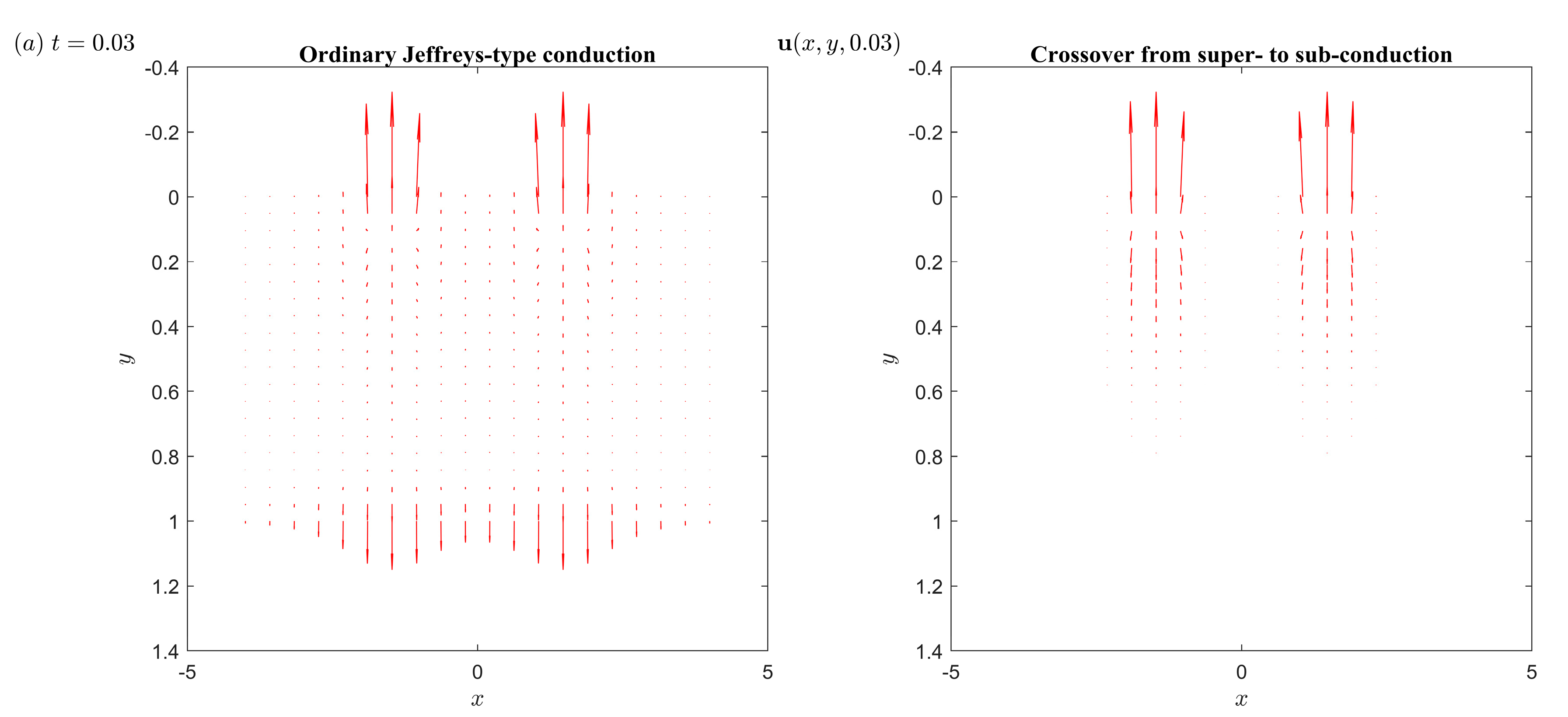
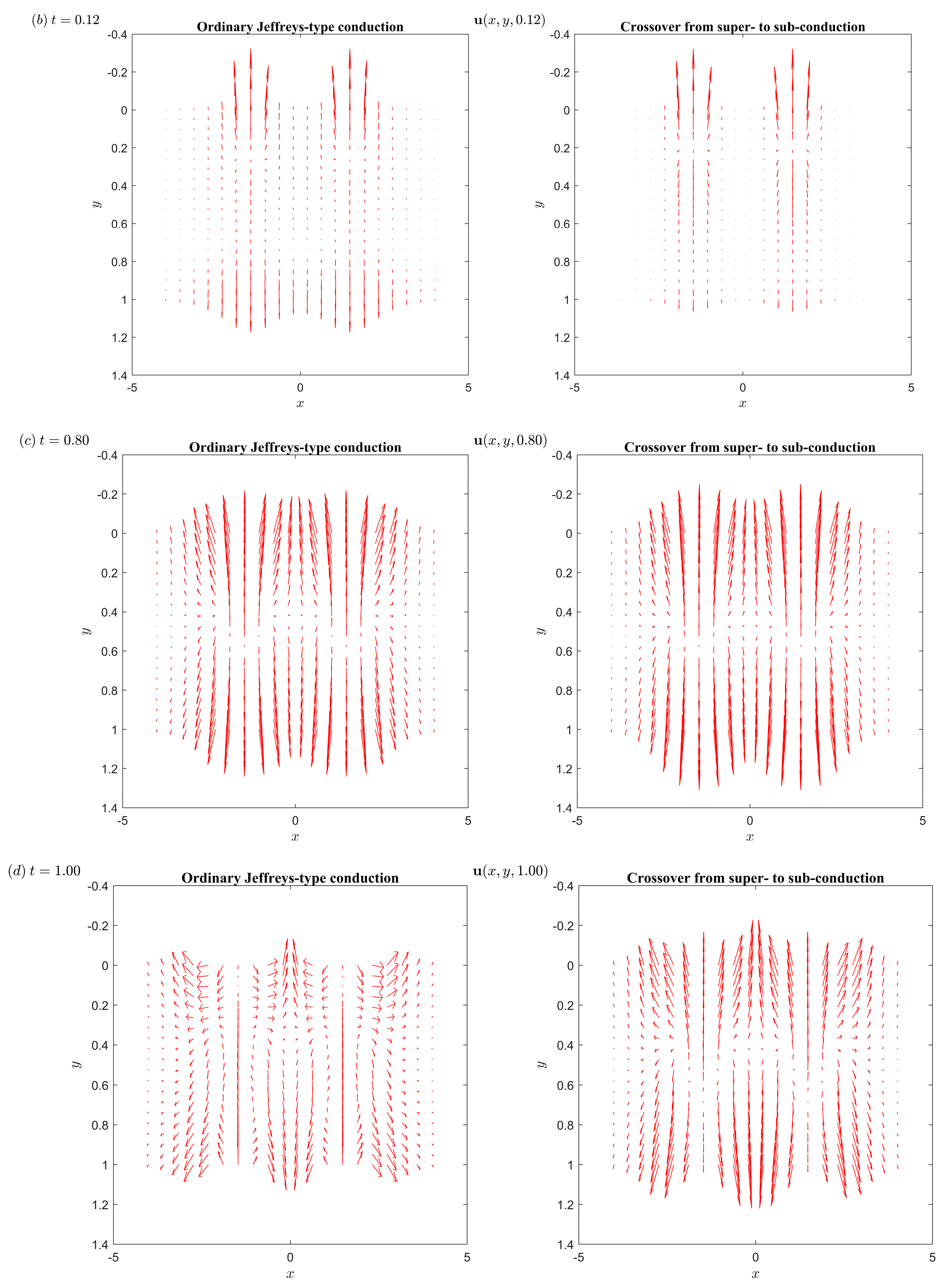
In Figure 8, we represent the displacement vector induced by the ordinary Jeffreys-type heat conduction and the crossover from super- to sub-thermal conduction. We do not attach the other models due to the resemblance between their effects on the displacement with the Jeffreys-type heat conduction and crossover from super- to sub-thermal conduction model. The early arrival of the thermal wave to the lower surface, in the case of a Jeffreys-type heat conductor, is very clear in instant ; see Figure 8a. At the instant , the displacement of the Jeffreys-type heat conduction is on a position of cutting at the double-strip, while the crossover from super- to sub-thermal conduction model is delayed. The contour figures, stress surfaces and displacement vectors are screenshots from full videos in the Supplementary Material section.
6. Summary
In this work, we have studied the effect of anomalous heat transfer inherited from the anomalous diffusion of thermal energy carriers throughout the material lattice. The material response is assumed to follow the Kelvin–Voigt assumption in which the stress–strain relation is not instantaneous; however, there is a retardation in the material strain compared with the elastic “Hookean” response. The Kelvin–Voigt hypothesis may be a reason for the occurrence of anomalies during the diffusion of thermal energy carriers and thus anomalous heat transfer. We have considered a two-dimensional plate with nanoscale thickness, heated by an ultrafast double-strip on its upper surface. The Laplace and Fourier transforms have been used to obtain the solution in the transformed domain. A numerical method based on accelerating the implementation of two infinite sums has been used to obtain the solutions in the proper time–space domain.
The thermal wave resulting from the crossover from super- to sub-thermal conduction is slower than that resulting from the retarded conduction, which in turn is slower than that resulting from the accelerated conduction. The ordinary flux-precedence Jeffreys-type heat conduction has the fastest thermal waves among the models considered in this work. The faster models transport thermal energy to the other surface during a short time interval and record the maximum temperature value on the lower surface. The displacement vector chart of the accelerated and ordinary Jeffreys-type heat conduction evolves faster than those in retarded and crossover models.
Supplementary Materials
The following supporting information can be downloaded at: Video S1: Hydrostatic stress https://youtu.be/Mirfq9-nWVo (accessed on 14 June 2023); Video S2: Temperature contours: https://youtu.be/Eg_V8bakMd4 (accessed on 14 June 2023); Video S3: Displacement of ordinary Jeffreys and crossover: https://youtu.be/tmSBJDmM6-g (accessed on 14 June 2023); Video S4: Displacement for retarded case: https://youtu.be/iB93zQzLEWE (accessed on 14 June 2023); Video S5: Displacement for accelerated case: https://youtu.be/W1nXU-GXvH8 (accessed on 14 June 2023).
Author Contributions
Conceptualization, E.A.; Methodology, E.A., M.A.A. and M.F.; Software, E.A. and M.F.; Validation, E.A.; Formal analysis, E.A. and M.F.; Investigation, M.A.A.; Resources, S.E.A.; Data curation, M.F.; Writing—original draft, E.A., S.E.A. and M.F.; Writing—review & editing, S.E.A. and M.A.A.; Visualization, E.A.; Supervision, E.A. and M.A.A.; Funding acquisition, S.E.A. All authors have read and agreed to the published version of the manuscript.
Funding
This research received no external funding.
Data Availability Statement
Data is contained within the article.
Conflicts of Interest
The authors declare no conflict of interest.
References
- Fournier, D.; Boccara, A. Heterogeneous media and rough surfaces: A fractal approach for heat diffusion studies. Phys. A Stat. Mech. Its Appl. 1989, 157, 587–592. [Google Scholar] [CrossRef]
- Tzou, D.Y.; Chen, J.K. Thermal lagging in random media. J. Thermophys. Heat Transf. 1998, 12, 567–574. [Google Scholar] [CrossRef]
- Choi, S.U.S.; Zhang, Z.G.; Yu, W.; Lockwood, F.E.; Grulke, E.A. Anomalous thermal conductivity enhancement in nanotube suspensions. Appl. Phys. Lett. 2001, 79, 2252–2254. [Google Scholar] [CrossRef]
- Li, B.; Wang, J. Anomalous heat conduction and anomalous diffusion in one-dimensional systems. Phys. Rev. Lett. 2003, 91, 044301. [Google Scholar] [CrossRef] [Green Version]
- Lee, V.; Wu, C.-H.; Lou, Z.-X.; Lee, W.-L.; Chang, C.-W. Divergent and ultrahigh thermal conductivity in millimeter-long nanotubes. Phys. Rev. Lett. 2017, 118, 135901. [Google Scholar] [CrossRef]
- Tzou, D.Y. Macro-to Microscale Heat Transfer: The Lagging Behavior, 2nd ed.; John Wiley & Sons: Hoboken, NJ, USA, 2014. [Google Scholar]
- Compte, A.; Metzler, R. The generalized Cattaneo equation for the description of anomalous transport processes. J. Phys. A Math. Gen. 1997, 30, 7277. [Google Scholar] [CrossRef]
- Barkai, E. Fractional Fokker-Planck equation, solution, and application. Phys. Rev. E 2001, 63, 046118. [Google Scholar] [CrossRef] [Green Version]
- Klafter, J.; Lim, S.; Metzler, R. Fractional Dynamics: Recent Advances; World Scientific: Singapore, 2012. [Google Scholar]
- Sierociuk, D.; Dzieliński, A.; Sarwas, G.; Petras, I.; Podlubny, I.; Skovranek, T. Modelling heat transfer in heterogeneous media using fractional calculus. Phil. Trans. R. Soc. A 2013, 371, 20120146. [Google Scholar] [CrossRef] [Green Version]
- Ji, C.-C.; Dai, W.; Sun, Z.-Z. Numerical Method for Solving the Time-Fractional Dual-Phase-Lagging Heat Conduction Equation with the Temperature-Jump Boundary Condition. J. Sci. Comput. 2018, 75, 1307–1336. [Google Scholar] [CrossRef]
- Ji, C.-C.; Dai, W.; Sun, Z.-Z. Numerical Schemes for Solving the Time-Fractional Dual-Phase-Lagging Heat Conduction Model in a Double-Layered Nanoscale Thin Film. J. Sci. Comput. 2019, 81, 1767–1800. [Google Scholar] [CrossRef]
- Bazhlekova, E.; Bazhlekov, I. Transition from Diffusion to Wave Propagation in Fractional Jeffreys-Type Heat Conduction Equation. Fractal Fract. 2020, 4, 32. [Google Scholar] [CrossRef]
- Awad, E.; Metzler, R. Crossover dynamics from superdiffusion to subdiffusion: Models and solutions. Fract. Calc. Appl. Anal. 2020, 23, 55–102. [Google Scholar] [CrossRef] [Green Version]
- Awad, E.; Sandev, T.; Metzler, R.; Chechkin, A. Closed-form multi-dimensional solutions and asymptotic behaviors for subdiffusive processes with crossovers: I. Retarding case. Chaos Solitons Fractals 2021, 152, 111357. [Google Scholar] [CrossRef]
- Awad, E.; Metzler, R. Closed-form multi-dimensional solutions and asymptotic behaviours for subdiffusive processes with crossovers: II. Accelerating case. J. Phys. A: Math. Gen. 2022, 55, 205003. [Google Scholar] [CrossRef]
- Górska, K.; Horzela, A. Subordination and memory dependent kinetics in diffusion and relaxation phenomena. Fract. Calc. Appl. Anal. 2023, 26, 480–512. [Google Scholar] [CrossRef]
- Liu, L.; Zheng, L.; Chen, Y.; Liu, F. Anomalous diffusion in comb model with fractional dual-phase-lag constitutive relation. Comput. Math. Appl. 2018, 76, 245–256. [Google Scholar] [CrossRef] [Green Version]
- Liu, L.; Feng, L.; Xu, Q.; Chen, Y. Anomalous diffusion in comb model subject to a novel distributed order time fractional Cattaneo–Christov flux. Appl. Math. Lett. 2020, 102, 106116. [Google Scholar] [CrossRef]
- Awad, E. Dual-Phase-Lag in the balance: Sufficiency bounds for the class of Jeffreys’ equations to furnish physical solutions. Int. J. Heat Mass Trans. 2020, 158, 119742. [Google Scholar] [CrossRef]
- Awad, E.; Sandev, T.; Metzler, R.; Chechkin, A. From continuous-time random walks to the fractional Jeffreys equation: Solution and properties. Int. J. Heat Mass Transf. 2021, 181, 121839. [Google Scholar] [CrossRef]
- Hetnarski, R.B.; Ignaczak, J. Generalized thermoelasticity. J. Therm. Stress. 1999, 22, 451–476. [Google Scholar]
- Ignaczak, J.; Ostoja-Starzewski, M. Thermoelasticity with Finite Wave Speeds; Oxford University Press: New York, NY, USA, 2010. [Google Scholar]
- Chandrasekharaiah, D.S. Hyperbolic thermoelasticity: A review of recent literature. Appl. Mech. Rev. 1998, 51, 705–729. [Google Scholar] [CrossRef]
- Povstenko, V.Z. Fractional heat conduction equation and associated thermal stress. J. Therm. Stress. 2005, 28, 83–102. [Google Scholar] [CrossRef]
- Povstenko, Y.Z. Fractional Thermoelasticity; Springer: Berlin/Heidelberg, Germany, 2015. [Google Scholar]
- Sherief, H.H.; El-Sayed, A.M.A.; Abd El-Latief, A.M. Fractional order theory of thermoelasticity. Int. J. Solids Struct. 2010, 47, 269–275. [Google Scholar] [CrossRef]
- Youssef, H.M. Theory of fractional order generalized thermoelasticity. J. Heat Transf. 2010, 132, 061301. [Google Scholar] [CrossRef]
- Ezzat, M.A.; Karamany, A.S.E. Fractional order heat conduction law in magneto-thermoelasticity involving two temperatures. Z. Fur. Angew. Math. Phys. 2011, 62, 937–952. [Google Scholar] [CrossRef]
- Awad, E. On the generalized thermal lagging behavior: Refined aspects. J. Therm. Stress. 2012, 35, 293–325. [Google Scholar] [CrossRef]
- Elhagary, M. Effect of Atangana–Baleanu fractional derivative on a two-dimensional thermoviscoelastic problem for solid sphere under axisymmetric distribution. Mech. Based Des. Struct. Mach. 2021, 51, 3295–3312. [Google Scholar] [CrossRef]
- Sherief, H.H.; Abd El-Latief, A.M.; Fayik, M.A. 2D hereditary thermoelastic application of a thick plate under axisymmetric temperature distribution. Math. Methods Appl. Sci. 2022, 45, 1080–1092. [Google Scholar] [CrossRef]
- Mainardi, F. Fractional Calculus and Waves in Linear Viscoelasticity: An Introduction to Mathematical Models; World Scientific: Singapore, 2010. [Google Scholar]
- Gurtin, M.E.; Sternberg, E. On the linear theory of viscoelasticity. Arch. Ration. Mech. Anal. 1962, 11, 291–356. [Google Scholar] [CrossRef]
- Mukhopadhyay, S. Effects of thermal relaxations on thermoviscoelastic interactions in an unbounded body with a spherical cavity subjected to a periodic loading on the boundary. J. Therm. Stress. 2000, 23, 675–684. [Google Scholar] [CrossRef]
- Youssef, H.M.; Al-Lehaibi, E.A. The vibration of viscothermoelastic static pre-stress nanobeam based on two-temperature dual-phase-lag heat conduction and subjected to ramp-type heat. J. Strain Anal. Eng. Des. 2022, 58, 410–421. [Google Scholar] [CrossRef]
- Abouelregal, A.; Zenkour, A. Fractional viscoelastic Voigt’s model for initially stressed microbeams induced by ultrashort laser heat source. Waves Random Complex Media 2020, 30, 687–703. [Google Scholar] [CrossRef]
- Magaña, A.; Quintanilla, R. On the uniqueness and analyticity of solutions in micropolar thermoviscoelasticity. J. Math. Anal. Appl. 2014, 412, 109–120. [Google Scholar] [CrossRef] [Green Version]
- Fabrizio, M.; Franchi, F.; Nibbi, R. Second gradient Green–Naghdi type thermo-elasticity and viscoelasticity. Mech. Res. Commun. 2022, 126, 104014. [Google Scholar] [CrossRef]
- Sherief, H.H.; Helmy, K.A. A two-dimensional generalized thermoelasticity problem for a half-space. J. Therm. Stress. 1999, 22, 897–910. [Google Scholar]
- Sherief, H.H.; Megahed, F.A. A two-dimensional thermoelasticity problem for a half space subjected to heat sources. Int. J. Solids Struct. 1999, 36, 1369–1382. [Google Scholar] [CrossRef]
- El-Maghraby, N.M. A two-dimensional problem for a thick plate with heat sources in generalized thermoelasticity. J. Therm. Stress. 2005, 28, 1227–1241. [Google Scholar] [CrossRef]
- El-Maghraby, N.M. Two-dimensional thermoelasticity problem for a thick plate under the action of a body force in two relaxation times. J. Therm. Stress. 2009, 32, 863–876. [Google Scholar] [CrossRef]
- Pal, P.; Kanoria, M. Thermoelastic wave propagation in a transversely isotropic thick plate under Green–Naghdi theory due to gravitational field. J. Therm. Stress. 2017, 40, 470–485. [Google Scholar] [CrossRef]
- Kalkal, K.K.; Deswal, S.; Yadav, R. Eigenvalue approach to fractional-order dual-phase-lag thermoviscoelastic problem of a thick plate. IJST-T Mech. Eng. 2019, 43, 917–927. [Google Scholar] [CrossRef]
- Tzou, D.Y.; Beraun, J.E.; Chen, J.K. Ultrafast deformation in femtosecond laser heating. J. Heat Transf. 2002, 124, 284–292. [Google Scholar] [CrossRef]
- Falkovsky, L.A.; Mishchenko, E.G. Electron-lattice kinetics of metals heated by ultrashort laser pulses. J. Exp. Theor. Phys. 1999, 88, 84–88. [Google Scholar] [CrossRef] [Green Version]
- Chen, J.K.; Beraun, J.E.; Tham, C.L. Ultrafast thermoelasticity for short-pulse laser heating. Int. J. Eng. Sci. 2004, 42, 793–807. [Google Scholar] [CrossRef]
- Tzou, D.Y.; Chen, J.K.; Beraun, J.E. Recent development of ultrafast thermoelasticity. J. Therm. Stress. 2005, 28, 563–594. [Google Scholar] [CrossRef]
- Awad, E.; Fayik, M.; El-Dhaba, A. A comparative numerical study of a semi-infinite heat conductor subject to double-strip heating under non-Fourier models. Eur. Phys. J. Plus 2022, 137, 1303. [Google Scholar] [CrossRef]
- Awad, E.; Abo-Dahab, S.M.; Abdou, M.A. Exact solutions for a two-dimensional thermoelectric MHD flow with steady-state heat transfer on a vertical plate with two instantaneous infinite hot suction lines. arXiv 2022, arXiv:2212.01665. [Google Scholar] [CrossRef]
- Awad, E. On the time-fractional Cattaneo equation of distributed order. Phys. A Stat. Mech. Its Appl. 2019, 518, 210–233. [Google Scholar] [CrossRef]
- Gorenflo, R.; Mainardi, F. Fractional calculus. In Fractals and Fractional Calculus in Continuum Mechanics; Springer: Berlin/Heidelberg, Germany, 1997; pp. 223–276. [Google Scholar]
- Duffy, D.G. Transform Methods for Solving Partial Differential Equations; Chapman and Hall/CRC: Portsmouth, UK, 2004. [Google Scholar]
- Callister, W.D.; Rethwisch, D.G. Materials Science and Engineering: An Introduction; Wiley: New York, NY, USA, 2007. [Google Scholar]
- Thomas, L.C. Heat Transfer; Prentice Hall: Hoboken, NJ, USA, 1992. [Google Scholar]
- Fayik, M.; Alhazmi, S.E.; Abdou, M.A.; Awad, E. Transient Finite-Speed Heat Transfer Influence on Deformation of a Nanoplate with Ultrafast Circular Ring Heating. Mathematics 2023, 11, 1099. [Google Scholar] [CrossRef]
- Durbin, F. Numerical inversion of Laplace transforms: An efficient improvement to Dubner and Abate′s method. Comput. J. 1974, 17, 371–376. [Google Scholar] [CrossRef] [Green Version]
- Dubner, H.; Abate, J. Numerical inversion of Laplace transforms by relating them to the finite Fourier cosine transform. J. ACM 1968, 15, 115–123. [Google Scholar] [CrossRef]
- Honig, G.; Hirdes, U. A method for the numerical inversion of Laplace transforms. J. Comput. Appl. Math. 1984, 10, 113–132. [Google Scholar] [CrossRef] [Green Version]
- Press, W.H.; Teukolsky, S.A.; Flannery, B.P.; Vetterling, W.T. Numerical Recipes in Fortran 77: The Art of Scientific Computing, 2nd ed.; Cambridge University Press: Cambridge, UK, 1992; Volume 1. [Google Scholar]
- Rukolaine, S.A.; Samsonov, A.M. Local immobilization of particles in mass transfer described by a Jeffreys-type equation. Phys. Rev. E 2013, 88, 062116. [Google Scholar] [CrossRef] [PubMed] [Green Version]
- Bora, A.; Dai, W.; Wilson, J.P.; Boyt, J.C. Neural network method for solving parabolic two-temperature microscale heat conduction in double-layered thin films exposed to ultrashort-pulsed lasers. Int. J. Heat Mass Transf. 2021, 178, 121616. [Google Scholar] [CrossRef]
- Bora, A.; Dai, W.; Wilson, J.P.; Boyt, J.C.; Sobolev, S. Neural network method for solving nonlocal two-temperature nanoscale heat conduction in gold films exposed to ultrashort-pulsed lasers. Int. J. Heat Mass Transf. 2022, 190, 122791. [Google Scholar] [CrossRef]
Figure 1.
Physical description of the problem.

Figure 2.
Temperature distribution (contours) and heat flux vector (arrows) for the “ordinary flux-precedence Jeffreys model“ at four instants: (a) , (b) , (c) , and (d) .
Figure 2.
Temperature distribution (contours) and heat flux vector (arrows) for the “ordinary flux-precedence Jeffreys model“ at four instants: (a) , (b) , (c) , and (d) .
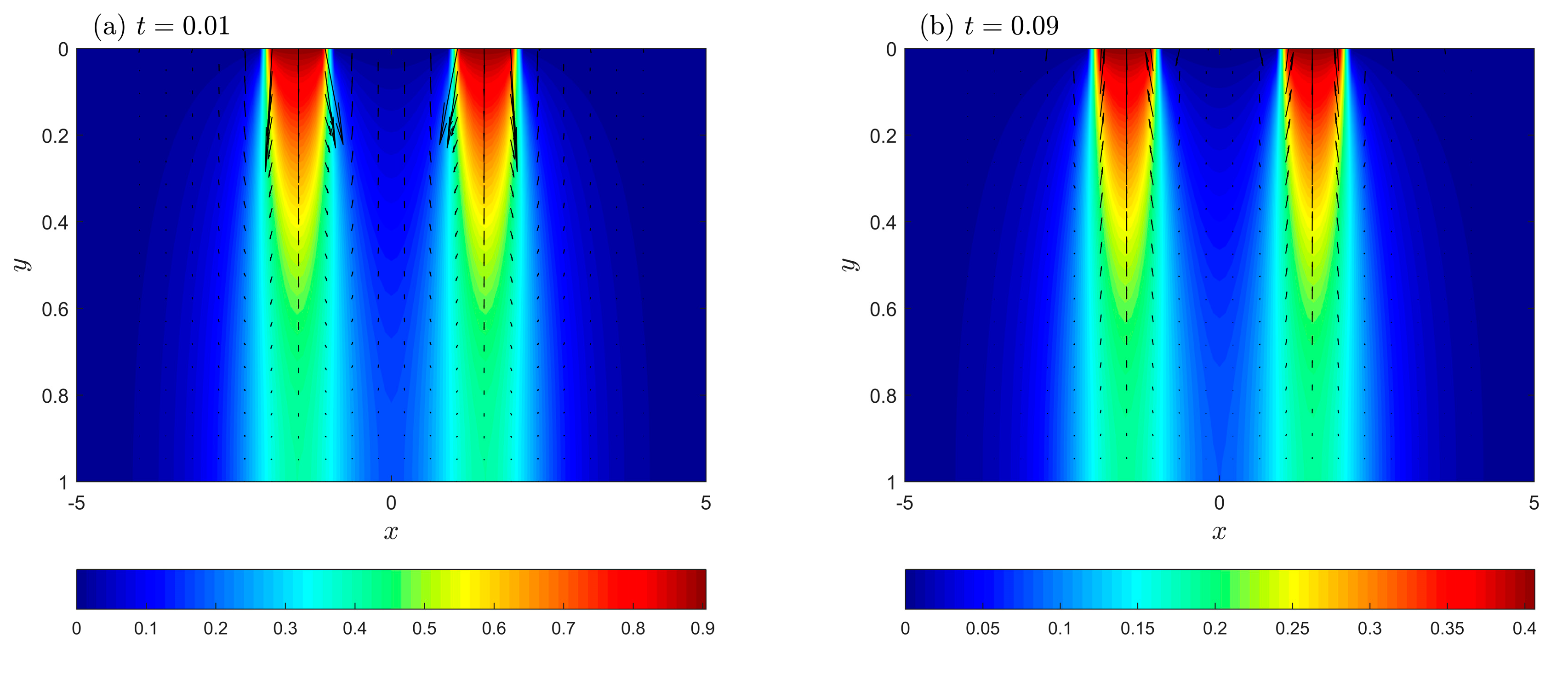

Figure 3.
Temperature distribution (contours) and heat flux vector (arrows) governed by the fractional Jeffreys model with “acceleration” when and , at six instants: (a) , (b) , (c) , (d) , (e) , and (f) .
Figure 3.
Temperature distribution (contours) and heat flux vector (arrows) governed by the fractional Jeffreys model with “acceleration” when and , at six instants: (a) , (b) , (c) , (d) , (e) , and (f) .
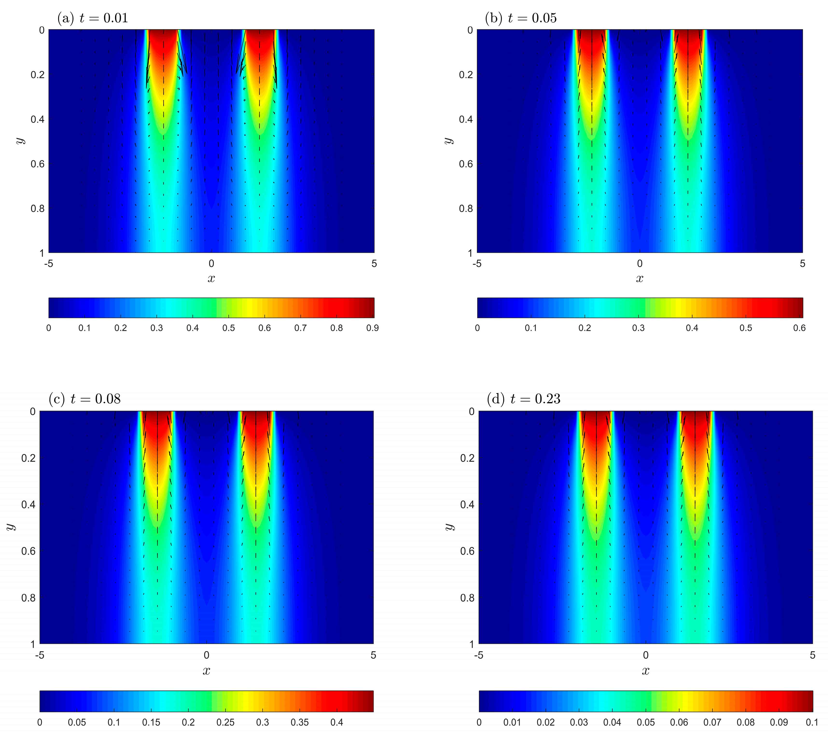

Figure 4.
Temperature distribution (contours) and heat flux vector (arrows) governed by the fractional Jeffreys model with “retardation”, when , , and at six instants: (a) , (b) , (c) , (d) , (e) , and (f) .
Figure 4.
Temperature distribution (contours) and heat flux vector (arrows) governed by the fractional Jeffreys model with “retardation”, when , , and at six instants: (a) , (b) , (c) , (d) , (e) , and (f) .
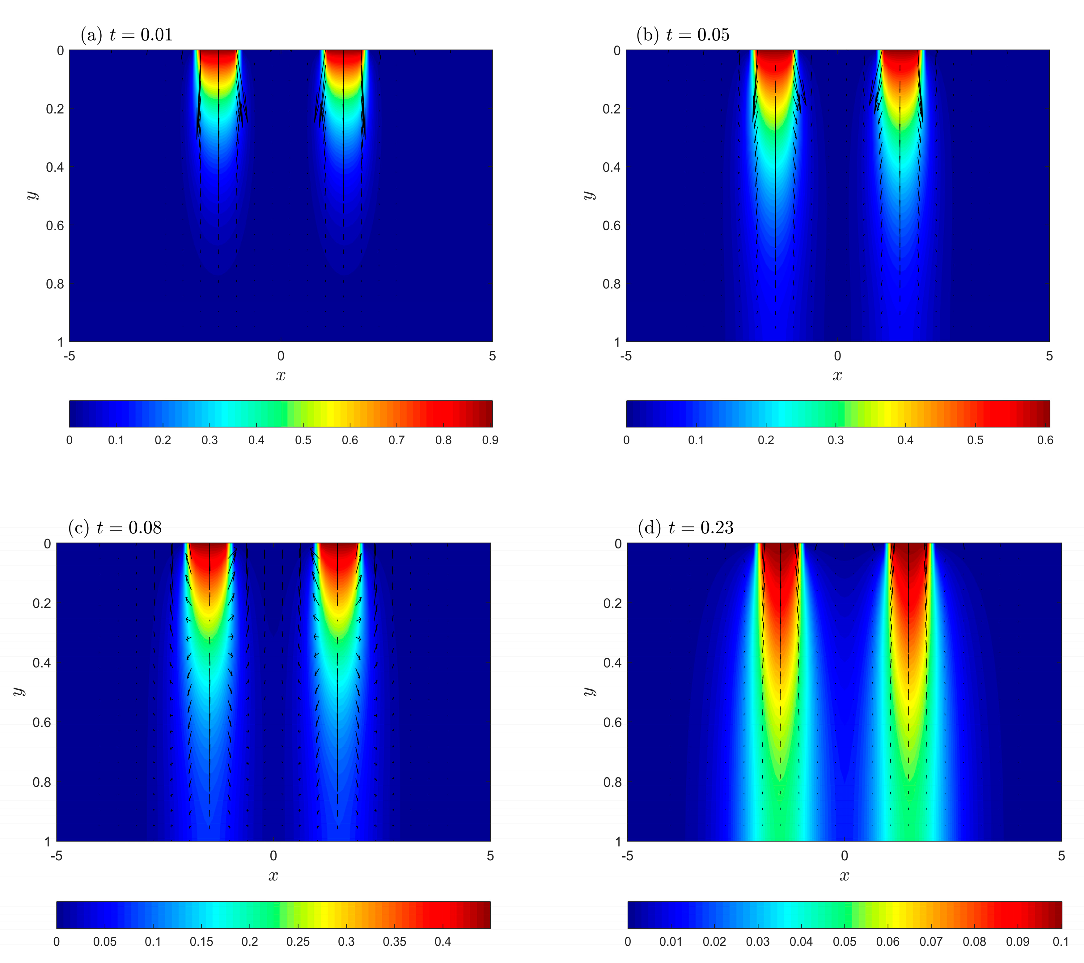
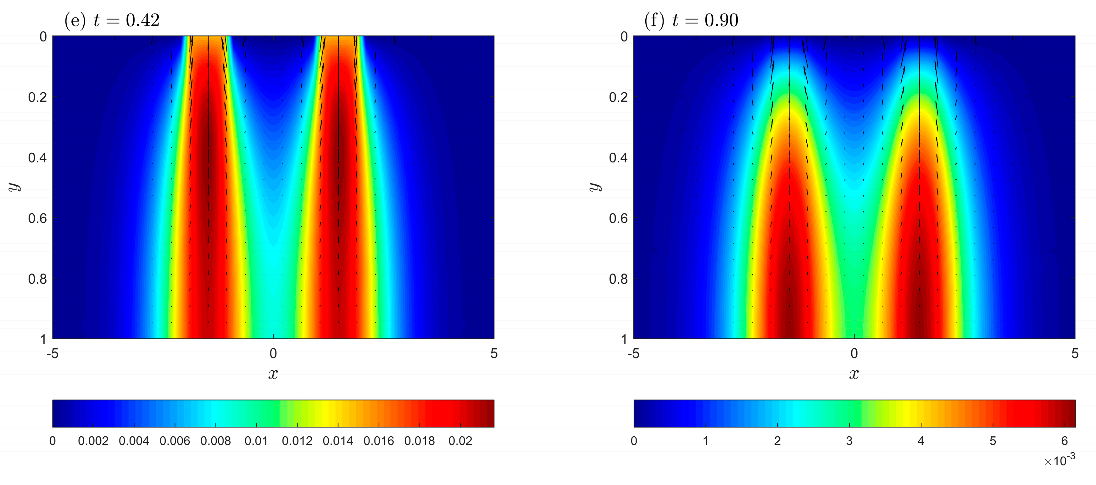
Figure 5.
Temperature distribution (contours) and heat flux vector (arrows) governed by the fractional Jeffreys model with “crossover”, when , , and at six instants: (a) , (b) , (c) , (d) , (e) , and (f) .
Figure 5.
Temperature distribution (contours) and heat flux vector (arrows) governed by the fractional Jeffreys model with “crossover”, when , , and at six instants: (a) , (b) , (c) , (d) , (e) , and (f) .
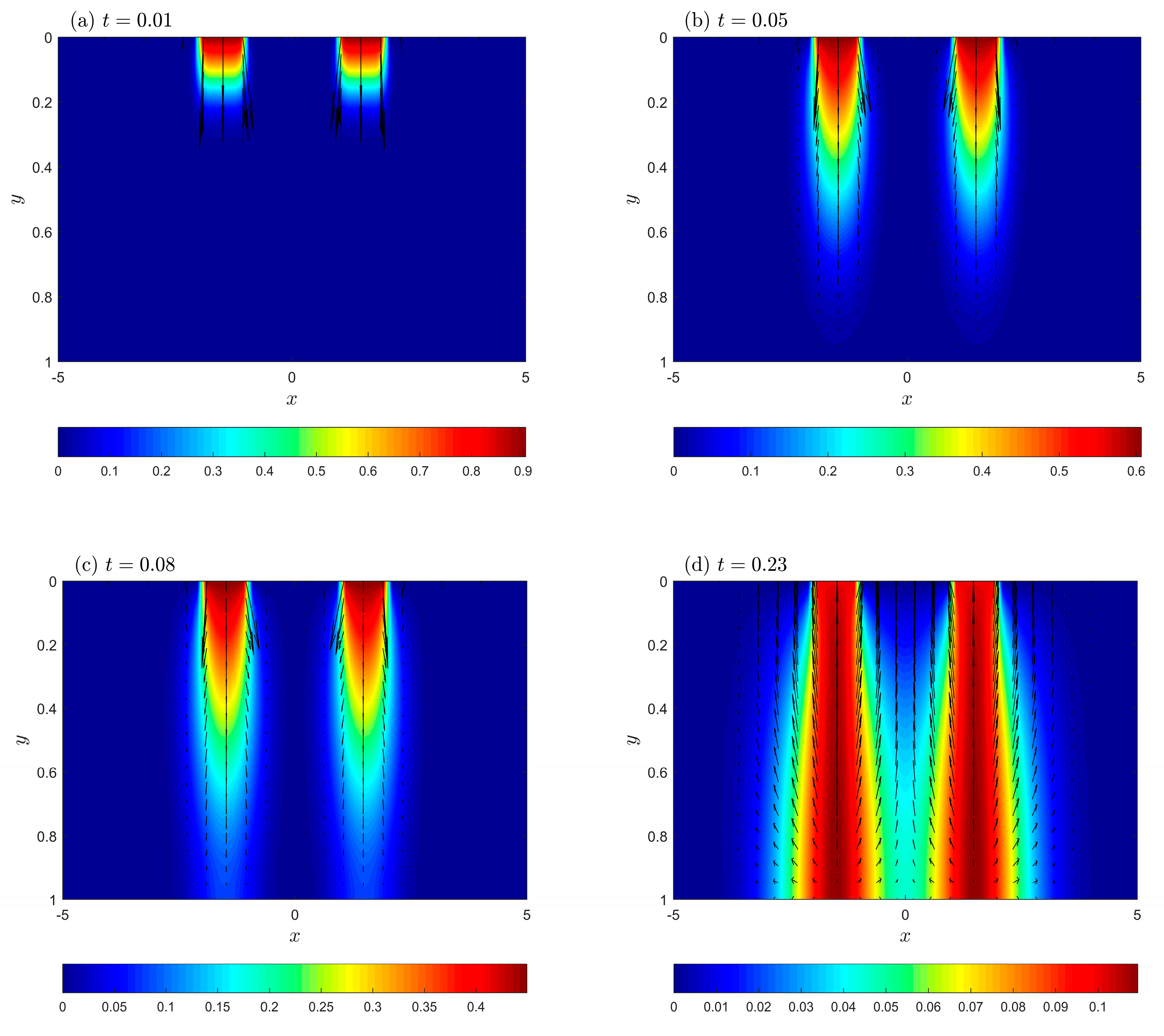
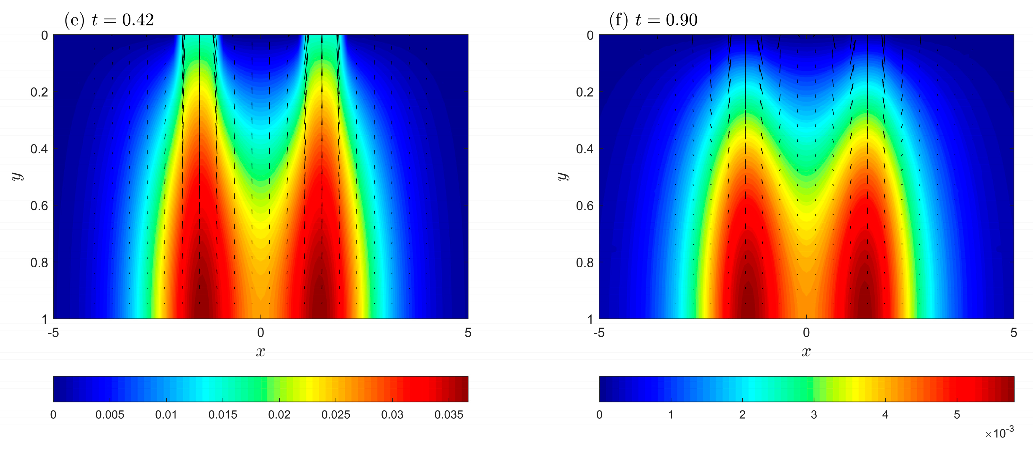
Figure 6.
Hydrostatic stress for the ordinary and fractional flux-precedence Jeffreys model at three instants: (a) , (b) , and (c) .
Figure 6.
Hydrostatic stress for the ordinary and fractional flux-precedence Jeffreys model at three instants: (a) , (b) , and (c) .

Figure 7.
Hydrostatic stress resulting from different Jeffreys-type heat conduction mechanisms at and . (a) Ordinary Jeffreys-type heat conduction, (b) accelerated conduction, (c) retarded conduction, and (d) crossover from super- to sub-thermal conduction.
Figure 7.
Hydrostatic stress resulting from different Jeffreys-type heat conduction mechanisms at and . (a) Ordinary Jeffreys-type heat conduction, (b) accelerated conduction, (c) retarded conduction, and (d) crossover from super- to sub-thermal conduction.
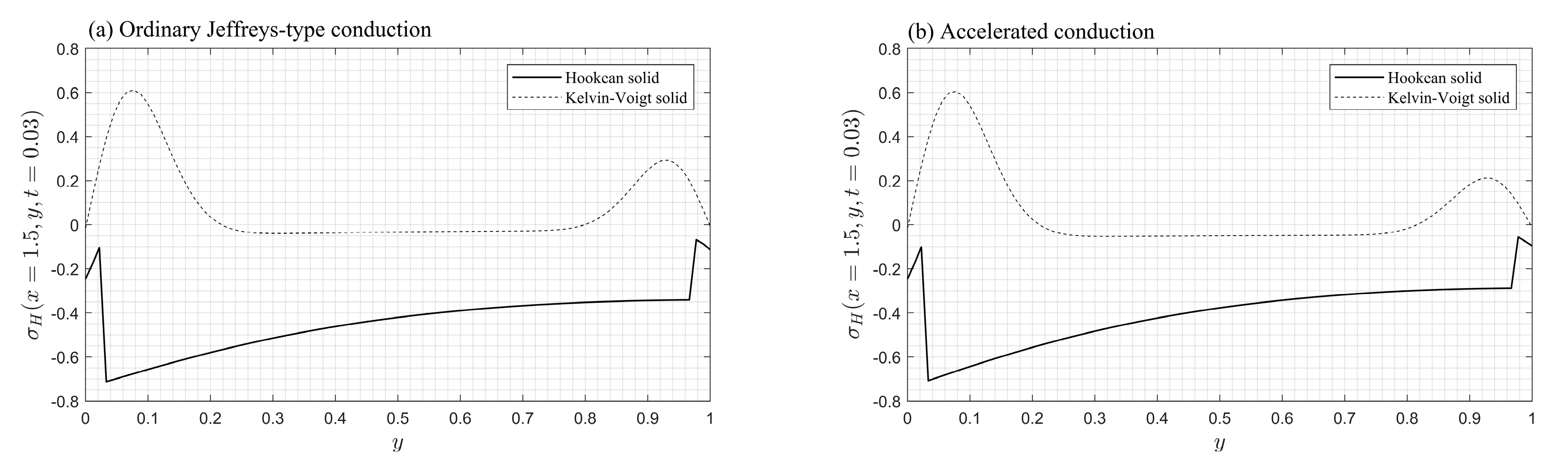
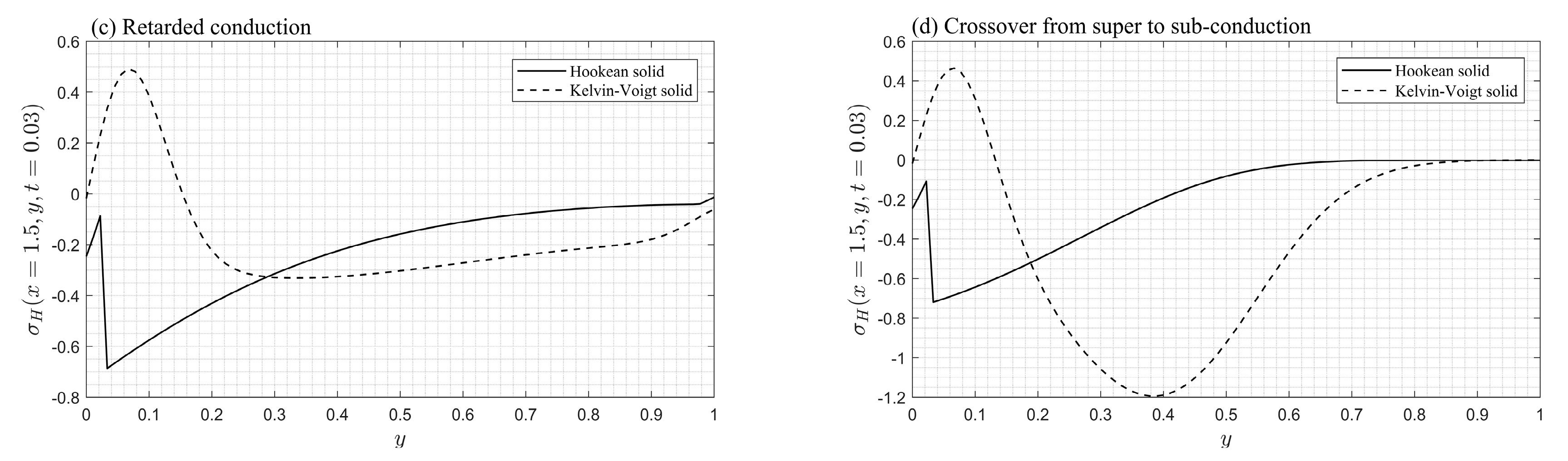
Figure 8.
Displacement vector for the ordinary Jeffreys-type heat conduction and the crossover from super- to sub-thermal conduction models, at four instants: (a) , (b) , (c) , and (d) .
Figure 8.
Displacement vector for the ordinary Jeffreys-type heat conduction and the crossover from super- to sub-thermal conduction models, at four instants: (a) , (b) , (c) , and (d) .

Table 1.
Mechanical and thermal properties of copper at reference temperature .
| Property | |||||||||
|---|---|---|---|---|---|---|---|---|---|
| Value | 8954 | 70.833 | |||||||
| SI unit | picoseconds | picoseconds | picoseconds |
Table 2.
Numerical values of the temperature profile at the dimensionless instant .
| Ordinary Jeffreys Heat Conduction | The Fractional Jeffreys-Type Heat Conduction | ||||||||||||
|---|---|---|---|---|---|---|---|---|---|---|---|---|---|
| Accelerated Conduction | Retarded Conduction | Crossover from Super- to Sub-Conduction | |||||||||||
| x | |||||||||||||
| y | |||||||||||||
| 0.000009 | |||||||||||||
Table 3.
Numerical values of the temperature profile at the dimensionless instant .
| Ordinary Jeffreys Heat Conduction | The Fractional Jeffreys-Type Heat Conduction | ||||||||||||
|---|---|---|---|---|---|---|---|---|---|---|---|---|---|
| Accelerated Conduction | Retarded Conduction | Crossover from Super- to Sub-Conduction | |||||||||||
| x | |||||||||||||
| y | |||||||||||||
| 0.000019 | |||||||||||||
Disclaimer/Publisher’s Note: The statements, opinions and data contained in all publications are solely those of the individual author(s) and contributor(s) and not of MDPI and/or the editor(s). MDPI and/or the editor(s) disclaim responsibility for any injury to people or property resulting from any ideas, methods, instructions or products referred to in the content. |
© 2023 by the authors. Licensee MDPI, Basel, Switzerland. This article is an open access article distributed under the terms and conditions of the Creative Commons Attribution (CC BY) license (https://creativecommons.org/licenses/by/4.0/).
Share and Cite
MDPI and ACS Style
Awad, E.; Alhazmi, S.E.; Abdou, M.A.; Fayik, M. Anomalous Thermally Induced Deformation in Kelvin–Voigt Plate with Ultrafast Double-Strip Surface Heating. Fractal Fract. 2023, 7, 563. https://doi.org/10.3390/fractalfract7070563
AMA Style
Awad E, Alhazmi SE, Abdou MA, Fayik M. Anomalous Thermally Induced Deformation in Kelvin–Voigt Plate with Ultrafast Double-Strip Surface Heating. Fractal and Fractional. 2023; 7(7):563. https://doi.org/10.3390/fractalfract7070563
Chicago/Turabian StyleAwad, Emad, Sharifah E. Alhazmi, Mohamed A. Abdou, and Mohsen Fayik. 2023. "Anomalous Thermally Induced Deformation in Kelvin–Voigt Plate with Ultrafast Double-Strip Surface Heating" Fractal and Fractional 7, no. 7: 563. https://doi.org/10.3390/fractalfract7070563