
A New Technique to Achieve Torsional Anchor of Fractional Torsion Equation Using Conservation Laws

1
Department of Mathematics, Faculty of Basic Sciences, Bozorgmehr University of Qaenat, Qaenat 97619-86844, Iran
2
Department of Mathematical Sciences, Shahrood University of Technology, Shahrood 36199-95161, Iran
3
Department of Mathematical Sciences, University of South Africa (UNISA), Pretoria 0003, South Africa
4
Department of Mathematics and Informatics, Azerbaijan University, Jeyhun Hajibeyli, 71, Baku AZ1007, Azerbaijan
5
Department of Medical Research, China Medical University Hospital, China Medical University, Taichung 110122, Taiwan
6
Department of Basic Sciences, Sari Agricultural Sciences and Natural Resources University, Sari 48181-68984, Iran
*
Author to whom correspondence should be addressed.
Fractal Fract. 2023, 7(8), 609; https://doi.org/10.3390/fractalfract7080609
Submission received: 26 June 2023
/
Revised: 26 July 2023
/
Accepted: 28 July 2023
/
Published: 8 August 2023
(This article belongs to the Special Issue Nonlinear Fractional Differential Equation and Fixed-Point Theory)
Abstract
:The main idea in this research is introducing another approximate method to calculate solutions of the fractional Torsion equation, which is one of the applied equations in civil engineering. Since the fractional order is closed to an integer, we convert the fractional Torsion equation to a perturbed ordinary differential equation involving a small parameter epsilon. Then we can find the exact solutions and approximate symmetries for the alternative approximation equation. Also, with help of the definition of conserved vector and the concept of nonlinear self-adjointness, approximate conservation laws(ACL) are obtained without approximate Lagrangians by using their approximate symmetries. In order to apply the presented theory, we apply the Lie symmetry analysis (LSA) and concept of nonlinear self-adjoint Torsion equation, which are very important in mathematics and engineering sciences, especially civil engineering.
1. Introduction
Fractional calculus is a rapidly developing discipline within mathematics that has gained significant attention in recent years due to its ability to model and understand nonlinear phenomena to various scientific and engineering disciplines. Using new aspects of fractional calculus, researchers can further expand its applications across different disciplines [1]. Over the course of several decades, Lie symmetry analysis (LSA) has been widely applied and demonstrated its significance in various fields, including mathematics, mechanics, dynamics, control theory, and modeling. LSA has proven to be a valuable tool for studying and solving partial differential equations (PDEs) and fractional differential equations (FDEs) [2,3,4]. Recently, many scientists have been applied various methods to obtain analytical solutions of FDEs in different papers such as, the sine-Gordon expansion method [5], first integral method [6], Lie symmetry method [7], Bäcklund transformation method [8], fractional sub-equation method [9], -expansion method [10], extended unified method [11], Yang’s special function method [12] and so on. However, this paper is devoted of approximating FDEs to corresponding ODEs when including small epsilon parameter the fractional order is closed to an integer value [13,14,15,16,17,18]. Solutions of the FDEs can be obtained based on the solutions of the perturbed equations by substituting the original FDE into the approximate differential equation and by approximate with integer order derivative with epsilon parameter.
Conservation laws play a crucial role in the investigation and interpretation of PDEs within the realms of mathematical and engineering sciences. The conserved vectors of conservation laws using LSA can be obtained by new Noether’s operators [19,20,21,22,23,24].
In view of the fact that it is not possible to calculate all the group-invariant solutions, all these invariant solutions can be classified into different classes. By explaining that under the symmetry group, a solution from one class can be transformed to another from the same class. So that the answers of different classes are not the same. This classification of solutions is called the optimal system under the subalgebra [25,26,27].
In solid mechanics, torsion is defined as the twisting of a body due to the applied torque. We consider a uniform rod that is fixed at one end and subjected to torque at the other end. This torque is typically applied about its axis, and it twists the rod to a specific angle. It is assumed that the rod cannot be subjected to compression beyond its elastic limit. In this article, we focus on studying the following Torsion equation with the aim of calculating the applied torsional anchor on edge steel beams in connection with the joist roof and block.
Here is torsional hardness constant and m is torsional anchor constant that cross-sectional area of the beam is in the distance x from the support, and it creates a rotational as much . Since edge beams in steel buildings are affected by bending and torsion anchors due to the load bearing wall and the one-way roof slab attached thereto, it can be assumed that the girder is fully integrated with the roof slab and its lateral period is dependent on the roof slab support period.
The torsional anchor of the wall load can be calculated according to the position on the wing of the edge beam and its deviation from its axis. However, the torsion due to the load of the roof slab connected to the edge beam due to the uncertainty of the exact position of the slab support relative to the weak axis of the beam can not be easily calculated. Therefore, according to the principle of conformity of the deformation between the bending period of the end of the slab and the torsion of the edge beam, it is possible to calculate the period of the slab roof support based on the slab and load characteristics. One can then calculate the torsion anchor on an edge beam whose period is like the roof slab. Obviously, the higher the slab ceiling size, the greater the bending hardness, the lower the slab end time and consequently the edge beam torsion and the torsion on the beam is also reduced.
Our main purpose for this article is to investigate the LSA and solutions to the FTE. We can construct the conservation laws using modified Noether’s theorem [28,29,30,31].
In sequel, we construct the optimal system of subalgebras of the found symmetries for Torsion FDE. This article is organized as follows.
In Section 2, the basic results to convert an FDE to an approximate equation and some definitions are presented. The determining equations and the infinitesimal transformations are obtained in Section 3. In Section 4, some reduced equations and optimal system are obtained. ACL of equation are introduced through the concept of nonlinear self adjointness, and methodology to obtain the ACL of Torsion perturbed FDEs is illustrated in Section 5. Finally, conclusion is given in Section 6.
2. Converting the FDE to Approximate ODE
In the past few decades, FDEs have gained significant popularity as a modeling tool for various physical phenomena. They have found widespread application, particularly in situations where classical calculus fails to efficiently describe uncommon phenomena and complex natural processes. FDEs provide a more flexible and accurate framework for capturing the behavior of these systems, allowing researchers to better understand and predict their dynamics. The first note about fractional derivatives history dates back about 300 years ago. Since then, many mathematicians studied the fractional calculus like Fourier, Liouville, Lacroix, Riemann, Letnikov, Abel, Caputo and many others have all contributed to the advancement of this discipline [32,33,34,35].
We present briefly some definitions and properties of the Caputo and Riemann-Liouville fractional operators which will be used in the further of our work.
There are several different type fractional derivatives. However, we use the right and left hand sides fractional derivatives in the Riemann-Liouville and Caputo sense as follows [17,36,37,38].
Definition 1.
The left and right-sided Caputo fractional partial derivative are defined by
Definition 2.
The left and right-sided Riemann-Liouville fractional partial derivative are defined by
Here and denotes Gamma function.
Let us consider a multi orders FDE as follows:
where and are positive increasing sequences and . Also, is a function of and
are successive derivatives of w.r.t .
3. Lie Group Analysis for Perturbed Equation (12)
Inasmuch as Lie group analysis is an efficient algorithmic approach to study symmetric properties of differential equations so many researchers investigated how to construct approximate symmetries for perturbed equations via this method. Such as Baikov et al., Johnpillai et al. [13,22,23], have applied standard methods of perturbation operator symmetry and dependent variables to obtain approximate symmetries. The first order differential operator is
where
By computing the solutions of the characteristic equation
exact symmetries will be achieved for the perturbed Equation (7).
The approximate point transformations are
that satisfied in
are a one-parameter approximate Lie-point transformation group when the group properties
are satisfied with the accuracy .
4. Classification of Group-Invariant Solution
The construction of optimal system for one dimensional subalgebras reduce to the classification of the orbits for the adjoint representation (AR) [18]. If we know the infinitesimal adjoint action of a Lie algebra on itself, we can reconstruct the adjoint representation of the underlying Lie group, either by integrating the system of linear ordinary differential equations.
with solution
where
Here is a parameter and denotes the usual commutator.
4.1. Optimal System of Perturbed Fractional Torsion Equation
Consider perturbed fractional torsion equation
We must first apply extension (8) for Equation (16) in order to estimate the symmetries of the above perturbed fractional equation.
Let , it leads the approximation of Equation (16) as follows
For this purpose, we should to obtain symmetries of perturbed Equation (17), that results are as follows using Maple 2021.1 software.
In Table 1, Table 2, Table 3 and Table 4, the ARs are given for unperturbed part of (17) By using the infinitesimal generators (18),
where

Table 1.
AR for unperturbed part of Equation (17).
Table 1.
AR for unperturbed part of Equation (17).
| Ad[Xi, Xj] | ||
|---|---|---|
Table 2.
AR for unperturbed part of Equation (17).
Table 2.
AR for unperturbed part of Equation (17).
| Ad[Xi, Xj] | ||
|---|---|---|
Table 3.
AR for unperturbed part of Equation (17).
Table 3.
AR for unperturbed part of Equation (17).
| Ad[Xi, Xj] | ||
|---|---|---|
Table 4.
AR for unperturbed part of Equation (17).
Table 4.
AR for unperturbed part of Equation (17).
| Ad[Xi, Xj] | ||
|---|---|---|
Let be the most general element, and then we will simplify it by applying suitable adjoint maps. Finally, we can obtain the one-dimensional optimal system of (18). The following symmetries are just a few of the members of the one-dimensional optimal system of the perturbed torsion equation, that is given by:
4.2. Reduction and Exact Solution of Perturbed Torsion Equation (18)
Case 1: For the symmetry of , solution of unperturbed part of reduced equation will be in the form
Case 2: For , By using corresponding characteristic equation
and integration of that, invariant solution and reduced equation of unperturbed torsional equation will be in the form:
is solution of above reduced equation.
Case 3: For the reduced equation is:
where is solution of unperturbed equation of the above equation.
Case 4: Symmetry , with invariant function
, and reduced equation
have two solutions in the form:
and
where
and are arbitrary constants.
Case 5: Finally for symmetry , with invariant function and solution similar to case 3.
5. ACL for Equation (12)
We know that the connection between conservation laws and symmetries of the differential equations can be expressed with the Noether’s theorem.
Johnpillai et al. [23] studied about ACL via approximate Noether type symmetry operators.
5.1. Construction of Conservation Laws
Here, we remind the aim of nonlinear self-adjointness of perturbed equations for inducing approximate nonlinear self-adjointness.
For Equation (12), consider formal Lagrangian as follows
Adjoint equations are defined for Equation (12) as follows:
where denotes i th-derivatives of v w.r.to x, is the variational derivative written as
and
If assume
we write
and if Equation (12) satisfies following condition then we called it approximately nonlinearly self adjoint equation
In (22), those parameters and are unknown.
5.2. ACL for Torsion Perturbed Fractional Equation
According to approximate formal Lagrangian
using Equation (20), we obtain adjoint equation as follows:
here
We can obtain an approximate formal Lagrangian by placing (27) into (26) and studying Equation (22), so we get
where and are arbitrary constants.
Then
where
and b are arbitrary constants.
By using the Formulas (23) and (24) and perform all necessary computations, the conserved vector for Equation (16) can be obtained as follows
where
- (I)
- For , , and component of ACL is:
- (II)
- Symmetry , yields and , therefore
- (III)
- For unperturbed symmetry , we obtain and , so we have
- (IV)
- Consider the symmetry , with and , we have
- (V)
- For , , , we have
- (VI)
- For , and , we conclude
- (VII)
- For , and , we obtain
- (VIII)
- Symmetry , gives and , we get
- (VIIII)
- The approximate symmetry with and , yields
- (X)
- Similarly for , and , we derive
- (XI)
- Finally, for , and , we obtain
The torsion constant J for the IPE(a standard related to narrow-flange I-beams) and 2IPE sections is given in Table 5.
6. Conclusions
In this paper, we investigated a method in which a term containing a small epsilon parameter should be replaced the fractional expression of an FDE. Using these terms that approximate with a small parameter, new approximate symmetries, conservation laws of reduced partial differential equations have been found. And then followed by with the help of Lie transformations, analytical solutions, perturbed symmetry and conservation laws of fractional Torsion equation are obtained.
Author Contributions
Conceptualization, methodology and software, N.K.; formal analysis, N.K.; investigation, N.K., H.J., E.L. and Y.K.; writing—original draft preparation, N.K., E.L. and Y.K.; writing—review and editing, H.J., N.K. and Y.K.; supervision, N.K. and H.J. All authors have read and agreed to the published version of the manuscript.
Funding
Bozorgmehr University of Qaenat support for this research under contract number 39196.
Data Availability Statement
Not applicable.
Acknowledgments
The authors would like to acknowledge the financial support of Bozorgmehr University of Qaenat for this research under contract number 39196.
Conflicts of Interest
The authors declare no conflict of interest.
References
- He, J.-H. Fractal calculus and its geometrical explanation. Results Phys. 2018, 10, 272–276. [Google Scholar]
- Hilfer, R. Applications of Fractional Calculus in Physics; World Scientific: Singapore, 2000. [Google Scholar]
- Srivastava, V.K.; Awasthi, M.K.; Tamsir, M. RDTM Solution of Caputo time fractional-order hyperbolic telegraph equation. AIP Adv. 2013, 3, 032142. [Google Scholar]
- Gazizov, R.K.; Kasatkin, A.A.; Lukashchuk, S.Y. Continuous transformation groups of fractional differential equations. Vestn. Usatu 2007, 9, 125–135. [Google Scholar]
- Kadkhoda, N.; Jafari, H. An analytical approach to obtain exact solutions of some space-time conformable fractional differential equations. Adv. Differ. Equ. 2019, 1, 428. [Google Scholar] [CrossRef] [Green Version]
- Lu, B. The first integral method for some time fractional differential equations. J. Math. Anal. Appl. 2012, 395, 684–693. [Google Scholar] [CrossRef] [Green Version]
- Jafari, H.; Kadkhoda, N.; Azadi, M.; Yaghobi, M. Group classification of the time-fractional Kaup-Kupershmidt equation. Sci. Iran. 2017, 24, 302–307. [Google Scholar]
- Kang-Jia, W. Bäcklund transformation and diverse exact explicit solutions of the fractal combined Kdv–mkdv equation. Fractals 2022, 30, 2250189. [Google Scholar]
- Sahoo, S.; Ray, S.S. Improved fractional sub-equation method for (3+1)-dimensional generalized fractional KdV-Zakharov-Kuznetsov equations. Comput. Math. Appl. 2015, 70, 158–166. [Google Scholar]
- Guner, O.; Atik, H.; Kayyrzhanovich, A.A. New exact solution for space-time fractional differential equations via -expansion method. Optik 2017, 130, 696–701. [Google Scholar] [CrossRef]
- Osman, M.S. Multiwave solutions of time-fractional (2+1)-dimensional Nizhnik-Novikov-Veselov equations. Pramana J. Phys. 2017, 88, 67–75. [Google Scholar]
- Kang-Jia, W.; Feng, S.; Jing, S.; Jing-Hua, L.; Guo-Dong, W. Non-differentiable exact solutions of the local fractional zakharov–kuznetsov equation on the cantor sets. Fractals 2023, 31, 2350028. [Google Scholar]
- Baikov, V.A.; Gazizov, R.K.; Ibragimov, N.H. Perturbation methods in group analysis. J. Sov. Math. 1991, 55, 1450–1490. [Google Scholar] [CrossRef]
- Euler, M.; Euler, N.; Kohler, A. On the construction of approximate solutions for a multi-dimensional nonlinear heat equation. J. Phys. A Math. Gen. 1994, 27, 2083–2092. [Google Scholar] [CrossRef]
- Kara, A.F.; Mahomed, F.M.; Qu, C.Z. Approximate potential symmetries for partial differential equations. J. Phys. Math. Gen. 2000, 33, 6601–6613. [Google Scholar] [CrossRef]
- Habibi, N.; Lashkarian, E.; Dastranj, E.; Hejazi, S.R. Lie symmetry analysis, conservation laws and numerical approximations of time-fractional Fokker-Planck equations for special stochastic process in foreign exchange markets. Physical A 2019, 513, 750–766. [Google Scholar] [CrossRef]
- Mahomed, F.M.; Qu, C.Z. Approximate conditional symmetries for partial differential equations. J. Phys. Math. Gen. 2000, 33, 343–356. [Google Scholar] [CrossRef]
- Kadkhoda, N.; Lashkarian, E.; Inc, M.; Akinlar, M.A.; Chu, Y.M. New exact solutions and conservation laws to the fractional-order Fokker–Planck equations. Symmetry 2020, 12, 1282. [Google Scholar] [CrossRef]
- Ibragimov, N.H. Nonlinear self-adjointness in constructing conservation laws. J. Phys. Math. Theor. 2011, 7, 432002. [Google Scholar] [CrossRef]
- Ibragimov, N.H.; Kovalev, V.F. Approximate and Renormgroup Symmetries. In Nonlinear Physical Science, 1st ed.; Springer: New York, NY, USA, 2009. [Google Scholar]
- Johnpillai, A.G.; Kara, A.H. Variational Formulation of Approximate Symmetries and Conservation Laws. Int. J. Theor. Phys. 2001, 40, 1501–1509. [Google Scholar] [CrossRef]
- Johnpillai, A.G.; Kara, A.H.; Mahomed, F.M. A basis of approximate conservation laws for PDEs with a small parameter. Int. J. Nonlinear Mech. 2006, 41, 830–837. [Google Scholar] [CrossRef]
- Johnpillai, A.G.; Kara, A.H.; Mahomed, F.M. Approximate Noether type symmetries and conservation laws via partial Lagrangians for PDEs with a small parameter. J. Comput. Appl. Math. 2009, 223, 508–518. [Google Scholar]
- Kara, A.H.; Mahomed, F.M.; Unal, G. Approximate Symmetries and Conservation Laws with Applications. Int. J. Theor. Phys. 1999, 38, 2389–2399. [Google Scholar] [CrossRef]
- Buckwar, E.; Luchko, Y. Invariance of a partial differential equation of fractional order under the Lie group of scaling transformations. J. Math. Anal. Nand Appl. 1998, 227, 81–97. [Google Scholar] [CrossRef] [Green Version]
- Ibragimov, N.H. Transformation Groups Applied to Mathematical Physics; Reidel, D., Ed.; Springer: Berlin/Heidelberg, Germany, 1985. [Google Scholar]
- Olver, J.P. Application of Lie Groups to Differential Equations; Springer: New York, NY, USA, 1986. [Google Scholar]
- Lukashchuk, S.Y. Conservation laws for time-fractional subdiffusion and diffusion-wave equations. Nonlinear Dyn. 2015, 80, 791–802. [Google Scholar] [CrossRef] [Green Version]
- Lukashchuk, S.Y. Constructing conservation laws for fractional order integro-differential equations. Theor. Math. Phys. 2015, 184, 1049–1066. [Google Scholar] [CrossRef]
- Hejazi, S.R.; Hosseinpour, S.; Lashkaian, E. Approximate symmetries, conservation laws and numerical solutions for a class of perturbed linear wave type system. Quaest. Math. 2019, 10, 1391–1409. [Google Scholar]
- Lukashchuk, S.Y. Approximate conservation laws for fractional differential equations. Commun. Nonlinear Sci. Numer. Simul. 2019, 68, 147–159. [Google Scholar]
- Mainardy, F. Fractional Calculus and Waves in Linear Viscoelasticity, An Introduction to Mathematical Models; Imperial College Press: Singapore, 2010. [Google Scholar]
- Sabatier, J.; Agrawal, O.P.; Machado, J.A.T. Advances in Fractional Calculus, Theoretical Developments and Applications in Physics and Engineering; Springer: Dordrecht, The Netherlands, 2007. [Google Scholar]
- Samko, S.; Kilbas, A.; Marichev, O. Fractional Integrals and Derivatives: Theory and Applications; Gordon and Breach Science Publisers: London, UK, 1993. [Google Scholar]
- Zhou, Y.; Wang, J.; Zhang, L. Basic Theory of Fractional Differential Equations; World Scientific: London, UK, 2016. [Google Scholar]
- Kilbas, A.A.; Srivastava, H.M.; Trujillo, J.J. Theory and Applications of Fractional Differential Equations; Elsevier: Amsterdam, The Netherlands, 2006. [Google Scholar]
- Kiryakova, V. Generalised Fractional Calculus and Applications; CRC Press: Boca Raton, FL, USA, 1994; Volume 301. [Google Scholar]
- Podlubny, I. Fractional Differential Equations: An Introduction to Fractional Derivatives, Fractional Differential Equations, to Methods of Their Solution and Some of Their Applications; Academic Press: New York, NY, USA, 1999. [Google Scholar]
Figure 1.
= 1.

Figure 2.
= 1.
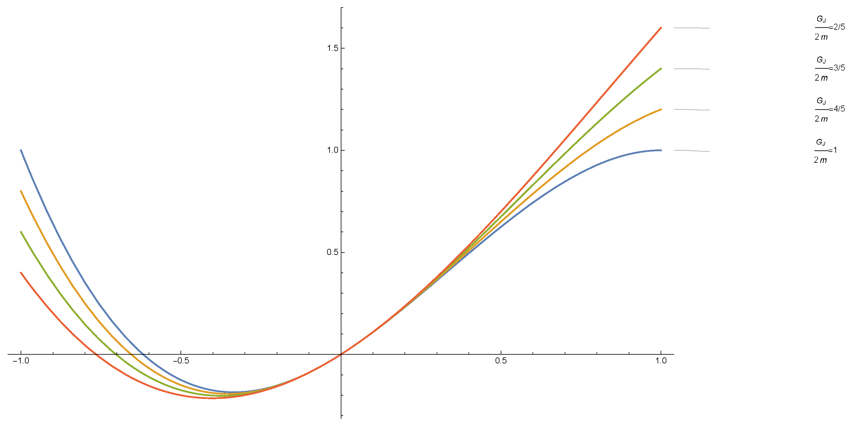
Table 5.
The torsion constant J.
| PE | J | 2PE | J |
|---|---|---|---|
| 140 | |||
| 160 | |||
| 180 | |||
| 200 | |||
| 220 | |||
| 240 | |||
| 270 | |||
| 300 | |||
| 330 | |||
| 370 | |||
| 400 |
Disclaimer/Publisher’s Note: The statements, opinions and data contained in all publications are solely those of the individual author(s) and contributor(s) and not of MDPI and/or the editor(s). MDPI and/or the editor(s) disclaim responsibility for any injury to people or property resulting from any ideas, methods, instructions or products referred to in the content. |
© 2023 by the authors. Licensee MDPI, Basel, Switzerland. This article is an open access article distributed under the terms and conditions of the Creative Commons Attribution (CC BY) license (https://creativecommons.org/licenses/by/4.0/).
Share and Cite
MDPI and ACS Style
Kadkhoda, N.; Lashkarian, E.; Jafari, H.; Khalili, Y. A New Technique to Achieve Torsional Anchor of Fractional Torsion Equation Using Conservation Laws. Fractal Fract. 2023, 7, 609. https://doi.org/10.3390/fractalfract7080609
AMA Style
Kadkhoda N, Lashkarian E, Jafari H, Khalili Y. A New Technique to Achieve Torsional Anchor of Fractional Torsion Equation Using Conservation Laws. Fractal and Fractional. 2023; 7(8):609. https://doi.org/10.3390/fractalfract7080609
Chicago/Turabian StyleKadkhoda, Nematollah, Elham Lashkarian, Hossein Jafari, and Yasser Khalili. 2023. "A New Technique to Achieve Torsional Anchor of Fractional Torsion Equation Using Conservation Laws" Fractal and Fractional 7, no. 8: 609. https://doi.org/10.3390/fractalfract7080609