New Cascaded 1+PII2D/FOPID Load Frequency Controller for Modern Power Grids including Superconducting Magnetic Energy Storage and Renewable Energy

Abstract

Having continuous decrease in inertia and being sensitive to load/generation variation are considered crucial challenging problems for modern power grids. The main cause of these problems is the increased penetration capacities of renewables. An unbalanced load with generation power largely affects grids’ frequency and voltage profiles. Load frequency control (LFC) mechanisms are extensively presented to solve these problems. In the literature, LFC methods are still lacking in dealing with system uncertainty, parameter variation, structure changes, and/or disturbance rejection. Therefore, this paper proposes an improved LFC methodology using the hybrid one plus proportional integral double-integral derivative (1+PII2D) cascaded with fractional order proportional-integral-derivative (FOPID), namely, the proposed 1+PII2D/FOPID controller. The contribution of superconducting magnetic energy storage devices (SMES) is considered in the proposed design, also considering hybrid high-voltage DC and AC transmission lines (hybrid HVDC/HVAC). An optimized design of proposed 1+PII2D/FOPID controller is proposed using a new application of the recently presented powerful artificial rabbits optimizers (ARO) algorithm. Various performance comparisons, system changes, parameter uncertainties, and load/generation profiles and changes are considered in the proposed case study. The results proved superior regulation of frequency using proposed 1+PII2D/FOPID control and the ARO optimum parameters.

1. Introduction

Transition in energy-related sectors to new renewable energy sources (RESs) has become mandatory due to climate changes and limited access to fossil fuel resources. The RESs-based power sources have proven to be excellent candidates with lower levelized cost of energy (LCOE) and are available everywhere without affecting the surrounding environments [1,2]. However, the progress of modern power grids suffers from the following crucial problems:

• A critical characteristic of RESs is their intermittency and related variations of generated power with environmental conditions, such as irradiance, temperature, and wind speeds. For instance, outputted power from photovoltaic (PV) generations is not available during night and shading-effect times. It also varies from one instant to the other during the daytime with changes in solar irradiance and temperatures [3,4].
• Additionally, adding more RES installations in power grids leads to continuous reductions of power systems’ inertia. The inertia is the determining factor of grid stability and robustness. The main reason behind reduced values of inertia is the characteristics of outputted voltage/current of RESs, which cannot be connected directly to power grids. A power electronic power conversion unit is needed to provide adequate voltage/current and power quality waveforms to power grids. These structures are different from conventional energy systems which are based on synchronous generators and the conversion unit helps preserve system stability and robustness. This functionality does not exist in power electronics-based RES generations [5,6].
• Another uncertainty comes from the characteristics of modern connected loads. They are subject to various changes in large steps. Thence, jointly with uncertain RES generation, modern power grids can exhibit severe instabilities and improper responses with step changes in loads/generation and their associated imbalance [7].
• Energy storage systems (ESSs) have become essential for modern power grid with RES power’s variations. They can be used for storing/supplying energy based on the variations in generation/load imbalance. Thence, proper control and management algorithms are needed to provide better utilization of ESSs and to provide support of modern power grids [8].

The control methodology and design of various connected elements of power grids determine to a great extent the system response, behavior, stability, efficiency, and robustness [5]. Load frequency controllers (LFCs) have proven to be a powerful means for controlling and regulating the frequency response of modern power grids considering the aforementioned properties. The LFC can also control tie-line power variations and control the contribution of connected devices in a centralized or distributed way. The literature has presented several control methodologies and design methods for several structure case studies. The structures include the type of conventional generation resources, the load types, the connected RESs, the ESS devices, connected flexible AC transmission system (FACTS) devices, and transmission line structures [7]. Moreover, the applied design methodologies of LFC and other existing controllers in modern power grids determine the system response against various existing disturbances. Compared to mathematically based design approaches in the literature, the employment of metaheuristic optimization algorithms in designing LFCs in grid systems provides simple procedures, simultaneous tuning, no need for complex control theories, and flexible adjustment of desired response through the employed objective functions [4].

A variety of LFC methodologies have been proposed in the literature for regulating frequency in several applications [9]. Recently, advanced and intelligent control methods have been proposed for LFC, such as the model-based predictive controller (MPC), the adaptive neurofuzzy interface system (ANFIS), the artificial neural networks (ANNs), deep neural networks (DNNs), and fuzzy logic-based controllers (FLCs) [10]. In [11], MPC-based grid stabilization considering wind generation has been proposed. Another ANFIS LFC method has been applied to a multi-RES case study and the ant-lion optimization algorithm is used for designing the controller [12]. The ANN LFC has been presented in [13] for solar PV power plants. A hybrid FLC and fractional order (FO) method has been provided in [14] for two interconnected microgrids with PV and wind generations. The wild-horse optimization (WHO) algorithm is used for designing the presented controller. It has shown reduced overshoot values, lower settling times, and good system response. The marine predators algorithm (MPA) has been presented with FLC-based proportional-integral-derivative (PID) in [15]. Another FLC PID with sine-cosine optimizer algorithm (SCA) has been introduced in [16]. The FOPID FLC frequency regulation has been provided with differential evolution-based optimization algorithms (DE) in [17].

A comparison between advanced and classical LFC has been made in [18]. Advanced techniques can achieve improved stability of modern power grids. However, they rely on expert systems and a huge amount of tuning data during their design process. In addition, they need high computational power and processors for optimizing their design and implementation process. On the other hand, classical integer order (IO)- and FO-based control schemes are still experiencing wide interest due to their simplicity, being easy to understand and widely applied in the literature with confirmed superior performance and a wide variety of design algorithms [19]. In [20,21], several IO LFC schemes based on PI, IDD, and PID schemes have been presented. Some optimization algorithms have been associated with IO LFC for optimizing the design, such as Harris Hawks optimizer (HHO) [20], imperialist-competitive algorithms (ICA) [22], artificial bee-colony (ABC) [23], Jaya-Balloon optimizers (JBO) [24], and Electro-Searching Optimizer (ESO) with Balloon Effects (BE) [21].

Virtual inertia control and green hydrogen systems have been presented in [25] for improving the inertial response of power grids. A nonlinear PI controller has been presented in [26], and it is optimized using the dandelion optimization (DO) algorithm for a single area power grid. The particle swarm optimization (PSO) algorithm has been applied in [27] for designing the I and PI for LFC and virtual inertia controller (VIC), respectively, in interconnected microgrids. The IO LFC methods showed simple structures, less complexity, and simple design procedures, and required low cost implementations. However, they cannot fully-mitigate grid fluctuations, are sensitive to parameter changes, and have low design freedom. Two recent applications of artificial rabbits optimizer (ARO) algorithm for control design have been presented in [28,29]. In [28], ARO has been applied for designing the conventional PI and PID controllers in multi-sourced microgrid systems. In [29], the PD-PID accelerated controller has been designed using ARO for static synchronous-compensators (STATCOM) in power systems. Another Fuzzy PIDD2 controller has been presented with the Gradient-Based Optimizer (GBO) algorithm in [30] for stabilizing combined voltage-frequency loops for two-area-based interconnected grids.

Cascaded control schemes used to form outer and inner control loops have been proposed in the literature for achieving better disturbance rejections. In [31], a PD-PI cascaded controller was proposed and it was optimized using enhanced slime mould optimizations algorithm (ESMOA). The two-degrees of freedom (2DOF) PID has been presented in [32] with using the teaching–learning based optimizer (TLBO), whereas the cascaded PD-PID has been presented in [33] and the bat optimization algorithm (BA) has been applied for optimizing the control parameters. In [34], PI-PDF LFC and driver training-based optimizer (DTBO) has been proposed. The above-mentioned LFC schemes have proven better rejection for existing disturbances and hence better stability can be obtained.

More flexibility and higher DOF have been presented in the literature through applying FO control theories with their inherently included FO operators. A FOPID optimized with SCA has been proposed in [35] and movable damped-wave optimization algorithm (MDWA) has been proposed in [36]. FOPID with filter (FOPIDF) has been introduced in [37] for LFC with including additional filtering stage in derivative path. The hybrid TFOID optimized with artificial ecosystem optimization algorithm (AEO) has been proposed in [38] with merging FOPID and TID performance. The FOPID accelerated controller (FOPIDA) has been proposed in [39] for hybrid maritime microgrid systems. The gray-wolf optimization (GWO) has been employed in obtaining the optimum parameters. A proposal of the intelligent FOI (iFOI) controller optimized with GWO has been presented in [40]. Another new combination of TID and FOPID has been presented as a combined TFOID controller for LFC application [41]. The slime mould optimizer algorithm (SMA) has been presented for optimizing the control parameters. Two modified versions of manta ray foraging optimizations algorithm (MRFO) using chaotic map, and the weighting factor (named CMRFO and WCMRFO) have been proposed in [42] for EV-based interconnected microgrids. A coordination strategy between protection devices and TFOID with PI as virtual inertia controller has been provided in [43], in which the SMA has been proposed for optimizing the employed control schemes.

A 3DOF-based TID has been proposed in [44] using three feedback signals. The squirrel searching algorithm (SSA) has been introduced for determining the control parameters. Other examples for cascaded LFC include FO-IDF [45], cascaded PI-TDF [46], and TID [7] have been also presented in the literature. A cascaded FOPI-IDDF LFC scheme optimized with the crow search algorithm (CSA) has been presented in [47] with solar-thermal generation-based grids. Another cascased 1+PD/FOPID LFC method has been proposed in [48] for EV-based power grids, whereas the MRFO has been applied for optimizing the various parameters of the presented controller. The 3DOF cascaded LFC using FOTPID-TIDF control has been presented in [49]. A scaling-chaotic based MRFO (SCMRFO) has been proposed for the design optimization process of the presented controller. The inclusion of three different sensed signals with extra added FO terms lead to improving the frequency regulation performance. However, this controller suffers from increased complexity in its design and in its implementation. A TID-based superconducting-energy storage system (SMES) has been presented in [50] for providing proper virtual inertia with using MRFO for designing the controller. The TID has been used separately for SMES and a separate controller has been proposed for the LFC function. The inclusion of additional integral/derivative/tilt FO operators leads to increasing the control flexibility and DOF for optimizing the power grid response and metrics.

Stimulated by the above-mentioned frequency regulation problems in modern RES microgrids and the need for continuous development of LFC, this paper presents an improved cascaded hybrid controller and it is designed using a new application of a new optimizer algorithm. A comprehensive comparison of existing work in the literature compared with the proposed contribution is presented in Table 1. Although the ARO has been presented in [28,29] for control design, it has not yet been applied for FO control design and cascaded FO control systems with considering the characteristics of SMES, connected RESs, and loads. The main contributions of this paper are summarized as:

Table 1. Summary and comparison of the existing LFC schemes compared with the proposed contribution.

Ref.	Controller	Algorithm	Category	Characteristics of Each Category
[20]	PI	HHO		Use simple control structures
[21]	I	ESO with BE	IO-based	Are easy to implement
[22]	PID	ICA	LFC with	Lower control robustness with parameter uncertainty
[23]	PID	ABC	single input	Have low mitigation ability of disturbances
[24]	I	JBO
[25]	PID	–
[28]	PI, PID	ARO
[26]	Nonlinear PI	DO
[27]	I, PI	PSO
[30]	Fuzzy PIDD2	GBO
[40]	iFOI	GWO
[35]	FOPID	SCA		Have more parameters to tune
[36]	FOPID	MDWA	FO-based	Possess higher flexibility compared to IO ones
[37]	FOPIDF	ICA	LFC with	Have improved disturbance mitigation compared to IO
[38]	TFOID	AEO	single input	Have reduced rejection of existing disturbances
[50]	TID	MRFO
[39]	FOPIDA	GWO
[41]	TFOID	SMA
[42]	TFOID	CMRFO, WCMRFO
[43]	TFOID with PI	SMA
[31]	PD-PI	ESMOA		Possess high number of parameters to tune
[32]	2DOF PID	TLBO	Cascaded LFC	Have more flexibilities (degree of freedom) in design
[33]	PD-PID	BA	with multiple	Provide better disturbance mitigation due to using cascaded loops
[34]	PI-PDF	DTBO	inputs	can mitigate high as well as low frequency disturbances
[44]	3DOF TID	SSA		Have better performance than single input LFC methods
[45]	FO-IDF	ICA
[46]	PI-TDF	SSA
[29]	PD-PIDA (STATCOM)	ARO
[47]	FOPI-IDDF	CSA
[48]	1+PD/FOPID	MRFO
[49]	3DOF FOTPID-TIDF	SCMRFO
Proposed	cascaded 1+PII2D/FOPID	ARO	Cascaded FO LFC (multiple inputs)	A robust new improved hybrid controller The proposed cascaded 1+PII2D/FOPID has two loops that lead to having better rejection possibility of disturbances Applies the recently-presented powerful artificial rabbits optimizers (ARO) algorithm Studies the employment of SMES to contribute in frequency regulation using the proposed 1+PII2D/FOPID controller Studies the behavior of real wind and PV profiles with different domestic and industrial load profiles

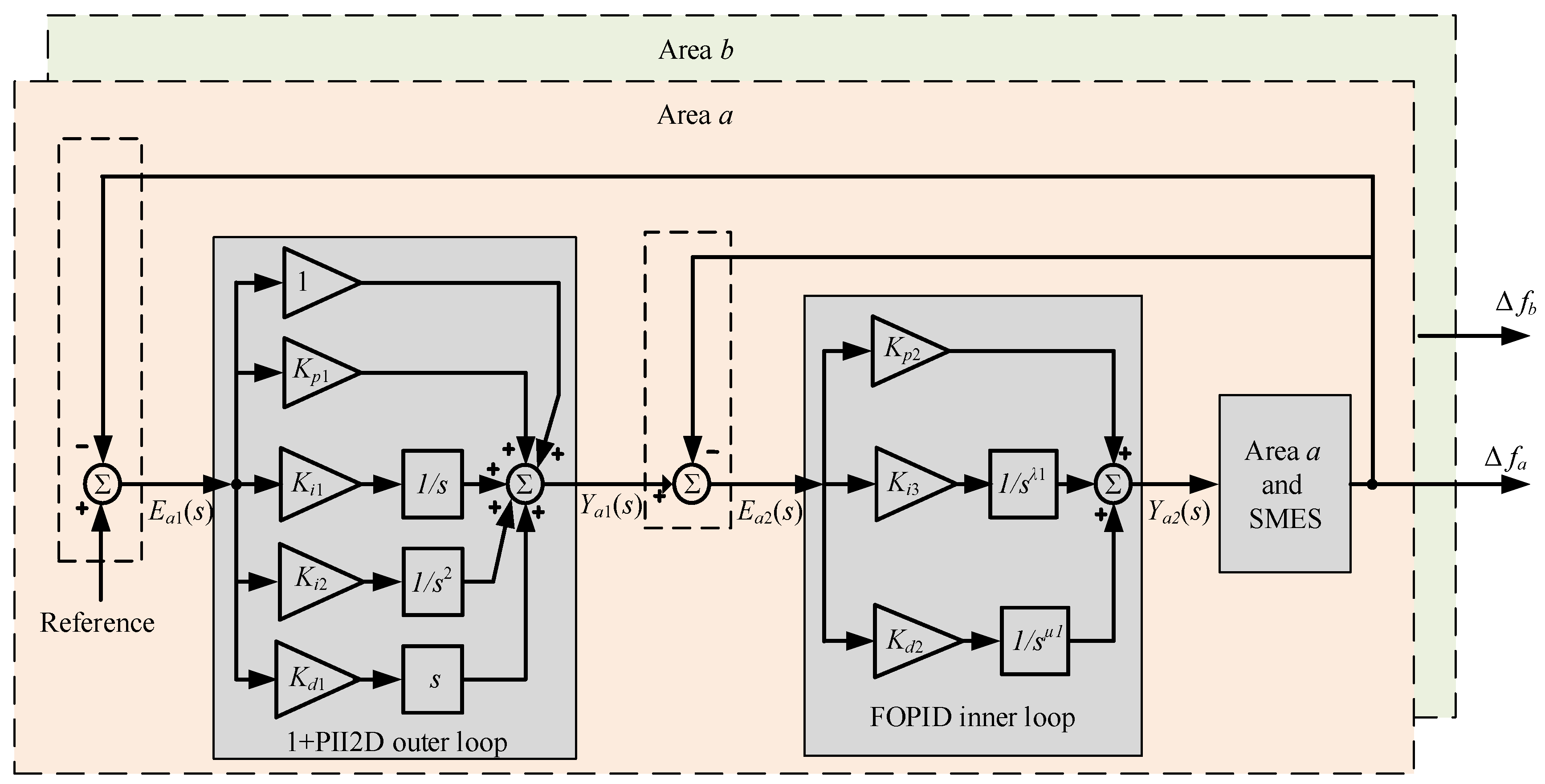
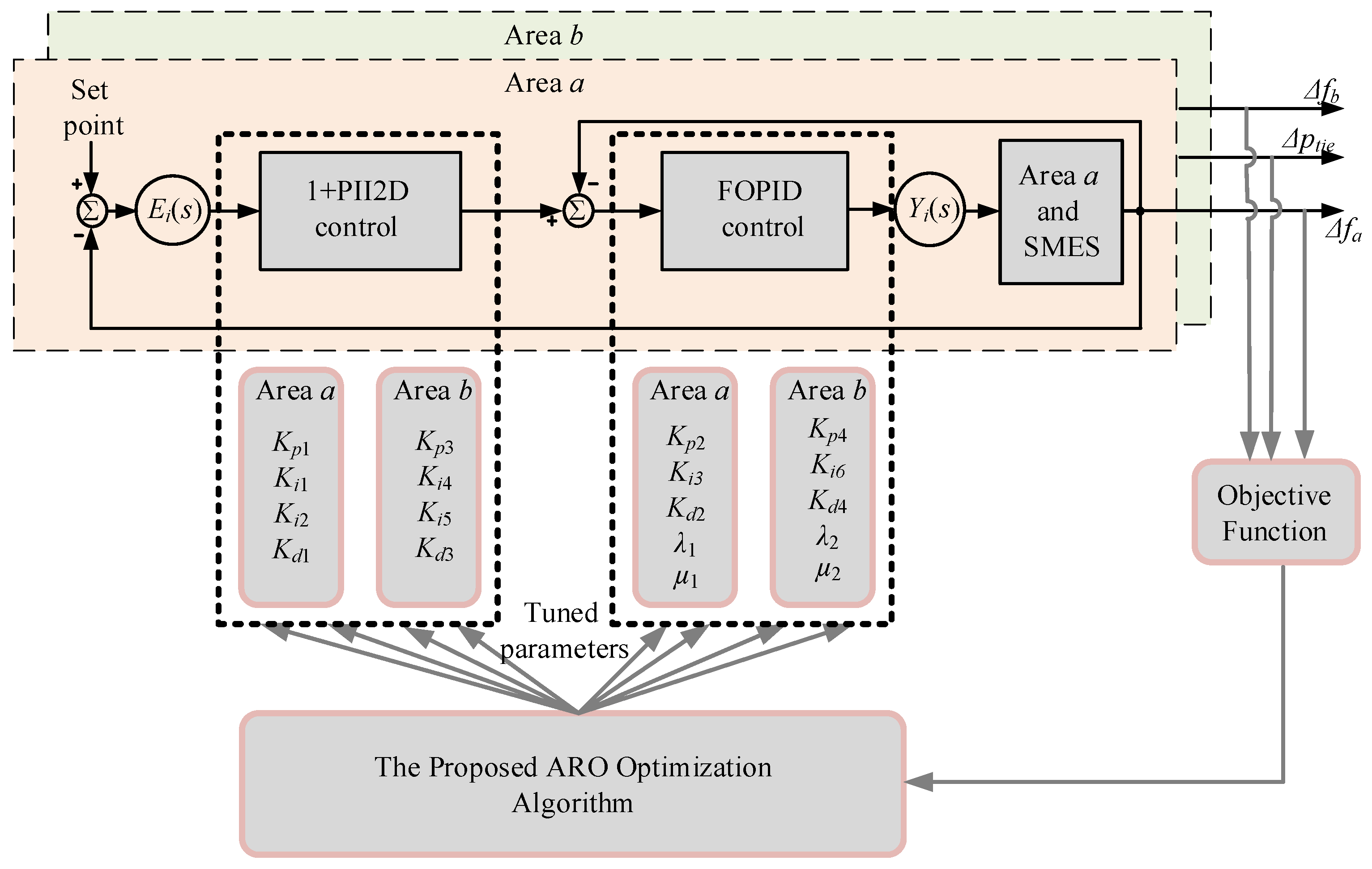
• A robust new improved hybrid controller for LFC is proposed in this paper for maintaining power grid stability and for improving frequency response behavior. The proposed LFC is constructed through using the one plus proportional integral double-integral derivative (1+PII2D) cascaded with fractional order proportional-integral-derivative (FOPID), namely, the proposed 1+PII2D/FOPID controller.
• The proposed cascaded 1+PII2D/FOPID has two loops; the outer loop uses area control errors (ACE) to mitigate slow disturbances in each area, whereas the inner loop uses a frequency measurement signal to damp fast frequency fluctuations in each area. Therefore, the proposed cascaded 1+PII2D/FOPID provides enhanced rejection possibility of disturbances.
• Application of recently presented powerful artificial rabbits optimizers (ARO) algorithm for designing the proposed cascaded 1+PII2D/FOPID LFC method. The ARO optimizer finds all the tunable parameters in a simultaneous manner for guaranteeing the best frequency response behavior in all areas.
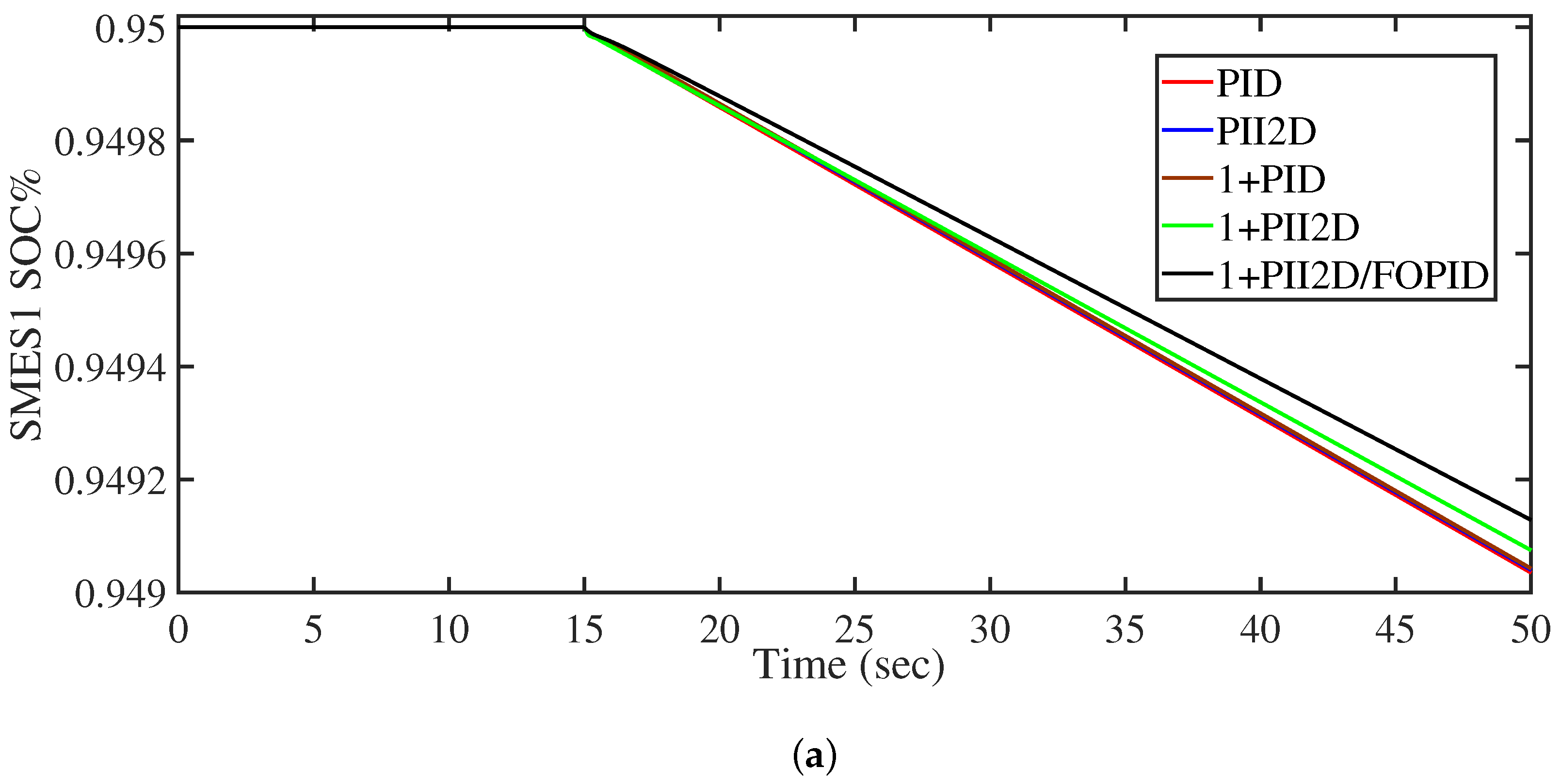
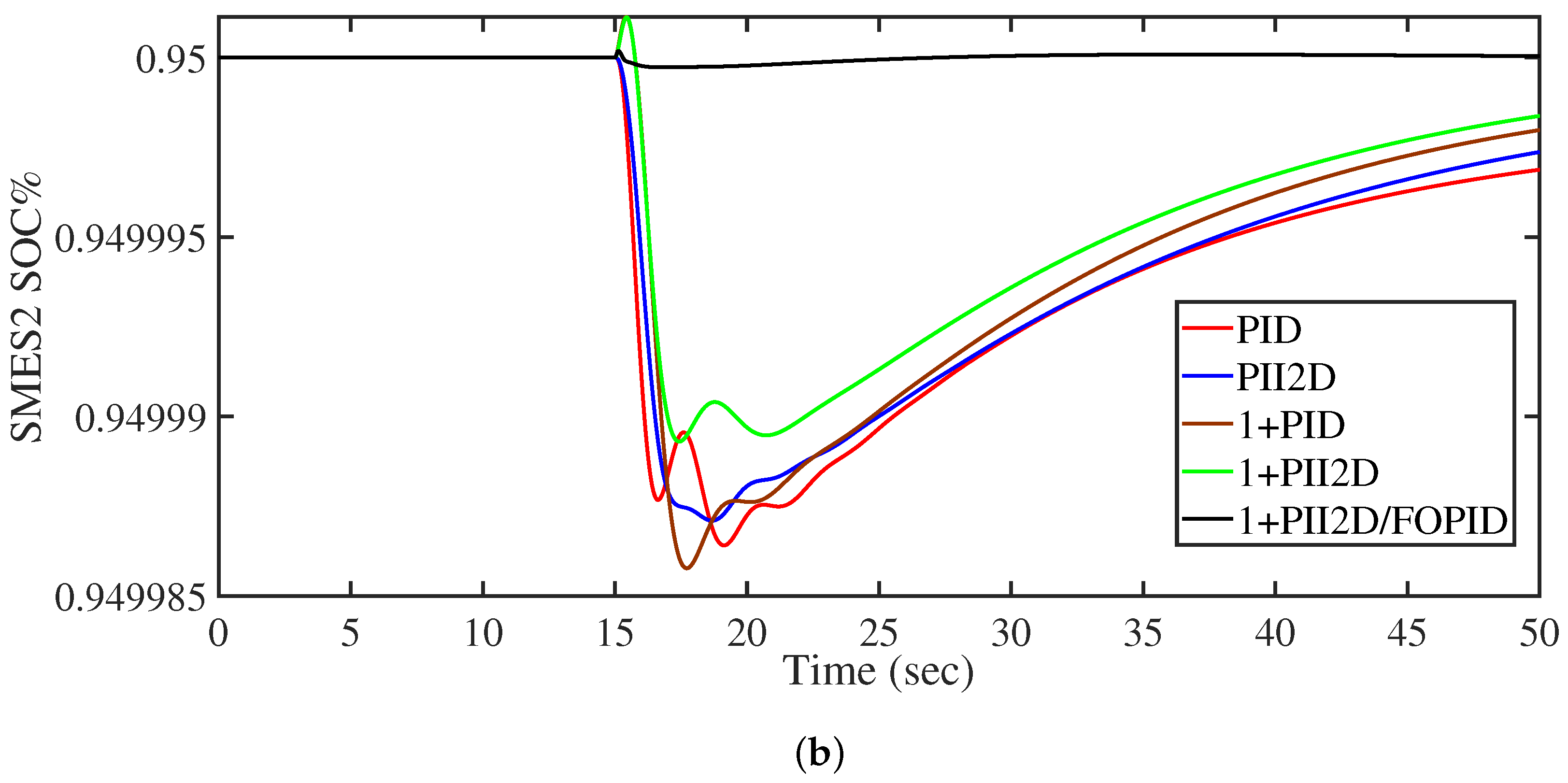
• The effects of employing SMES and their contribution in regulating grid frequency response are studied and discussed in this paper. The behavior of real wind and PV profiles jointly with different domestic and industrial load profiles are considered in this paper.

The remaining parts of this paper are organized as follows: Section 2 highlights the employed mathematical models of existing elements in the studied two areas’ interconnected power grids. Section 3 provides an overview of frequency regulation controllers in the literature and implementation of FO control. The proposed controller, the ARO principle, and proposed optimization problem are detailed in Section 4. Obtained results and their associated comparisons and description are provided in Section 5. The paper is concluded in Section 6.

2. Mathematical Description of Power Grid Elements

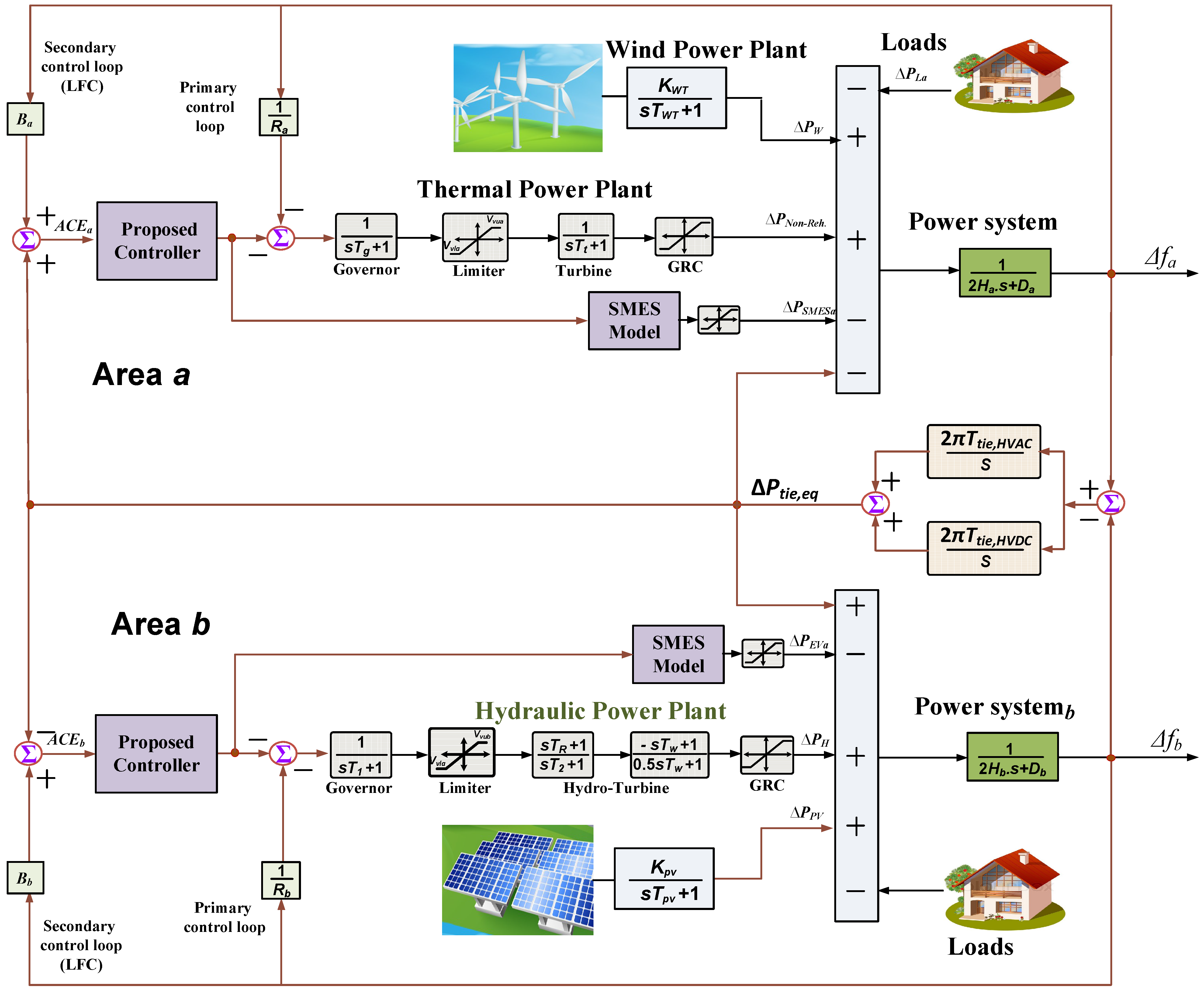
2.1. Power Grid Description

Modern power grids are basically sectionalized into multiple interconnected power grids. Each area can include conventional, renewable, storage, and different loads. The increased energy demand has made the interconnection of neighboring grids via high voltage AC transmission (HVAC) and high voltage DC transmission (HVDC) necessary to increase system capacity and reliability (the use of hybrid HVDC/HVAC transmission). The hybrid HVDC/HVAC interconnection between areas is important for economical, reliability, and fault tolerance during failures. Preserving stability between interconnected power grids faces several issues and challenges due to expected large disturbances, which may quickly propagate in the complete system. This also may cause cascaded tripping of connected units during the loss of the system’s stability. Additionally, recent additions of RESs in modern grids exhibit additional limitations due to increased penetrations of renewables. Therefore, this work presents an improved LFC method that is optimally designed to regulate the frequency response of interconnected power grids.

The two-area interconnected power grids are considered in this work as shown in the complete model representation in Figure 1. The studied system’s parameters are shown in Table 2 [50]. Additionally, the table describes the symbols of each parameter employed in the system. The system has two areas (area a interconnected with area b via hybrid HVDC/HVAC). In area a, there are a thermal power plant, wind generation unit, local loads, and SMES device. In area b, there are a hydraulic power plant, PV generation, local loads, and SMES devices. Moreover, a hybrid HVDC/HVAC line exists among the two areas for interchanging power in parallel form. There are two different controllers in the studied two-area power grid system. The LFC is responsible for controlling the power of existing generation and storage elements in each area for regulating system frequency and preserving balanced generation/loading profiles. The control and regulation done by controllers includes the sudden deviations in frequency of area a$\left(\mathrm{\Delta }{f}_a\right)$, frequency of area b$\left(\mathrm{\Delta }{f}_b\right)$, and fluctuations of tie-line power among connected areas $\left(\mathrm{\Delta }{P}_{tie,eq}\right)$. The tie-line power $\left(\mathrm{\Delta }{P}_{tie,eq}\right)$ includes the HVAC portion $\left(\mathrm{\Delta }{P}_{tie,AC}\right)$ and HVDC portion $\left(\mathrm{\Delta }{P}_{tie,DC}\right)$. Simultaneous cooperative design and parameter optimization are necessary for finding the best frequency response of power grids.

Figure 1. Complete representation model of studied power grid system.

Table 2. Power grids’ elements and parameters of considered system ($x\in \{a,b\}$) [50].

Parameters	Symbols	Values
		Area $\mathit{a}$	Area $\mathit{b}$
Capacity ratings	$P_{rx}$ (MW)	1200	1200
Droop constants	$R_x$ (Hz/MW)	2.4	2.4
Frequency bias values	$B_x$ (MW/Hz)	0.4249	0.4249
Minimum valve gates limit	$V_{vlx}$ (p.u.MW)	−0.5	−0.5
Maximum valve gates limit	$V_{vux}$ (p.u.MW)	0.5	0.5
Time constants of thermal governors	$T_g$ (s)	0.08	-
Time constants of thermal turbines	$T_t$ (s)	0.3	-
Time constants of hydraulic governors	$T_1$ (s)	-	41.6
TC of transient droop (hydraulic)	$T_2$ (s)	-	0.513
Reset times of hydraulic governors	$T_R$ (s)	-	5
Water starting times of hydro turbines	$T_w$ (s)	-	1
Power systems’ inertia constants	$H_x$ (p.u.s)	0.0833	0.0833
Power systems’ damping coefficients	$D_x$ (p.u./Hz)	0.00833	0.00833
Time constants of PV	$T_{PV}$ (s)	-	1.3
Gains of PV	$K_{PV}$ (s)	-	1
Time constants of wind	$T_{WT}$ (s)	1.5	-
Gains of wind	$K_{WT}$ (s)	1	-
Time constants of SMES converters	$T_{DCx}$ (s)	0.03	0.03
Coils of SMES	$L_x$ (H)	0.03	0.03
SMES gains	$K_{SMESx}$ (kV/unit MW)	100	100
SMES Controller gains	$K_{Idx}$ (kV/kA)	0.2	0.2
Inductor rated currents of SMES	$I_{d0x}$ (kA)	4.5	4.5
Capacity ratios of two-area systems	$A_{ab}$	−1
HVDC coefficients	$T_{tie,dc}$ (s)	0.1732
HVAC coefficients	$T_{tie,ac}$ (s)	0.0865

2.2. Dynamic Models for Generation Units

There are two conventional generation units (thermal and hydraulic) and two renewables (PV and wind). The transfer function (TF) for the thermal plant includes turbine’s TF $G_t\left(s\right)$ and governor’s TF $G_g\left(s\right)$. They are expressed as:

$$G_g\left(s\right)=\frac{1}{T_{g}s+1}$$

(1)

$$G_t\left(s\right)=\frac{1}{T_{t}s+1}$$

(2)

The TF for hydraulic plant has the speed governor, the droop compensation, and penstock turbine. The complete TF $G_h\left(s\right)$ is expressed as:

$$G_h\left(s\right)=\frac{1}{T_{1}s+1}.\frac{T_{R}s+1}{T_{2}s+1}.\frac{-T_{w}s+1}{0.5T_{w}s+1}$$

(3)

Whereas the TF model for power grids $G_{px}\left(s\right)$ is expressed as:

$$G_{px}\left(s\right)=\frac{1}{2H_{x}s+D_x}$$

(4)

A first-order TF is employed for wind units $G_{WT}\left(s\right)$ and PV units $G_{PV}\left(s\right)$ as follows:

$$G_{WT}\left(s\right)=\frac{K_{WT}}{T_{WT}s+1}$$

(5)

$$G_{PV}\left(s\right)=\frac{K_{PV}}{T_{PV}s+1}$$

(6)

2.3. SMES Modelling

SMES devices are characterized by faster response, long operating lifetime, and higher efficiency compared with other ESSs. The SMES can respond to fast disturbances in power grids, which leads to better regulation of frequency response. For connecting a SMES coil with power grids, a bidirectional DC/DC power electronic converter, DC/AC inverter, and low frequency transformer are needed [51]. The complete system is shown in Figure 2. In a normal operation scenario, the SMES is charged and it works to supply/store electrical energy to the power grids, whereas during disturbances, it helps compensate the associated fluctuations in power grids. Thence, SMES can help preserve generation/load balance. A first-order SMES model is employed in this work as shown in Figure 2. Frequency deviations of the two areas $\mathrm{\Delta }{f}_a$ and $\mathrm{\Delta }{f}_b$ with the hybrid HVDC/HVAC line and power participation of SMES $\mathrm{\Delta }{P}_{SME{S}_a}$ in area a and $\mathrm{\Delta }{P}_{SME{S}_b}$ in area b and renewables can be expressed as [51]:

$$\begin{array}{c}\mathrm{\Delta }{f}_a=\frac{1}{2H_{a}s+D_a}[\mathrm{\Delta }{P}_{Non,Reh}+\mathrm{\Delta }{P}_W-\mathrm{\Delta }{P}_{La}-\mathrm{\Delta }{P}_{SME{S}_a}-\mathrm{\Delta }{P}_{tie,eq}]\hfill \end{array}$$

(7)

$$\begin{array}{c}\mathrm{\Delta }{f}_b=\frac{1}{2H_{b}s+D_b}[\mathrm{\Delta }{P}_H+\mathrm{\Delta }{P}_{PV}-\mathrm{\Delta }{P}_{Lb}-\mathrm{\Delta }{P}_{SME{S}_b}-A_{ab}\mathrm{\Delta }{P}_{tie,eq}]\hfill \end{array}$$

(8)

whereas $\mathrm{\Delta }{P}_{tie,eq}$ stands for total tie-lines power flowing in HVDC and HVAC lines between areas. It is fully represented in the following subsection.

Figure 2. SMES power conditioning system and model for frequency regulation.

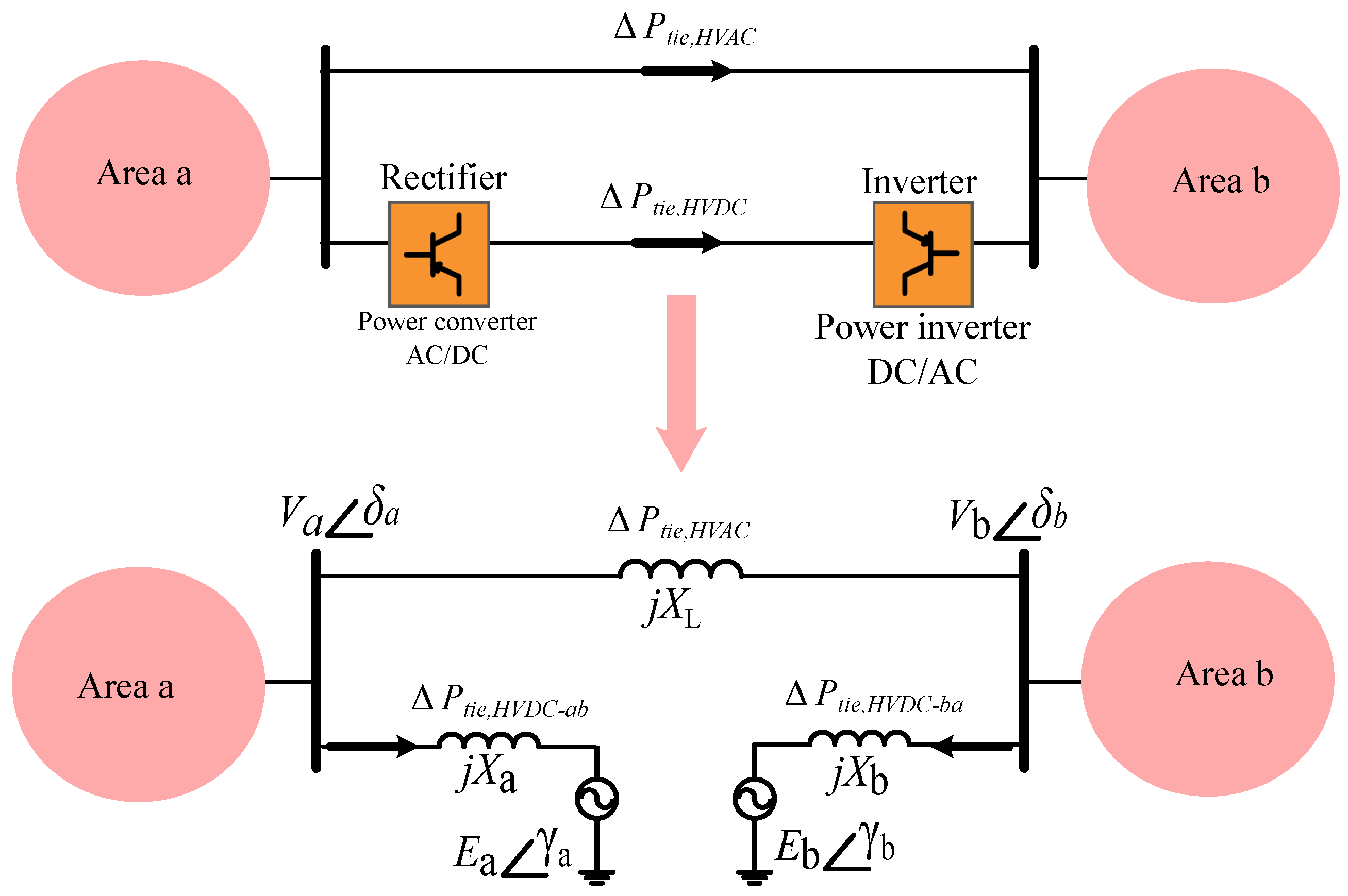
2.4. Hybrid HVDC/HVAC Line Model

Figure 3 shows the hybrid HVDC/HVAC transmission lines between the two areas and its equivalent model. The HVDC line can be split into a two-series voltage source converter/inverter system. The two converters have voltage amplitudes of $E_a$, $E_b$ and the associated angles are ${\gamma }_a$, ${\gamma }_b$, respectively. Representation of the HVDC line is made through using two impedance-based on phase reactors $X_a$, $X_b$ in each HVDC side. The power transferred from area a into area b is expressed as [51]:

$$P_{tie,D{C}_{-}ab}=\frac{V_a\ast E_a}{X_a}sin({\delta }_a-{\gamma }_a)$$

(9)

where $P_{tie,D{C}_{-}ab}$ stands for the power transferred from area a into area b through HVDC line. By linearizing the model in (9), the following expression is obtained:

$$\mathrm{\Delta }{P}_{tie,D{C}_{-}ab}=T_{tie,D{C}_{-}ab}(\mathrm{\Delta }{\delta }_a-\mathrm{\Delta }{\gamma }_a)$$

(10)

where $T_{tie,D{C}_{-}ab}$ stands for synchronizing coefficient of AC/DC power converter. It is expressed as [52]:

$$T_{tie,D{C}_{-}ab}=\frac{V_a\ast E_a}{X_a}cos({\delta }_a^0-{\gamma }_a^0)$$

(11)

Figure 3. Hybrid HVDC/HVAC model and structure.

For area b, $P_{tie,D{C}_{-}ba}$ stands for the power transferred from area b into area a through HVDC line. The power $\mathrm{\Delta }{P}_{tie,D{C}_{-}ba}$ is obtained as [51]:

$$\mathrm{\Delta }{P}_{tie,D{C}_{-}ba}=T_{tie,D{C}_{-}ba}(\mathrm{\Delta }{\delta }_b-\mathrm{\Delta }{\gamma }_b)$$

(12)

where $T_{tie,D{C}_{-}ba}$ stands for synchronizing coefficient the DC/AC power converter. It is represented as:

$$T_{tie,D{C}_{-}ba}=\frac{V_b\ast E_b}{X_b}cos({\delta }_b^0-{\gamma }_b^0)$$

(13)

In case of load/generation changes, (10) and (12) represent the tie-line power deviations of HVDC line. The power between areas (with ignoring line power loss) is expressed as [52]:

$$\mathrm{\Delta }{P}_{tie,D{C}_{-}ab}=-\mathrm{\Delta }{P}_{tie,D{C}_{-}ba}$$

(14)

Substituting (14) in (10) and (12), we obtain:

$$T_{tie,D{C}_{-}ab}(\mathrm{\Delta }{\delta }_a-\mathrm{\Delta }{\gamma }_a)=-T_{tie,D{C}_{-}ba}(\mathrm{\Delta }{\delta }_b-\mathrm{\Delta }{\gamma }_b)$$

(15)

With equal power transfer in both sides, the phase angle $\mathrm{\Delta }{\gamma }_a$ of power AC/DC converter side and phase angle $\mathrm{\Delta }{\gamma }_b$ of power DC/AC inverter side has to be as:

$$\mathrm{\Delta }{\gamma }_a=\mathrm{\Delta }{\gamma }_b=\mathrm{\Delta }\gamma$$

(16)

In (15), we can see the equal power transfer between the two sides ignoring the losses of the lines. With considering the relation in (16) and substituting it in (15), we can deduce the following:

$$\mathrm{\Delta }\gamma =\frac{\mathrm{\Delta }{\delta }_a+\left(\frac{T_{tie,D{C}_{-}ba}}{T_{tie,D{C}_{-}ab}}\right)\mathrm{\Delta }{\delta }_b}{1+\frac{T_{tie,D{C}_{-}ba}}{T_{tie,D{C}_{-}ab}}}$$

(17)

While substituting (16) into (10) gives:

$$\mathrm{\Delta }{P}_{tie,D{C}_{-}ab}=\frac{T_{tie,D{C}_{-}ab}{T}_{tie,D{C}_{-}ba}}{T_{tie,D{C}_{-}ab}+T_{tie,D{C}_{-}ba}}(\mathrm{\Delta }{\delta }_a-\mathrm{\Delta }{\delta }_b)$$

(18)

where $T_{tie,D{C}_{-}ab}$ is the synchronizing coefficient among areas a and b. Using the tie-line models in Figure 1, $\mathrm{\Delta }{P}_{tie,D{C}_{-}ab}$ is directly proportional to the difference between frequency deviations of the interconnected areas. It is expressed as:

$$\mathrm{\Delta }{P}_{tie,D{C}_{-}ab}=2\pi T_{tie,D{C}_{-}ab}\int (\mathrm{\Delta }{f}_a-\mathrm{\Delta }{f}_b)dt$$

(19)

Using (19) and the parallel lines in Figure 1 can be expressed as:

$$\mathrm{\Delta }{P}_{tie,D{C}_{-}ab}=2\pi \frac{T_{tie,D{C}_{-}ab}{T}_{tie,A{C}_{-}ab}}{T_{tie,D{C}_{-}ab}+T_{tie,A{C}_{-}ab}}\int (\mathrm{\Delta }{f}_a-\mathrm{\Delta }{f}_b)dt$$

(20)

Afterwards, using Laplace transform in (20), we can obtain the following expression:

$$\mathrm{\Delta }{P}_{tie,D{C}_{-}ab}\left(s\right)=2\pi \frac{T_{tie,eq}}{s}(\mathrm{\Delta }{f}_a\left(s\right)-\mathrm{\Delta }{f}_b\left(s\right))$$

(21)

whereas equivalent synchronization coefficient for HVDC line is determined as:

$$T_{tie,eq}=\frac{\left(T_{tie,D{C}_{-}ab}{T}_{tie,A{C}_{-}ba}\right)}{(T_{tie,D{C}_{-}ab}+T_{tie,A{C}_{-}ba})}$$

(22)

2.5. Complete Grid System Model

Based on the presented complete model of studied grid system in Figure 1 and the presented SMES model in Figure 2 and hybrid transmission line in Figure 3, the state space linearization model can be obtained and combined for the studied grid system. A general representation for the state space complete system model is expressed as:

$$\dot{x}=Ax+B_1\omega +B_{2}u$$

(23)

$$y=Cx$$

(24)

where x, y, $\omega$ and u are vectors expressing state variables’ matrix, outputs states’ vector, disturbances’ vector, and control variables’ vector, respectively, whereas A, $B_1$, $B_2$, and C stand for parameters’ matrices representing the linearized model of the presented model in Figure 1. The matrices A, $B_1$, $B_2$, and C are obtained as:

$$A=\left[\begin{array}{cccccccccc}-\frac{D_a}{2H_a}& \frac{1}{2H_a}& 0& \frac{1}{2H_a}& 0& 0& 0& 0& 0& -\frac{1}{2H_a}\\ 0& -\frac{1}{T_t}& \frac{1}{T_t}& 0& 0& 0& 0& 0& 0& 0\\ -\frac{1}{R_a{T}_g}& 0& -\frac{1}{T_g}& 0& 0& 0& 0& 0& 0& 0\\ 0& 0& 0& -\frac{1}{T_{WT}}& 0& 0& 0& 0& 0& 0\\ 0& 0& 0& 0& -\frac{D_b}{2H_b}& \frac{1}{2H_b}& 0& 0& \frac{1}{2H_b}& \frac{1}{2H_b}\\ 0& 0& 0& 0& \frac{2T_R}{R_b{T}_1{T}_2}& -\frac{2}{T_w}& \frac{2T_2+2T_w}{T_2{T}_w}& \frac{2T_R-2T_1}{T_1{T}_2}& 0& 0\\ 0& 0& 0& 0& -\frac{T_R}{R_b{T}_1{T}_2}& 0& -\frac{1}{T_2}& \frac{T_1-T_R}{T_1{T}_2}& 0& 0\\ 0& 0& 0& 0& -\frac{1}{R_b{T}_1}& 0& 0& -\frac{1}{T_1}& 0& 0\\ 0& 0& 0& 0& 0& 0& 0& 0& -\frac{1}{T_{PV}}& 0\\ 2\pi T_{tie,eq}& 0& 0& 0& -2\pi T_{tie,eq}& 0& 0& 0& 0& 0\end{array}\right]$$

(25)

$$B_1=\left[\begin{array}{cccc}-\frac{1}{2H_a}& 0& 0& 0\\ 0& 0& 0& 0\\ 0& 0& 0& 0\\ 0& \frac{K_{WT}}{T_{WT}}& 0& 0\\ 0& 0& -\frac{1}{2H_b}& 0\\ 0& 0& 0& 0\\ 0& 0& 0& 0\\ 0& 0& 0& 0\\ 0& 0& 0& \frac{K_{PV}}{T_{PV}}\\ 0& 0& 0& 0\end{array}\right],\mathrm{and}{B}_2=\left[\begin{array}{cccc}0& -\frac{1}{2H_a}& 0& 0\\ 0& 0& 0& 0\\ -\frac{1}{T_g}& 0& 0& 0\\ 0& 0& 0& 0\\ 0& 0& 0& -\frac{1}{2H_b}\\ 0& 0& \frac{2T_R}{T_1{T}_2}& 0\\ 0& 0& -\frac{T_R}{T_1{T}_2}& 0\\ 0& 0& -\frac{1}{T_1}& 0\\ 0& 0& 0& 0\\ 0& 0& 0& 0\end{array}\right]$$

(26)

$$C=\left[\begin{array}{cccccccccc}1& 0& 0& 0& 0& 0& 0& 0& 0& 0\\ B_a& 0& 0& 0& 0& 0& 0& 0& 0& 1\\ 0& 0& 0& 0& 1& 0& 0& 0& 0& 0\\ 0& 0& 0& 0& B_b& 0& 0& 0& 0& -1\end{array}\right]$$

(27)

The state variables’ matrix x can be expressed as:

$$x={\left[\begin{array}{cccccccccc}\mathrm{\Delta }{f}_a& \mathrm{\Delta }{P}_{ga}& \mathrm{\Delta }{P}_{ga1}& \mathrm{\Delta }{P}_{WT}& \mathrm{\Delta }{f}_b& \mathrm{\Delta }{P}_{gb}& \mathrm{\Delta }{P}_{gb1}& \mathrm{\Delta }{P}_{gb2}& \mathrm{\Delta }{P}_{PV}& \mathrm{\Delta }{P}_{tie,eq}\end{array}\right]}^T$$

(28)

The controlling variables vector u includes the LFC controller outputs ($AC{E}_{a}o$ and $AC{E}_{b}o$), and SMES power ($\mathrm{\Delta }{P}_{SME{S}_a}$ and $\mathrm{\Delta }{P}_{SME{S}_b}$). It is expressed as:

$$u={\left[\begin{array}{cccc}AC{E}_a& \mathrm{\Delta }{P}_{SME{S}_a}& AC{E}_b& \mathrm{\Delta }{P}_{SME{S}_b}\end{array}\right]}^T$$

(29)

Whereas the PV and wind power generation ($P_{WT}$ and $P_{PV}$) in addition to load power ($P_{la}$ and $P_{lb}$) construct disturbances’ vector $\omega$ is as follows:

$$\omega ={\left[\begin{array}{cccc}\mathrm{\Delta }{P}_{la}& P_{WT}& \mathrm{\Delta }{P}_{lb}& P_{PV}\end{array}\right]}^T$$

(30)

3. LFC Schemes in Literature and FO Operator Modeling

3.1. LFC Overview in Literature

As described in the literature review, several control schemes have been proposed for LFC using IO and FO control theories. The mostly applied IOs include I, PI, PID, PIDF, PIDD, and PIDA controllers. Their TFs are expressed as:

$$\begin{array}{c}{C}_I\left(s\right)=\frac{Y\left(s\right)}{E\left(s\right)}=\frac{K_i}{s}\\ C_{PI}\left(s\right)=\frac{Y\left(s\right)}{E\left(s\right)}=K_p+\frac{K_i}{s}\\ C_{PID}\left(s\right)=\frac{Y\left(s\right)}{E\left(s\right)}=K_p+\frac{K_i}{s}+K_{d}s\\ C_{PIDF}\left(s\right)=\frac{Y\left(s\right)}{E\left(s\right)}=K_p+\frac{K_i}{s}+K_{d}s\frac{N_f}{s+N_f}\\ C_{PIDA}\left(s\right)=\frac{Y\left(s\right)}{E\left(s\right)}=K_p+\frac{K_i}{s}+K_{d}s+K_a{s}^2\end{array}$$

(31)

Whereas FO-based LFCs TFs can be expressed as:

$$\begin{array}{c}{C}_{FOPI}\left(s\right)=\frac{Y\left(s\right)}{E\left(s\right)}=K_p+\frac{K_i}{s^{\lambda }}\\ C_{FOPID}\left(s\right)=\frac{Y\left(s\right)}{E\left(s\right)}=K_p+\frac{K_i}{s^{\lambda }}+K_d{s}^{\mu }\\ C_{FOPIDF}\left(s\right)=\frac{Y\left(s\right)}{E\left(s\right)}=K_p+\frac{K_i}{s^{\lambda }}+K_d{s}^{\mu }\frac{N_f}{s+N_f}\\ C_{TID}\left(s\right)=\frac{Y\left(s\right)}{E\left(s\right)}=K_t{s}^{-\left(\frac{1}{n}\right)}+\frac{K_i}{s}+K_{d}s\\ C_{TIDF}\left(s\right)=\frac{Y\left(s\right)}{E\left(s\right)}=K_t{s}^{-\left(\frac{1}{n}\right)}+\frac{K_i}{s}+K_{d}s\frac{N_f}{s+N_f}\\ C_{FOTID}\left(s\right)=\frac{Y\left(s\right)}{E\left(s\right)}=K_t{s}^{-\left(\frac{1}{n}\right)}+\frac{K_i}{s^{\lambda }}+K_d{s}^{\mu }\\ C_{PFOTID}\left(s\right)=\frac{Y\left(s\right)}{E\left(s\right)}=K_p+K_t{s}^{-\left(\frac{1}{n}\right)}+\frac{K_i}{s^{\lambda }}+K_d{s}^{\mu }\end{array}$$

(32)

Figure 4 summarizes some of the widely applied LFCs using IO and FO methods. The tunable control parameters are represented with colored blocks in the figure. It can be seen that FO operators increase the flexibility and number of tunable parameters compared to IO control methods.

Figure 4. Featured IOFR and FOFR for LFC in the literature (wherein tunable control parameters are shown in colored blocks): (a) PI LFC; (b) PID LFC; (c) FOPI LFC; (d) FOPID LFC; (e) PIDA; (f) TID LFC; (g) FOTID LFC; (h) PFOTID.

3.2. FO Operator Modeling

In the literature, several models exist for FO operators’ representations. FO operators can be generally expressed using $D^{\alpha }{|}_a^t$, which can take the following models [53]:

$$D^{\alpha }{|}_a^t=\left\{\begin{array}{cc}\alpha >0\to \frac{{\mathrm{d}}^{\alpha }}{\mathrm{d}{t}^{\alpha }}\hfill & \mathrm{FO}\mathrm{derivative}\hfill \\ \alpha <0\to {\int }_{t_0}^{t_{\mathrm{f}}}\mathrm{d}{t}^{\alpha }\hfill & \mathrm{FO}\mathrm{integral}\hfill \\ \alpha =0\to 1\hfill \end{array}\right.$$

(33)

In the Grunwald–Letnikov model, FO ${\alpha }^{th}$ derivative of f between a to t with h step time and $[·]$ integer operator is represented as [54]:

$$D^{\alpha }{|}_a^t=\underset{h\to 0}{lim}\frac{1}{h^{\alpha }}\sum _{r=0}^{\frac{t-a}{h}}{(-1)}^r\left(\begin{array}{c}n\\ r\end{array}\right)f(t-rh)$$

(34)

In (34), n has to be selected ($n-1$$<\alpha <n$). Binomial coefficients of the Grunwald–Letnikov model are expressed as [55]:

$$\left(\begin{array}{c}n\\ r\end{array}\right)=\frac{\mathrm{\Gamma }(n+1)}{\mathrm{\Gamma }(r+1)\mathrm{\Gamma }{(n-r+1)}^{\prime }}$$

(35)

where the gamma-function in (35) is basically expressed as:

$$\mathrm{\Gamma }(n+1)={\int }_0^{\infty }{t}^{x-1}{e}^{-t}dt$$

(36)

Whereas the Riemann–Liouville model is represented using integer values as [56]:

$$D^{\alpha }{|}_a^t=\frac{1}{\mathrm{\Gamma }(n-\alpha )}(\frac{d}{dt}{)}^n{\int }_a^t\frac{f\left(\tau \right)}{{(t-\tau )}^{\alpha -n+1}}d\tau$$

(37)

For Caputo, FO operators are expressed as:

$$D^{\alpha }{|}_a^t=\frac{1}{\mathrm{\Gamma }(n-\alpha )}{\int }_a^t\frac{f^{\left(n\right)}\left(\tau \right)}{{(t-\tau )}^{\alpha -n+1}}d\tau$$

(38)

From another side, Oustaloup-recursive approximation (ORA) for representing FO operators using integer order terms has found wide use in control theory. The ORA can be implemented easily using digital control platforms, which makes it superior over other methods. The approximate model representation for ${\alpha }^{th}$ FO derivative ($s^{\alpha }$) is made as [53,57]:

$$s^{\alpha }\approx {\omega }_h^{\alpha }\prod _{k=-N}^N\frac{s+{\omega }_k^z}{s+{\omega }_k^p}$$

(39)

where ${\omega }_k^p$ and ${\omega }_k^z$ locate poles and zeros points of the ${\omega }_h$ sequence. The poles/zeros positions are calculated as [55]:

$${\omega }_k^z={\omega }_b{\left(\frac{{\omega }_h}{{\omega }_b}\right)}^{\frac{k+N+\frac{1-\alpha }{2}}{2N+1}}$$

(40)

$${\omega }_k^p={\omega }_b{\left(\frac{{\omega }_h}{{\omega }_b}\right)}^{\frac{k+N+\frac{1+\alpha }{2}}{2N+1}}$$

(41)

$${\omega }_h^{\alpha }={\left(\frac{{\omega }_h}{{\omega }_b}\right)}^{\frac{-\alpha }{2}}\prod _{k=-N}^N\frac{{\omega }_k^p}{{\omega }_k^z}$$

(42)

In (40)–(42), there are $(2N+1)$ numbers of poles/zeros, whereas N defines ORA’s order. The ORA is preferred and selected in this work for implementing FO operators with $(M=5)$ within ($\omega \in [{\omega }_b,{\omega }_h]$) between $[{10}^{-3},{10}^3]$ rad/s.

4. Proposed 1+PII2D/FOPID Controller and ARO Algorithm

4.1. Proposed 1+PII2D/FOPID LFC

Figure 5 presents a proposed structure of LFC using the 1+PII2D/FOPID controller. Each area has a separate controller of the proposed 1+PII2D/FOPID controller. The proposed 1+PII2D/FOPID controller is a cascaded controller using outer loop using a 1+PII2D controller. The inputted signal is based on the ACE of each area. The inner loop employs the FOPID controller with the frequency deviation signal as input with the output of the outer loop. The proposed 1+PII2D/FOPID controller combines both advantages of 1+PII2D and FOPID controllers. Thence, faster frequency response, more robust control, and enhanced disturbances rejection can be achieved using proposed 1+PII2D/FOPID controller. The structure with ACE and frequency signals achieves the rejection of low frequency as well as the high frequency generation/loading disturbance. The ACE has shown ability to reject slow frequency deviations in literature, whereas the use frequency deviation loop enables rejecting fast generation/loading disturbances.

Figure 5. Proposed 1+PII2D/FOPID controller.

Based on Figure 5, the outer loops with ACE inputted signals are ($AC{E}_a$, and $AC{E}_b$) to $E_{a1}\left(s\right)$ and $E_{b1}\left(s\right)$ sides, respectively. The 1+PII2D control is proposed in this loop. The inputs to this stage are represented as:

$$\begin{array}{c}{E}_{a1}\left(s\right)=AC{E}_a=\mathrm{\Delta }{P}_{tie}+B_a\mathrm{\Delta }{f}_a\\ E_{b1}\left(s\right)=AC{E}_b=A_{ab}\mathrm{\Delta }{P}_{tie}+B_b\mathrm{\Delta }{f}_b\end{array}$$

(43)

where $\left(A_{ab}\right)$ is defined as capacity ratio between area a and area b, whereas outputted signals $Y_{a1}\left(s\right)$ and $Y_{b1}\left(s\right)$ of proposed 1+PII2D controllers are expressed as:

$$\begin{array}{c}{Y}_{a1}\left(s\right)=[1+K_{p1}+\frac{K_{i1}}{s}+\frac{K_{i2}}{s^2}+K_{d1}s].E_{a1}\left(s\right)\\ Y_{b1}\left(s\right)=[1+K_{p3}+\frac{K_{i4}}{s}+\frac{K_{i5}}{s^2}+K_{d3}s].E_{a1}\left(s\right)\end{array}$$

(44)

From (44), it is clear that each area has four tunable parameters in the outer 1+PII2D loop. In area a, the tunable parameters are ($K_{p1}$, $K_{i1}$, $K_{i2}$, and $K_{d1}$). In area b, tunable parameters include the ($K_{p3}$, $K_{i4}$, $K_{i5}$, and $K_{d3}$), Thence, a total of eight parameters are freely optimized in the outer loop with using ACE signals as inputs. In the inner loop, FOPID with added FO operators is used for implementing this stage. The inputted signals $E_{a2}\left(s\right)$ and $E_{b2}\left(s\right)$ in this stage are expressed as:

$$E_{a2}\left(s\right)=Y_{a1}\left(s\right)-\mathrm{\Delta }{f}_a{E}_{b2}\left(s\right)=Y_{b1}\left(s\right)-\mathrm{\Delta }{f}_b$$

(45)

Whereas inner loop representation using FOPID is expressed as:

$$\begin{array}{c}{Y}_{a2}\left(s\right)=[K_{p2}+\frac{K_{i3}}{s^{{\lambda }_1}}+K_{d2}{s}^{{\mu }_1}].E_{a2}\left(s\right)\\ Y_{b2}\left(s\right)=[K_{p4}+\frac{K_{i6}}{s^{{\lambda }_2}}+K_{d4}{s}^{{\mu }_2}].E_{b2}\left(s\right)\end{array}$$

(46)

From (46), each area has five tunable parameters in its inner control loop. Area a possesses the parameters ($K_{p2}$, $K_{i3}$, ${\lambda }_1$, $K_{d2}$ and ${\mu }_1$), whereas area b possesses($K_{p4}$, $K_{i6}$, ${\lambda }_2$, $K_{d4}$ and ${\mu }_2$) tunable parameters. Thence, 10 parameters are tunable in this stage.

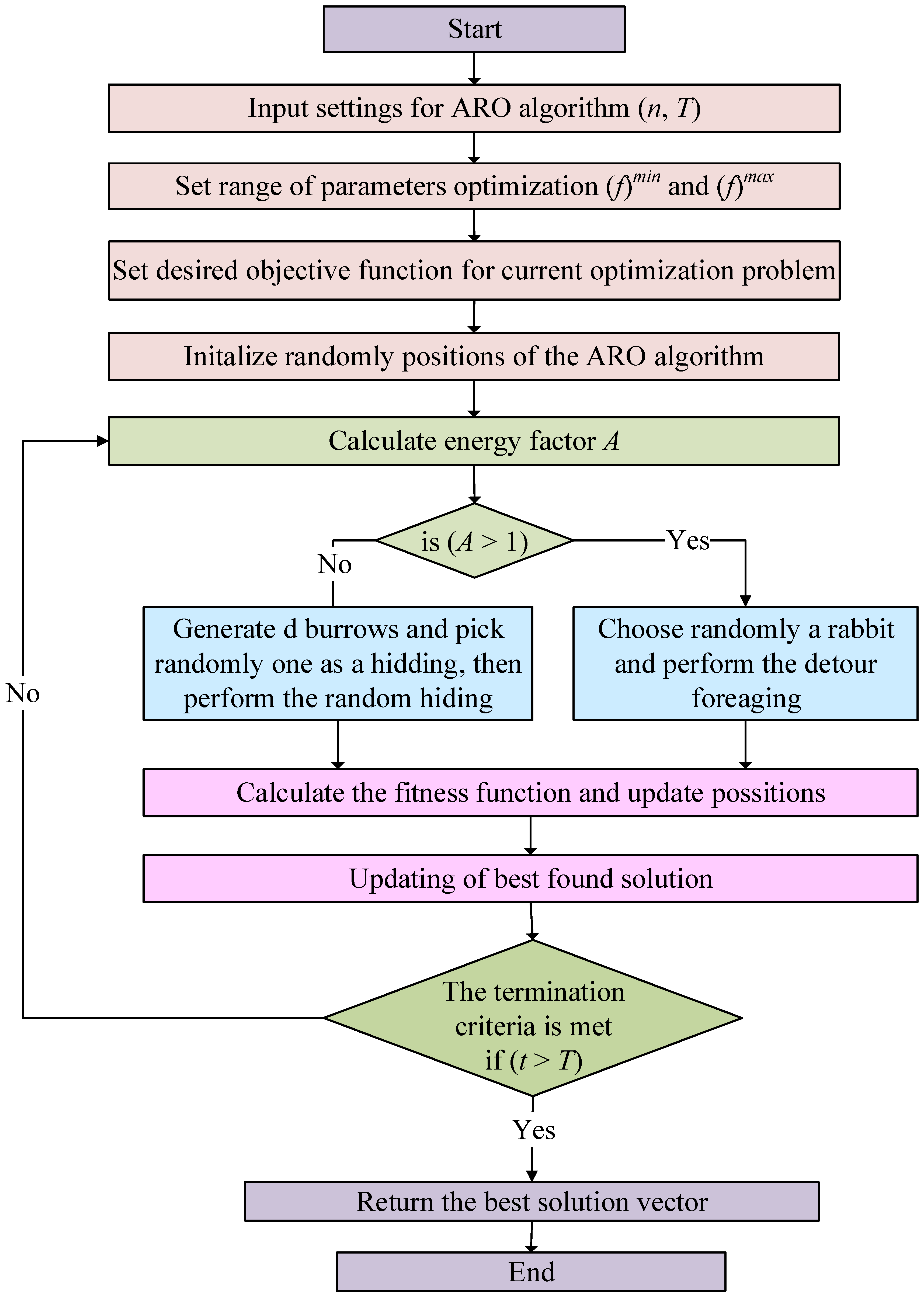
4.2. Proposed ARO Method

Recently, the artificial rabbit optimizer (ARO) has been presented in [58] based on existing tactics done by rabbits in the wild. The algorithm is inspired by the features of rabbits hunting for their meals in places distant from the own shelters and another arbitrary shelter. The ARO algorithm engages in the rummaging and hiding approach of the actual rabbits with considering their energy constrictions, which can lead to conversion amid both approaches.

• Detour Foraging: It represents the exploration stage of ARO algorithm, in which rabbits search for their food far away from their shelter. In the ARO algorithm, each rabbit is considered as having its arena and food with a number d of own holes. The rabbit can move arbitrarily to the other existing arenas for hunting food. ITs numerical prototype representation of exploration phase for each rabbit can be expressed as [58]:

  $$\begin{array}{c}{v}_i(t+1)=x_i\left(t\right)+R\times (x_i\left(t\right)-x_j\left(t\right))+round(0.5\times (0.05+r_1))\times n_1\\ i,j=1,2,...,n\mathrm{and}i\ne j\end{array}$$

  (47)

  where $v_i(t+1)$ stands for candidate locations when $i^{th}$ rabbit is at $(t+1)$ time, $x_i\left(t\right)$ stands for location of $i^{th}$ rabbit at time $\left(t\right)$, n stands for rabbits’ population size, R represents an running operator, $round$ function is rounding value at nearest integer value, $r_1$ represents random number between (0, 1), and $n_1$ is subjected to standard normal distributions. The calculation of R is performed as [59]:

  $$\begin{array}{c}R=c\times L\end{array}$$

  (48)

  where L stands for running length, whereas c stands for mapping vector. L is determined as:

  $$\begin{array}{c}L=(e-e^{{\left(\frac{t-1}{T}\right)}^2}\times sin\left(2\pi r_2\right)\hfill \end{array}$$

  (49)

  where $r_2$ stands for random number between (0,1). The value of $c\left(k\right)$ is determined as [60]:

  $$\begin{array}{c}c\left(k\right)=\left\{\begin{array}{c}1,\mathrm{if}k=g\left(l\right)\hfill \\ 0,elsewhere\hfill \end{array}\right.,\mathrm{where}k=1,...,d\mathrm{and}l=1,...,[r_3\times g\times d]\hfill \end{array}$$

  (50)

  where d stands for problem dimension, and $r_3$ stands for random number between (0, 1). Whereas the value of g is determined as [58]:

  $$\begin{array}{c}g=randperm\left(d\right),\mathrm{and}{n}_1:N(0,1)\end{array}$$

  (51)

  where $randperm$ stands for randomizing permutation of integers from 1 to d.
• Arbitrary hiding: It represents the exploitation phase of ARO algorithm. With individual repetition in ARO algorithm, rabbits constantly produce d hideaways along individual dimensions of hunting area. They continually arbitrarily select single hole from all available holes for hiding themselves to lessen likelihood being hunted. In which, the $f^{th}$ hole for $i^{th}$ rabbit is determined by [60]:

  $$\begin{array}{c}{b}_{i,j}\left(t\right)=x_i\left(t\right)+H\times g\times x_i\left(t\right)\hfill \end{array}$$

  (52)

  where H stands for hiding parameter, and i = 1, …, n and j =1, …, d. The value of H is determined as [61]:

  $$\begin{array}{c}H=\frac{T-t+1}{T}\times r_4,\mathrm{and}{n}_2:N(0,1)\end{array}$$

  (53)

  where $r_4$ stands for random number between (0, 1).

  $$\begin{array}{c}g\left(k\right)=\left\{\begin{array}{c}1,\mathrm{if}k=j\hfill \\ 0,elsewhere\hfill \end{array}\right.,\mathrm{where}k=1,...,d\hfill \end{array}$$

  (54)
  The determination of arbitrary hiding approaches is numerically expressed as [58]:

  $$\begin{array}{c}{v}_i(t+1)=x_i\left(t\right)+R\times (r_4\times b_{i,r}\left(t\right)-x_i\left(t\right)),\mathrm{and}i=1,...,n\end{array}$$

  (55)

  where $b_{i,r}\left(t\right)$ is a randomly selected burrow for hiding from its own d burrow, $r_4$ stands for random number between (0, 1). After a complete cycle of the explorations and exploitations process, the rabbit’s spot is updated through [59]:

  $$\begin{array}{c}{x}_i(t+1)=\left\{\begin{array}{c}{x}_i\left(t\right),f\left(x_i\left(t\right)\right)\le f\left(v_i(t+1)\right)\hfill \\ v_i(t+1),f\left(x_i\left(t\right)\right)>f\left(v_i(t+1)\right)\hfill \end{array}\right.\hfill \end{array}$$

  (56)
• Energy constriction: It represents the change process from the exploration to the exploitation phase. The rabbits are able to undergo exploration during the first phase, and are followed by the exploitation process during the next phase. These different searching processes are due to rabbits’ energy loss over the due course of time. The energy matter can be designed through using the following [58]:

  $$\begin{array}{c}A\left(t\right)=r\times (1-\frac{t}{T})ln\left(\frac{1}{r}\right)\end{array}$$

  (57)

The ARO optimizer flowchart is shown in Figure 6 for optimizing the proposed LFC parameters.

Figure 6. ARO algorithm for the proposed optimized controller.

4.3. Optimization of Parameters

For more robust and stable frequency response in interconnected power grids, proper selection and determinations of tunable LFC parameters are important. In the proposed 1+PII2D/FOPID controller, each area has nine tunable parameters (four in the outer loop and five in the inner loop). This leads to having 18 total of tunable parameters in the studied two-area power grids. Using ARO optimizer, the 18 parameters are simultaneously optimized and determined for achieving the best frequency response performance. Therefore, improved design process and optimized performance are achievables in the proposed optimization algorithm.

The common objectives for control tracking include the integral squared-error (ISE), the integral absolute-error (IAE), the integral time-squared-error (ITSE), and the integral time-absolute-error (ITAE) objectives. Their representation and calculations are made as:

$$\begin{array}{c}ISE=\int {\displaystyle \sum _{i=1}^m}\left(e_i^2\right)\mathrm{d}t\\ IAE=\int {\displaystyle \sum _{i=1}^m}abs\left(e_i\right)\mathrm{d}t\\ ITSE=\int {\displaystyle \sum _{i=1}^m}\left(e_i^2\right)t.\mathrm{d}t\\ ITAE=\int {\displaystyle \sum _{i=1}^m}abs\left(e_i\right)t.\mathrm{d}t\end{array}$$

(58)

It is important to highlight the main objectives to drive the optimization process in this part. The various load and generation variations are reflected as frequency deviations due to the power unbalance in each area. Thence, the designed controllers have to maintain the frequency deviations at its minimum values for more robust, stable, reliable and effective frequency regulation of each interconnected area. Additionally, the tie-line power deviations have to be preserved at its minimum values. Therefore, in the proposed optimization problem, the LFC has to regulate frequency response in each area in addition to the tie-line power of hybrid HVDC/HVAC lines. Thence, the proposed method has to minimize $\mathrm{\Delta }{f}_a$, $\mathrm{\Delta }{f}_b$, and $\left(\mathrm{\Delta }{P}_{tie,eq}\right)$, in which the objective to minimize $\left(\mathrm{\Delta }{P}_{tie,eq}\right)$ has two parts of HVDC and HVAC lines. The formulations of ISE, IAE, ITSE, and ITAE objectives are mathematically expressed as:

$$\begin{array}{c}ISE=\underset{0}{\overset{t_s}{\int }}({\left(\mathrm{\Delta }{f}_a\right)}^2+{\left(\mathrm{\Delta }{f}_b\right)}^2+{\left(\mathrm{\Delta }{P}_{tie}\right)}^2)\mathrm{d}t\\ IAE=\underset{0}{\overset{t_s}{\int }}(abs\left(\mathrm{\Delta }{f}_a\right)+abs\left(\mathrm{\Delta }{f}_b\right)+abs\left(\mathrm{\Delta }{P}_{tie}\right))\mathrm{d}t\\ ITSE=\underset{0}{\overset{t_s}{\int }}({\left(\mathrm{\Delta }{f}_a\right)}^2+{\left(\mathrm{\Delta }{f}_b\right)}^2+{\left(\mathrm{\Delta }{P}_{tie}\right)}^2).t\mathrm{d}t\\ ITAE=\underset{0}{\overset{t_s}{\int }}(abs\left(\mathrm{\Delta }{f}_a\right)+abs\left(\mathrm{\Delta }{f}_b\right)+abs\left(\mathrm{\Delta }{P}_{tie}\right)).t\mathrm{d}t\end{array}$$

(59)

The proposed ARO optimization of tunable 18 parameters is subjected to the following parameters constraints in the proposed optimization method:

$$\begin{array}{c}{K}_p^{min}\le K_{p1},K_{p2}\le K_p^{max}\\ K_i^{min}\le K_{i1},K_{i2},K_{i3}\le K_i^{max}\\ K_d^{min}\le K_{d1},K_{d2}\le K_d^{max}\\ {\lambda }^{min}\le \lambda \le {\lambda }^{max}\\ {\mu }^{min}\le \mu \le {\mu }^{max}\end{array}$$

(60)

where ${\left(f\right)}^{min}$ represents lower limiting values and ${\left(f\right)}^{max}$ represents upper limiting values of tunable parameters in the proposed ARO method. The ${\left(f\right)}^{min}$ of parameters ($K_p^{min}$, $K_i^{min}$, and $K_d^{min}$) are adjusted at zero, whereas ${\left(f\right)}^{max}$ of parameters ($K_p^{max}$, $K_i^{max}$, and $K_d^{max}$) are adjusted at 5 in proposed ARO algorithm. The ${\left(f\right)}^{min}$ of $\lambda$ and $\mu$ (${\lambda }^{min}$, and ${\mu }^{min}$, respectively) are adjusted at zero, whereas ${\left(f\right)}^{max}$ of $\lambda$ and $\mu$ (${\lambda }^{max}$, and ${\mu }^{max}$, respectively) are adjusted at 1. Figure 7 presents the complete proposed ARO-based optimization method.

Figure 7. Proposed ARO-based proposed controller design and parameters optimization.

5. Results and Discussions

The simulated case study and the studied controllers are implemented using Matlab Simulink platform linked with the m-file programming environment. The various connection/disconnection scenarios and tests are validated and compared in this paper with simulating the remote interconnected MG with two areas. Additionally, the various optimally designed controllers are tested in the same environment and conditions for the fair comparisons. The ARO optimization program and the controller objective functions are programmed using the m-file of Matlab program. The ARO algorithm is run with a maximum number of iterations of 100 iterations, while the size of the population is set at eight for ARO algorithm. The obtained optimum parameters are shown in Table 3. This part highlights the validation and efficacy of the proposed new cascaded 1+PII2D-FOPID controller and the role of the SMES device for enhancing the LFC of a dual MG system. The vigorous performance of the proposed 1+PII2D-FOPID concept is compared with conventional and advanced control techniques, such as PID, PII2D, 1+PID, and 1+PII2D under the following different operating conditions for validation.

Table 3. The optimized LFC parameters using ARO algorithm under SLC action.

Control	Area	Coefficients
		${\mathit{K}}_{\mathit{p}\mathbf{1}}$	${\mathit{K}}_{\mathit{i}\mathbf{1}}$	${\mathit{K}}_{\mathit{i}\mathbf{2}}$	${\mathit{K}}_{\mathit{d}\mathbf{1}}$	${\mathit{K}}_{\mathit{p}\mathbf{2}}$	${\mathit{K}}_{\mathit{i}\mathbf{3}}$	${\mathit{K}}_{\mathit{d}\mathbf{2}}$	$\mathit{\lambda }$	$\mathit{\mu }$
PID	Area a	2.2534	2.9881	-	3.9329	-	-	-	-	-
	Area b	2.1632	3.6812	-	0.9798	-	-	-	-	-
PII2D	Area a	3.0328	3.3456	0.9562	0.1223	-	-	-	-	-
	Area b	4.1745	3.1061	2.0038	0.0364	-	-	-	-	-
1+PID	Area a	4.4215	3.8856	-	0.3672	-	-	-	-	-
	Area b	3.6573	2.7466	-	0.0532	-	-	-	-	-
1+PII2D	Area a	4.5574	3.2037	3.7654	0.9114	-	-	-	-	-
	Area b	4.2711	3.5778	2.6247	1.0947	-	-	-	-	-
1+PII2D/FOPID	Area a	3.8719	4.4043	0.45528	4.9478	4.7938	4.7797	4.8851	0.74836	0.8521
	Area b	4.6081	4.4099	1.8515	2.8065	2.2303	3.1694	4.0063	0.6355	0.8204

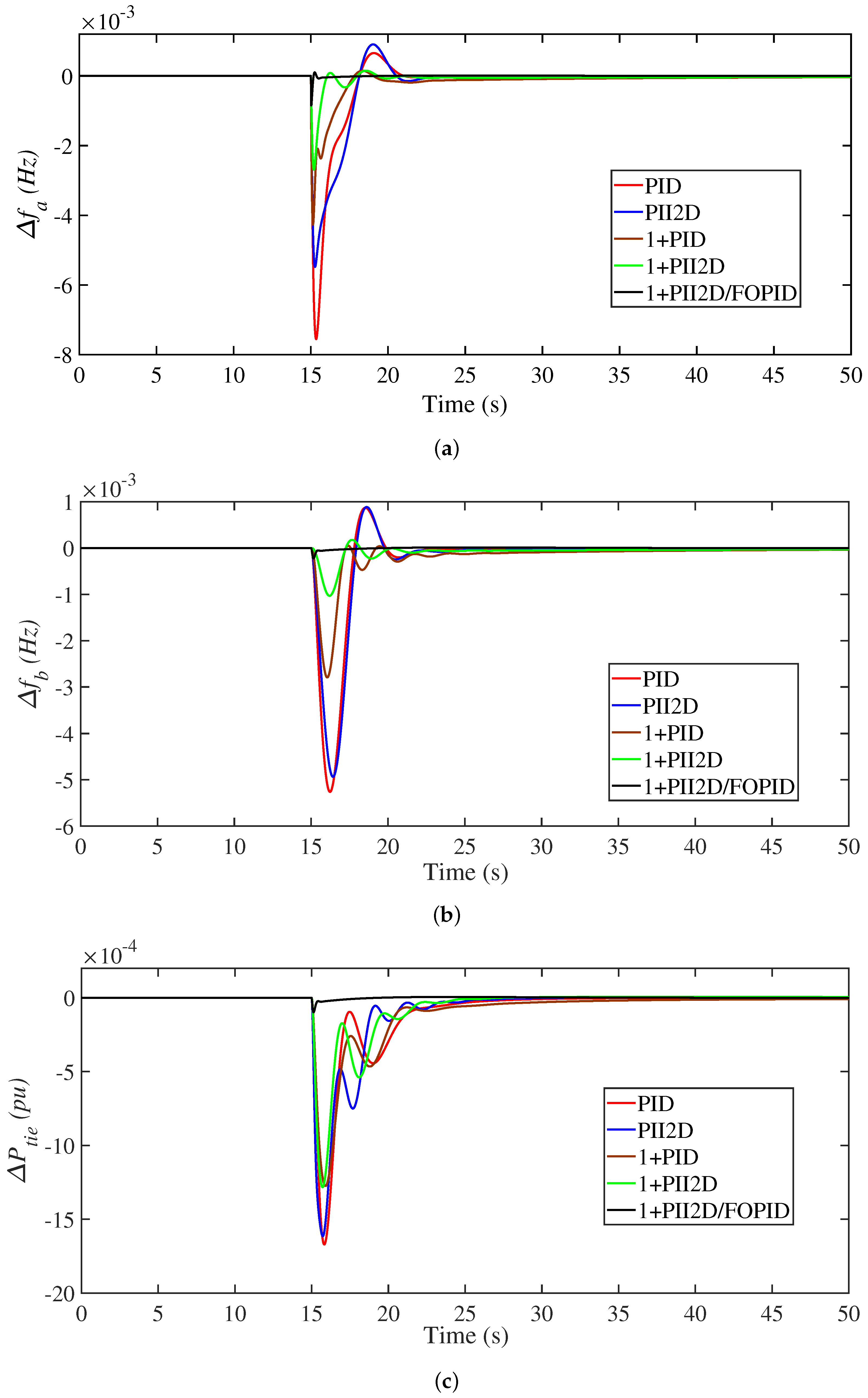
• Scenario 1: Action of step load change (SLC) with HVDC link.
• Scenario 2: Action of step load change (SLC) without HVDC link.
• Scenario 3: Action of the domestic and industrial loads.
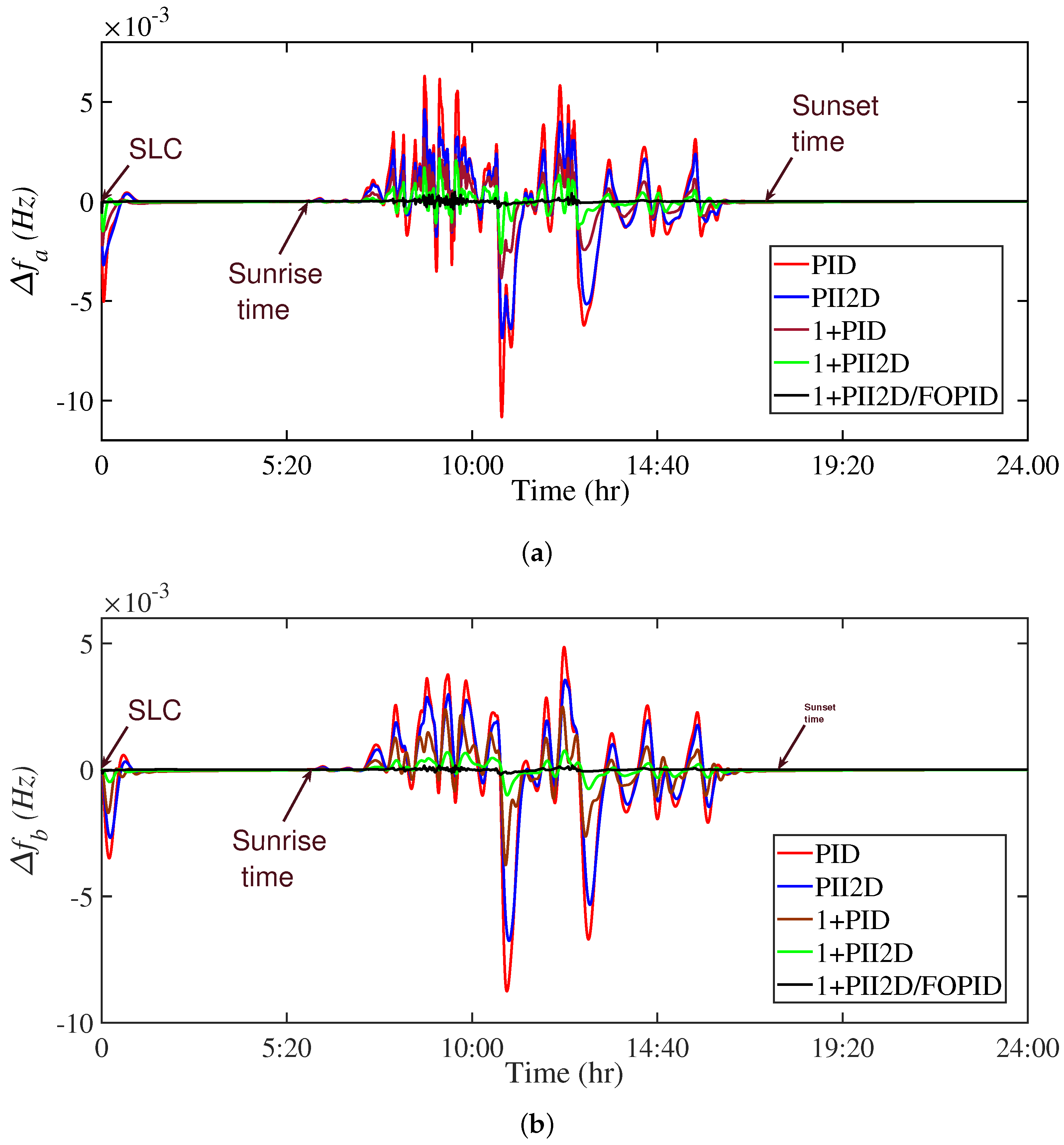
• Scenario 4: Action of the PV fluctuations.
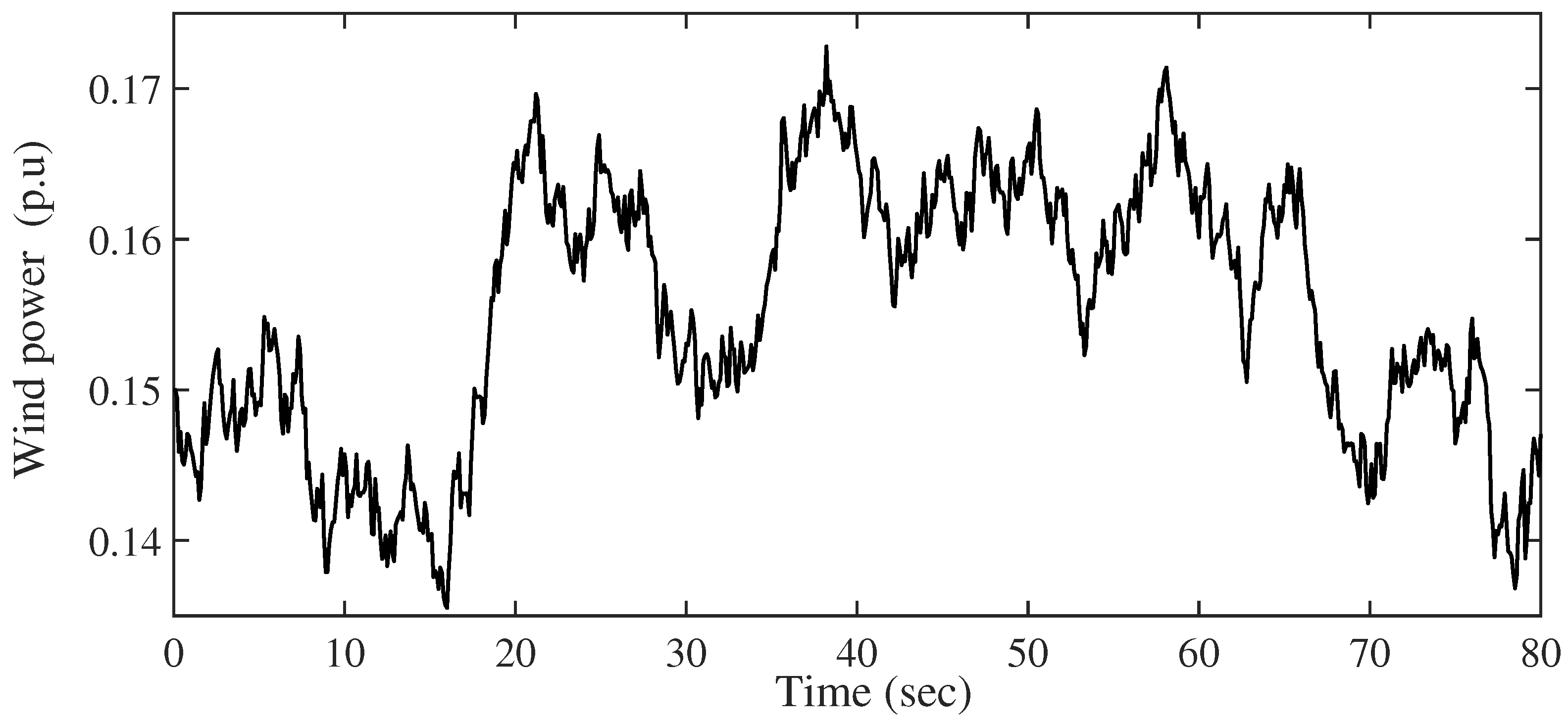
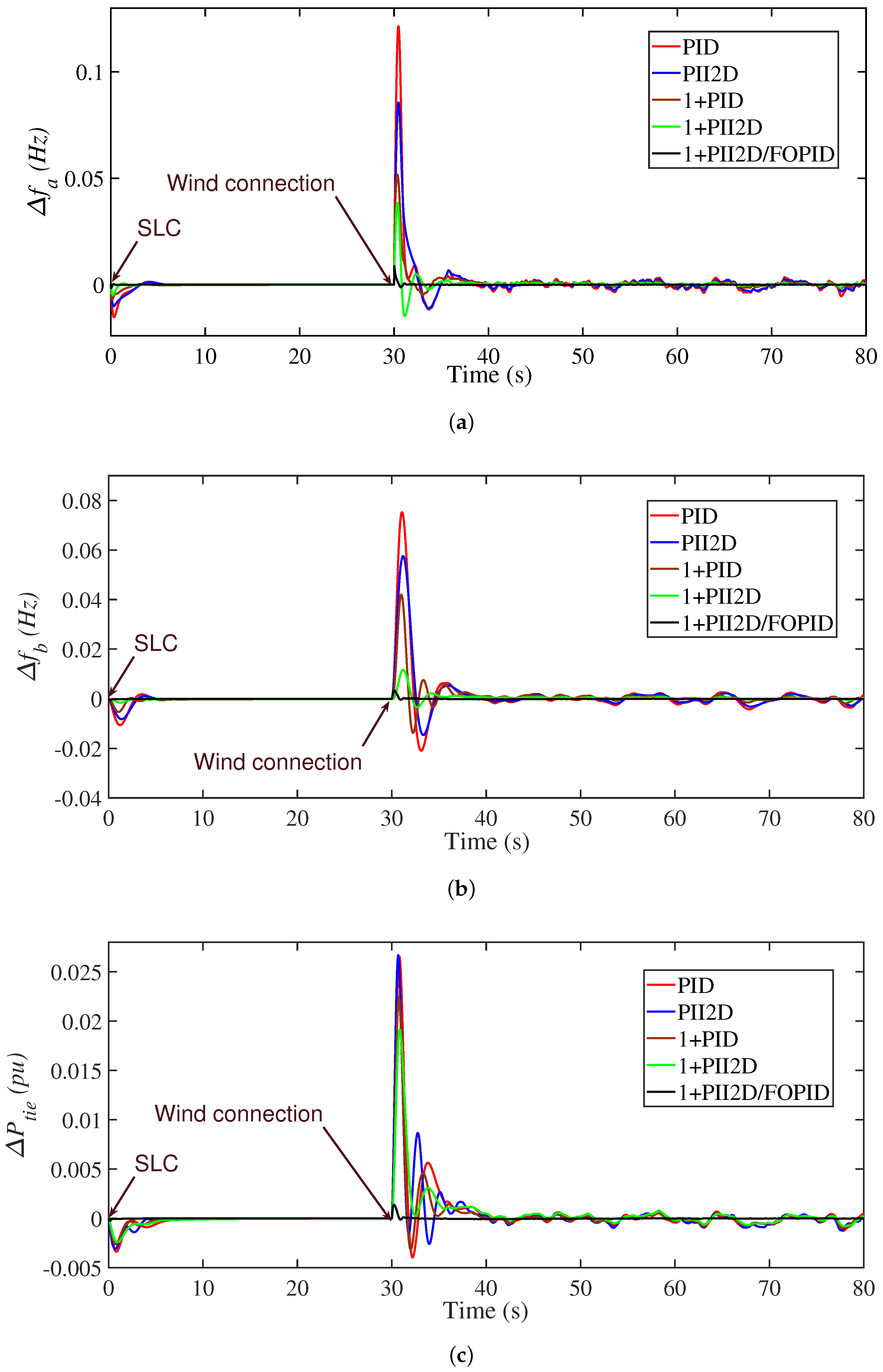
• Scenario 5: Action of wind generation fluctuations.

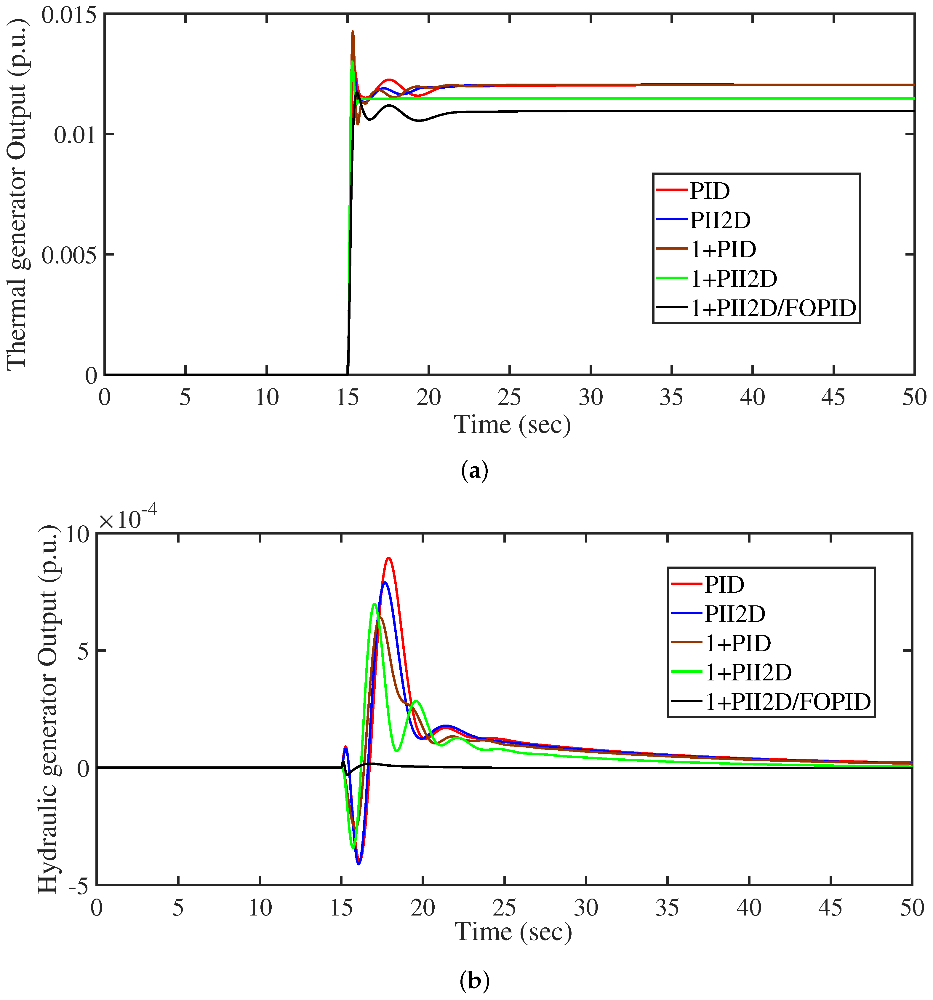
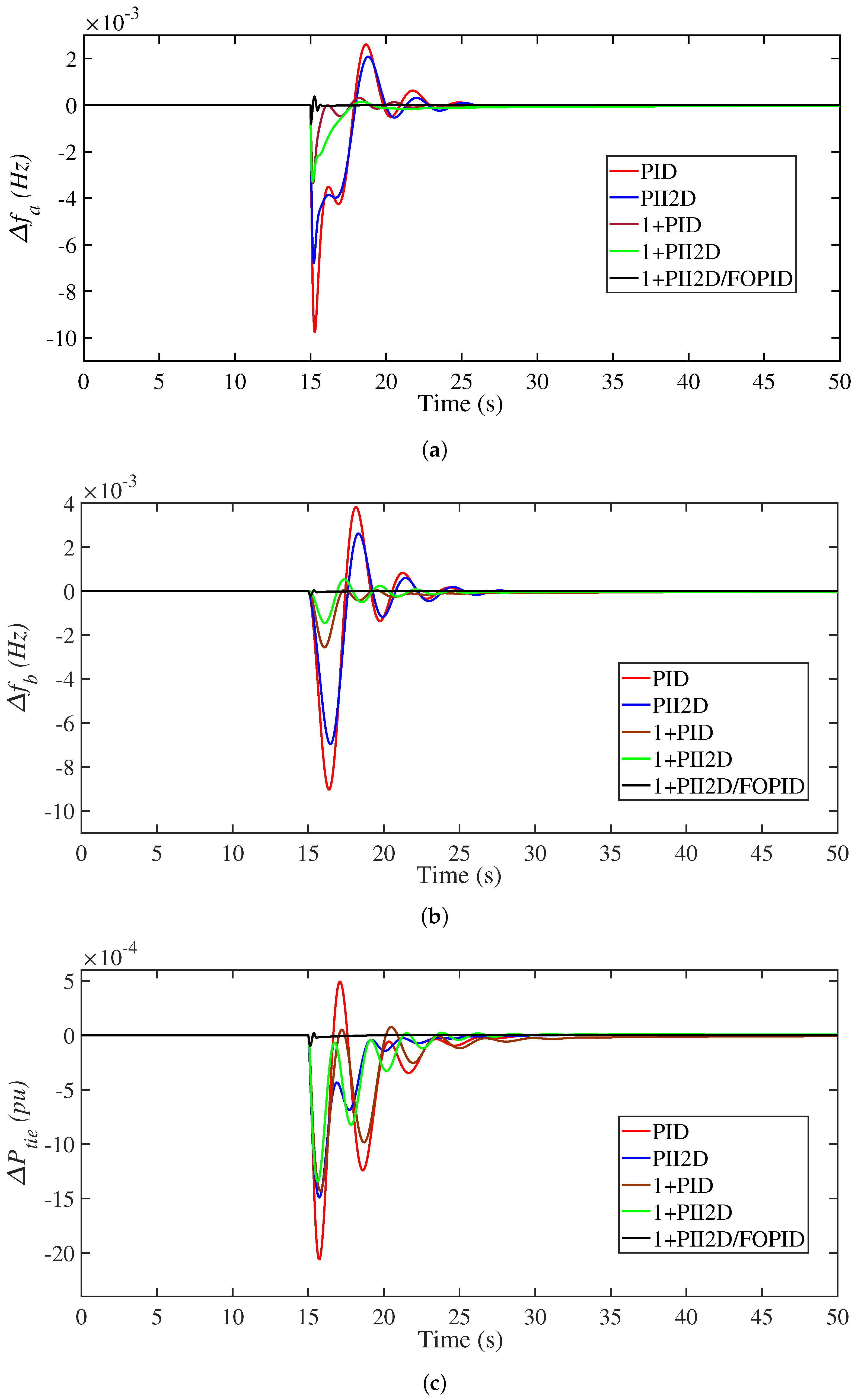
5.1. Scenario No. 1: Impact of SLC with HVDC Link

In the first scenario for testing the proposed 1+PII2D-FOPID controller for LFC and SMES system on the studied dual area system in Figure 1, 1.5% SLC is stratified in area a at t = 15 s. The multi-area system frequency and power deviations response for the proposed techniques at SLC is compared to PID, PII2D, 1+PID, and 1+PII2D controllers as shown in Figure 8. It is inferred from this figure that the conventional PID controller performs the least well among the other techniques in terms of high undershoot value at 0.0076 Hz in area a and 0.0053 Hz in area b and 0.0017 p.u. for tie-line power. Meanwhile, the PII2D keeps the frequency deviations at 0.0055 in area a and 0.0049 Hz in area b with 0.0016 p.u in exchange power. The 1+PID and 1+PII2D controllers offered positive outcomes in comparison to earlier controllers by damping the deviations to acceptable levels. However, the 1+PII2D/FOPID control has the superiority in regulating the frequency and power deviations very quickly and with less oscillations than other controllers. In addition, Table 4 provides further comparisons between the suggested controller and other state-of-the-art control techniques. It can be noted in this table that the proposed 1+PII2D/FOPID approach has the smallest maximum overshoot (MO), undershoot (MU) and settling time (ST) for two-area frequencies and exchange tie-line power. On the other hand, the control signal from the proposed cascaded 1+PII2D/FOPID controller can obtain the fast SMES performance and more SMES discharge as well as the lower power from the conventional thermal and hydraulic generators than the other controllers as shown in Figure 9, Figure 10 and Figure 11, respectively. Therefore, it is noticeable from the illustrated results that the proposed cascaded 1+PII2D/FOPID controller based on the new ARO technique is the most robust one in that scenario for LFC.

Figure 8. Obtained results at Scenario 1. (a) $\mathrm{\Delta }{f}_a$; (b) $\mathrm{\Delta }{f}_b$; (c) $\mathrm{\Delta }{P}_{tie}$.

Table 4. Performance measurements for the tested scenarios.

Scn.	Controller	$\mathrm{\Delta }{\mathit{f}}_{\mathit{a}}$			$\mathrm{\Delta }{\mathit{f}}_{\mathit{b}}$			$\mathrm{\Delta }{\mathit{P}}_{\mathit{tie}}$
		MO	MU	ST	MO	MU	ST	MO	MU	ST
No. 1	PID	0.0007	0.0076	14	0.0008	0.0053	20	0.00009	0.0017	27
	PII2D	0.00009	0.0055	14	0.00008	0.0049	19	0.00002	0.0016	25
	1+PID	0.00015	0.0043	35	0.00005	0.0028	37	0.00006	0.0013	32
	1+PII2D	0.00008	0.0027	29	0.00017	0.0011	31	0.00009	0.0012	25
	1+PII2D/FOPID	0.00006	0.00085	7	0	0.00018	9	0	0.000005	7
No. 2	PID	0.0026	0.0098	18	0.0038	0.0091	19	0.0005	0.0021	16
	PII2D	0.0021	0.0067	17	0.0026	0.0069	15	0.00004	0.0015	14
	1+PID	0.00031	0.0035	23	0.00006	0.0026	18	0.00007	0.0014	24
	1+PII2D	0.00015	0.0031	27	0.00052	0.0015	22	0.00001	0.0013	20
	1+PII2D/FOPID	0.00003	0.00079	10	0	0.0002	9	0	0.00009	8
No. 3	PID	0.0695	0.1174	23	0.0419	0.0734	19	0.0145	0.0258	18
	PII2D	0.0688	0.0821	20	0.0139	0.0565	18	0.0034	0.0252	21
	1+PID	0.0299	0.0501	18	0.0121	0.0408	17	0.0024	0.0216	16
	1+PII2D	0.0216	0.0363	16	0.0029	0.0115	15	0.0103	0.0185	14
	1+PII2D/FOPID	0.0011	0.0085	8	0.0002	0.0032	9	0.0073	0.0007	6
No. 4	PID	0.0063	0.0108	HS	0.0048	0.0088	HS	0.0017	0.0026	HS
	PII2D	0.0046	0.0068	HS	0.0036	0.0067	HS	0.0015	0.0022	HS
	1+PID	0.0031	0.0037	MS	0.0025	0.0038	MS	0.0012	0.0018	MS
	1+PII2D	0.0021	0.0026	MS	0.0007	0.0009	MS	0.0011	0.0017	MS
	1+PII2D/FOPID	0.0004	0.0003	LS	0.00009	0.0003	LS	0.00006	0.00008	LS
No. 5	PID	0.1211	0.0117	HS	0.0751	0.0209	HS	0.0267	0.0038	HS
	PII2D	0.0845	0.0112	HS	0.0575	0.0142	HS	0.0263	0.0026	HS
	1+PID	0.0513	0.0046	MS	0.0419	0.0134	MS	0.0223	0.0029	MS
	1+PII2D	0.0379	0.0145	MS	0.0113	0.0031	MS	0.0191	0.0028	MS
	1+PII2D/FOPID	0.0076	0.0012	LS	0.0031	0.0003	LS	0.0013	0.0001	LS

HS = High oscillation, MS = Medium oscillation, LS = Low oscillation.

Figure 9. SMES performance at Scenario 1. (a) $\mathrm{\Delta }{P}_{SME{S}_a}$; (b) $\mathrm{\Delta }{P}_{SME{S}_b}$.

Figure 10. SMES SOC at Scenario 1. (a) $\mathrm{\Delta }SO{C}_{SME{S}_a}$; (b) $\mathrm{\Delta }SO{C}_{SME{S}_b}$.

Figure 11. Generators’ output at Scenario 1. (a) $\mathrm{\Delta }{P}_{Non,Reh}$; (b) $\mathrm{\Delta }{P}_H$.

5.2. Scenario No. 2: Impact of SLC without HVDC Link

The capability of the proposed coordination between the novel cascaded 1+PII2D/FOPID controller based on the ARO technique is tested under a dangerous scenario which may occur when the HVDC link is disconnected from the two-area power system as shown in Figure 1 of this scenario. The dynamic frequency and power effects of the interconnected power system due to this severe case of missing the HVDC link are depicted in Figure 12. It is evident that the proposed LFC method, when coordinated with the collaboration of SMES, has dynamic responses that operate more quickly and efficiently with least deviations compared to earlier proposed individual and combined control techniques, whereas it can reduce the frequency deviations in area a with 86.22%, 73.48%, 60%, and 45.45% better than PID, PII2D, 1+PID, and 1+PII2D controllers, respectively, at t = 15 s in this scenario. Furthermore, it can damp the frequency oscillations in area b with percentage of 92.5%, 81.25%, 68.42%, and 50% better than PID, PII2D, 1+PID, and 1+PII2D controllers, respectively. Meanwhile, it has the minimum tie-line exchange power as noticed in Table 4 compared to other literature controllers. Therefore, it is obvious from this discussion that the best result is obtained from the coordination of proposed LFC and SMES participation percentage using the new 1+PII2D/FOPID controller based on the effective ARO technique through the whole duration of this scenario.

Figure 12. Obtained results at Scenario 2. (a) $\mathrm{\Delta }{f}_a$; (b) $\mathrm{\Delta }{f}_b$; (c) $\mathrm{\Delta }{P}_{tie}$.

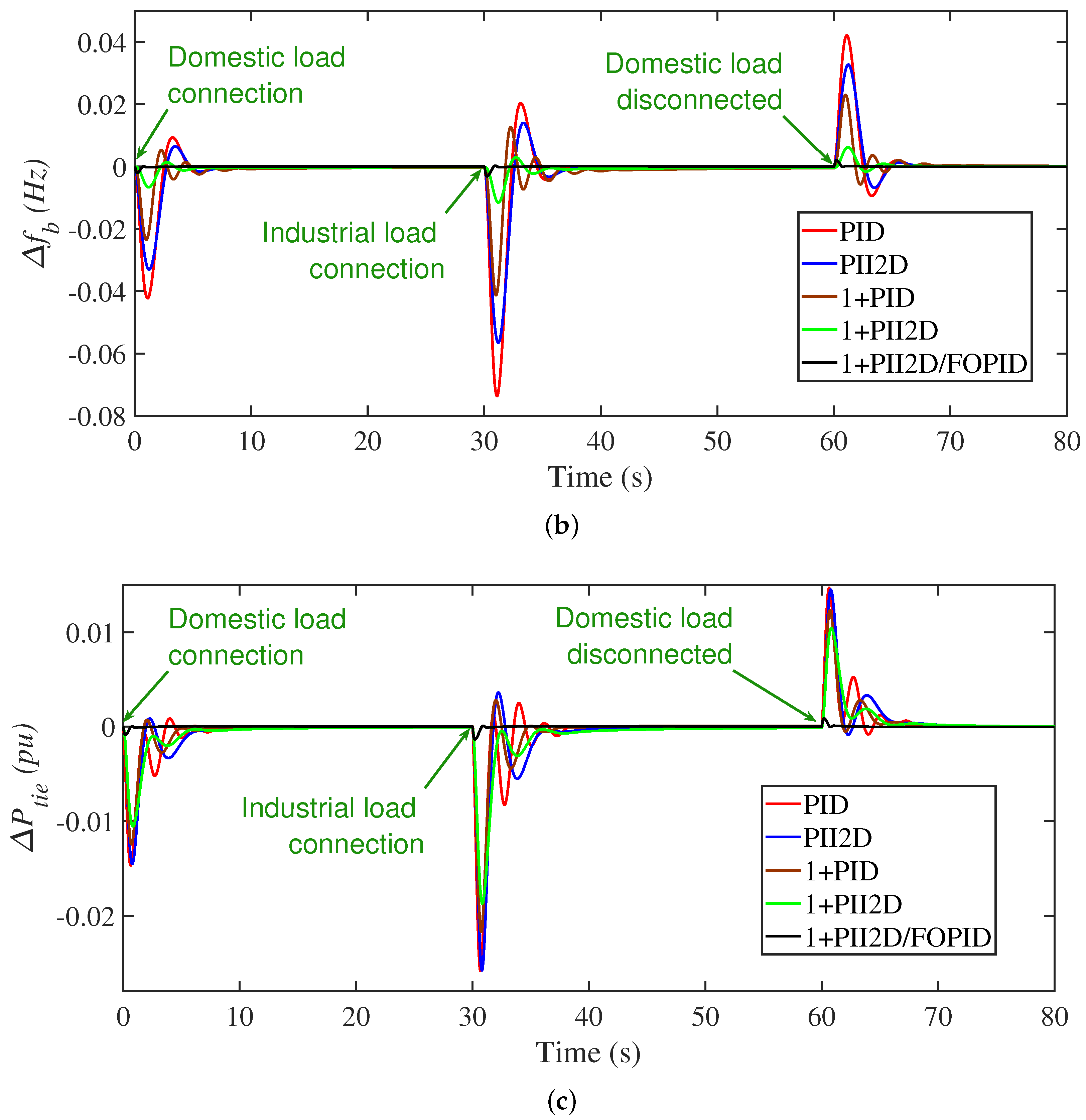
5.3. Scenario No. 3: The Impact of Domestic and Industrial Loads

The interconnected two-area systems may face some emergency cases, such as sudden connection and disconnection of domestic and industrial loads due to failure or disaster as seen in Figure 13. Therefore, the potential of the suggested coordination-based LFC and SMES using the 1+PII2D/FOPID controller based on the ARO algorithm is examined and revealed under the action of an extreme disturbance of different load types. For this purpose, the dynamic response of the system is studied when a domestic load is connected in area a at t = 0 s and then is disconnected at t = 60 s beside connecting the industrial load at t = 30 s. Figure 14 shows the variations in the system frequency and power for this scenario. It can be seen that the PID controller is dealing with this case as it has the highest frequency and power deviations and suffers from protracted damped vacillations. However, the PII2D controller gives damping characteristics better than the PID controller but with a long time for settling down deviations as noted in Table 4. Meanwhile, using the 1+PID and 1+PII2D controllers can face this severe failure of domestic and industrial loads and keep the system frequency within the permissible limits with undershoots of 0.05 Hz and 0.037 Hz at the instant of connecting the industrial load in area a, respectively. Moreover, the 1+PII2D is faster than 1+PID as it takes 16 s to retrieve the steady-state frequency, while the 1+PID controller lacks more than 22 s. From another side, the 1+PII2D/FOPID controllers have robust performance, with minimum MO, MU, and ST as summarized in Table 4. Hence, the proposed cascaded 1+PII2D/FOPID controller beside the SMES share in the LFC loop proved its dominance over the other control techniques in this drastic scenario of generation failure.

Figure 13. Loading profile at Scenario 3.

Figure 14. Obtained results at Scenario 3. (a) $\mathrm{\Delta }{f}_a$; (b) $\mathrm{\Delta }{f}_b$; (c) $\mathrm{\Delta }{P}_{tie}$.

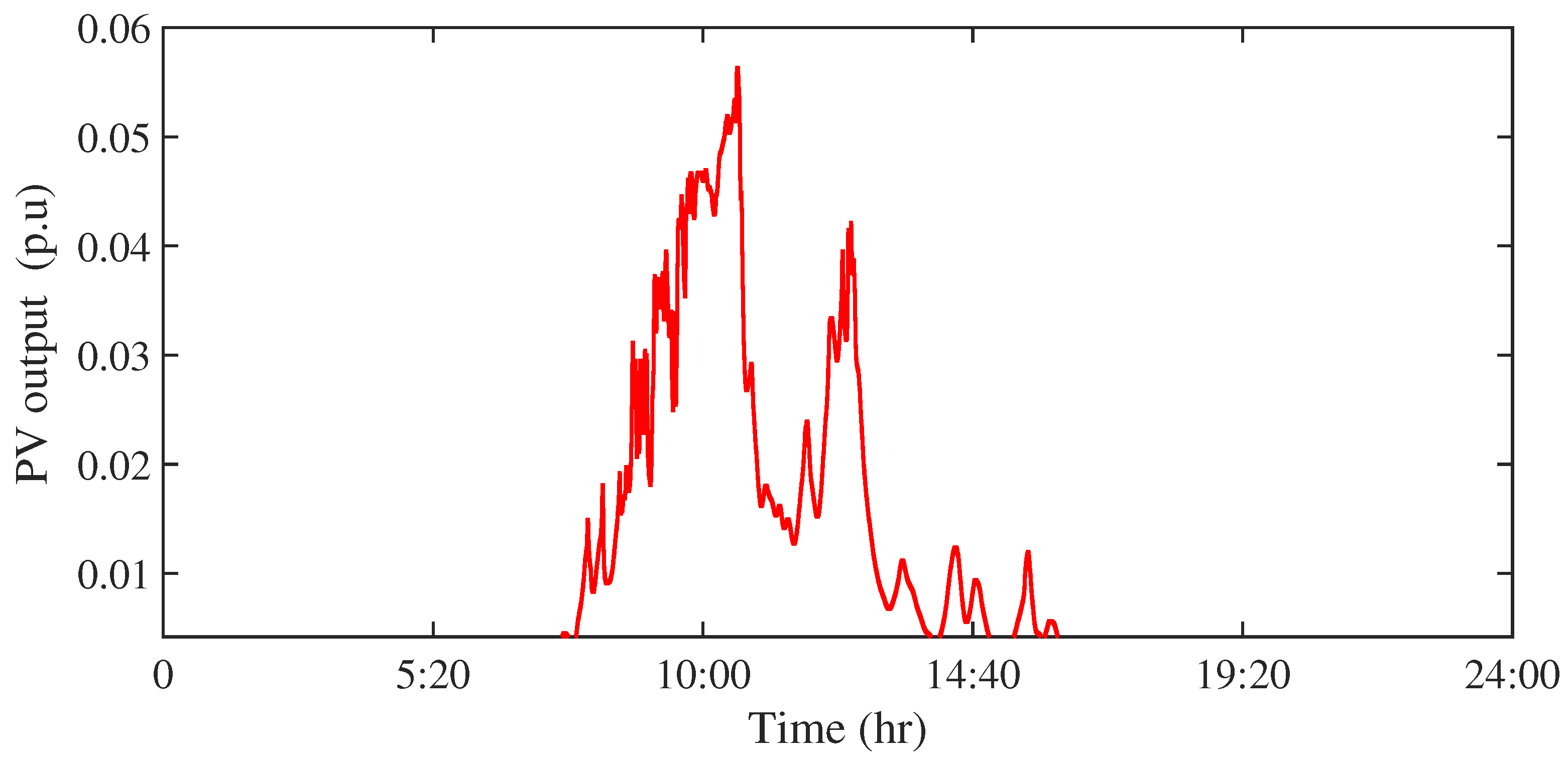
5.4. Scenario No. 4: The Impact of the PV Fluctuations

This context discusses the impact of the solar PV power plant on the frequency stability of the interconnected two-area power system. Hence, the effect of PV generation is considered in this case by applying a high fluctuated day of PV power from sunrise until the sunset as shown in Figure 15. Figure 16 clarifies the graphical illustrations of the system frequency and two-area exchange power deviations and the control effort achieved by applying the novel cascaded 1+PII2D/FOPID controller based on the ARO method. This figure shows that the proposed 1+PII2D/FOPID LFC guarantees lesser peaks and faster repression of the frequency and power oscillations detected due to the high oscillated power of PV generation plant than the other suggested classic and advanced controllers. Furthermore, the obtained results in Table 4 reveals the robustness of the 1+PII2D/FOPID control against other techniques in terms of the peak overshoot and undershoot and settling time during the whole period of supplying PV power to the loads. Therefore, this severe case proves that the proposed 1+PII2D/FOPID controller is the best at handling this issue compared to PID, I2D, 1+PID, and 1+PII2D controllers.

Figure 15. PV profile at Scenario 4.

Figure 16. Obtained results at Scenario 4. (a) $\mathrm{\Delta }{f}_a$; (b) $\mathrm{\Delta }{f}_b$; (c) $\mathrm{\Delta }{P}_{tie}$.

5.5. Scenario No. 5: The Impact of Wind Generation Fluctuations

The impact of the variability and intermittency of wind energy on the proposed two-area power system is studied to demonstrate the performance of the proposed cooperative of new 1+PII2D/FOPID controller based-LFC and SMES using the modified ARO technique. Hence, a wind farm in area a is connected to the system at t = 30 s and beside the 3% SLC at initial time as shown for the generation profile in Figure 17. The performance of all suggested controllers is depicted in Figure 18, whereas the system frequency deviates further by connecting the wind farm with the PID controller. Meanwhile, these deviations in frequency and power are damped slightly better with the PII2D controller than the PID controller. However, the two combined 1+PID and 1+PII2D controllers can suppress the high values of the system deviations with satisfactory performance compared to the previous controllers. Meanwhile, the 1+PII2D/FOPID controller can suppress the transient tie-line power oscillations to lower values compared to the other methods in addition to recording the minimum settling time when return to zero error. It is concluded from the results figure and Table 4 that the proposed ARO-1+PII2D/FOPID structure shows a robust performance against variations and uncertainty of wind generation and SLC in this scenario.

Figure 17. Wind profile at Scenario 5.

Figure 18. Obtained results at Scenario 5. (a) $\mathrm{\Delta }{f}_a$; (b) $\mathrm{\Delta }{f}_b$; (c) $\mathrm{\Delta }{P}_{tie}$.

6. Conclusions

A new hybrid fractional order-based LFC method is proposed in this paper based on the cascaded one plus proportional integral double-integral derivative (1+PII2D) cascaded with fractional order proportional-integral-derivative (FOPID), namely, the proposed 1+PII2D/FOPID controller. The proposed 1+PII2D/FOPID combines the cascaded structure and the 1+PII2D with FOPID non-integer control. The cascaded loops with added frequency signal are advantageous at better rejection of system disturbances. The inclusion of FOPID with its inherent added flexibility and freedom achieves better controller optimization. Moreover, a new application of ARO algorithm is presented in this paper for optimally determining the controller parameters. The proposed 1+PII2D/FOPID has been compared with featured controllers from the literature, including the PID, PII2D, 1+PID, and 1+PII2D controllers. Obtained results of two-area power grid with renewables, SMES devices, and hybrid HVDC/HVAC lines proved superior frequency response, and more stable, better disturbance rejection using the proposed 1+PII2D/FOPID controller.

References

1. Said, S.M.; Aly, M.; Balint, H. An Efficient Reactive Power Dispatch Method for Hybrid Photovoltaic and Superconducting Magnetic Energy Storage Inverters in Utility Grids. IEEE Access 2020, 8, 183708–183721. [Google Scholar] [CrossRef]
2. Maghami, M.R.; Mutambara, A.G.O. Challenges associated with Hybrid Energy Systems: An artificial intelligence solution. Energy Rep. 2023, 9, 924–940. [Google Scholar] [CrossRef]
3. Said, S.M.; Aly, M.; Hartmann, B.; Mohamed, E.A. Coordinated fuzzy logic-based virtual inertia controller and frequency relay scheme for reliable operation of low-inertia power system. IET Renew. Power Gener. 2021, 15, 1286–1300. [Google Scholar] [CrossRef]
4. Rameshar, V.; Sharma, G.; Bokoro, P.N.; Çelik, E. Frequency Support Studies of a Diesel–Wind Generation System Using Snake Optimizer-Oriented PID with UC and RFB. Energies 2023, 16, 3417. [Google Scholar] [CrossRef]
5. Kez, D.A.; Foley, A.M.; Ahmed, F.; Morrow, D.J. Overview of frequency control techniques in power systems with high inverter-based resources: Challenges and mitigation measures. IET Smart Grid 2023. [Google Scholar] [CrossRef]
6. Singh, B.; Slowik, A.; Bishnoi, S.K. Review on Soft Computing-Based Controllers for Frequency Regulation of Diverse Traditional, Hybrid, and Future Power Systems. Energies 2023, 16, 1917. [Google Scholar] [CrossRef]
7. Oshnoei, S.; Oshnoei, A.; Mosallanejad, A.; Haghjoo, F. Contribution of GCSC to regulate the frequency in multi-area power systems considering time delays: A new control outline based on fractional order controllers. Int. J. Electr. Power Energy Syst. 2020, 123, 106197. [Google Scholar] [CrossRef]
8. Elkasem, A.H.; Khamies, M.; Hassan, M.H.; Nasrat, L.; Kamel, S. Utilizing controlled plug-in electric vehicles to improve hybrid power grid frequency regulation considering high renewable energy penetration. Int. J. Electr. Power Energy Syst. 2023, 152, 109251. [Google Scholar] [CrossRef]
9. Aly, M.; Mohamed, E.A.; Noman, A.M.; Ahmed, E.M.; El-Sousy, F.F.M.; Watanabe, M. Optimized Non-Integer Load Frequency Control Scheme for Interconnected Microgrids in Remote Areas with High Renewable Energy and Electric Vehicle Penetrations. Mathematics 2023, 11, 2080. [Google Scholar] [CrossRef]
10. Said, S.M.; Mohamed, E.A.; Aly, M.; Ahmed, E.M. Enhancement of load frequency control in interconnected microgrids by SMES. In Superconducting Magnetic Energy Storage in Power Grids; Institution of Engineering and Technology: London, UK, 2022; pp. 111–148. [Google Scholar] [CrossRef]
11. Zhang, C.; Wang, S.; Zhao, Q. Distributed economic MPC for LFC of multi-area power system with wind power plants in power market environment. Int. J. Electr. Power Energy Syst. 2021, 126, 106548. [Google Scholar] [CrossRef]
12. Fathy, A.; Kassem, A.M. Antlion optimizer-ANFIS load frequency control for multi-interconnected plants comprising photovoltaic and wind turbine. ISA Trans. 2019, 87, 282–296. [Google Scholar] [CrossRef]
13. Patowary, M.; Panda, G.; Naidu, B.R.; Deka, B.C. ANN-based adaptive current controller for on-grid DG system to meet frequency deviation and transient load challenges with hardware implementation. IET Renew. Power Gener. 2017, 12, 61–71. [Google Scholar] [CrossRef]
14. Ali, M.; Kotb, H.; AboRas, M.K.; Abbasy, H.N. Frequency regulation of hybrid multi-area power system using wild horse optimizer based new combined Fuzzy Fractional-Order PI and TID controllers. Alex. Eng. J. 2022, 61, 12187–12210. [Google Scholar] [CrossRef]
15. Yakout, A.H.; Kotb, H.; Hasanien, H.M.; Aboras, K.M. Optimal Fuzzy PIDF Load Frequency Controller for Hybrid Microgrid System Using Marine Predator Algorithm. IEEE Access 2021, 9, 54220–54232. [Google Scholar] [CrossRef]
16. Rajesh, K.S.; Dash, S.S. Load frequency control of autonomous power system using adaptive fuzzy based PID controller optimized on improved sine cosine algorithm. J. Ambient. Intell. Humaniz. Comput. 2018, 10, 2361–2373. [Google Scholar] [CrossRef]
17. Mishra, D.; Sahu, P.C.; Prusty, R.C.; Panda, S. A fuzzy adaptive fractional order-PID controller for frequency control of an islanded microgrid under stochastic wind/solar uncertainties. Int. J. Ambient. Energy 2021, 43, 4602–4611. [Google Scholar] [CrossRef]
18. Fernández-Guillamón, A.; Gómez-Lázaro, E.; Muljadi, E.; Molina-García, Á. Power systems with high renewable energy sources: A review of inertia and frequency control strategies over time. Renew. Sustain. Energy Rev. 2019, 115, 109369. [Google Scholar] [CrossRef]
19. Pandey, S.K.; Mohanty, S.R.; Kishor, N. A literature survey on load–frequency control for conventional and distribution generation power systems. Renew. Sustain. Energy Rev. 2013, 25, 318–334. [Google Scholar] [CrossRef]
20. Yousri, D.; Babu, T.S.; Fathy, A. Recent methodology based Harris Hawks optimizer for designing load frequency control incorporated in multi-interconnected renewable energy plants. Sustain. Energy Grids Netw. 2020, 22, 100352. [Google Scholar] [CrossRef]
21. Dahab, Y.A.; Abubakr, H.; Mohamed, T.H. Adaptive Load Frequency Control of Power Systems Using Electro-Search Optimization Supported by the Balloon Effect. IEEE Access 2020, 8, 7408–7422. [Google Scholar] [CrossRef]
22. Shabani, H.; Vahidi, B.; Ebrahimpour, M. A robust PID controller based on imperialist competitive algorithm for load-frequency control of power systems. ISA Trans. 2013, 52, 88–95. [Google Scholar] [CrossRef]
23. El Yakine Kouba, N.; Menaa, M.; Hasni, M.; Boudour, M. Optimal load frequency control based on artificial bee colony optimization applied to single, two and multi-area interconnected power systems. In Proceedings of the 2015 3rd International Conference on Control, Engineering & Information Technology (CEIT), Tlemcen, Algeria, 25–27 May 2015; pp. 1–6. [Google Scholar] [CrossRef]
24. Ewais, A.M.; Elnoby, A.M.; Mohamed, T.H.; Mahmoud, M.M.; Qudaih, Y.; Hassan, A.M. Adaptive frequency control in smart microgrid using controlled loads supported by real-time implementation. PLoS ONE 2023, 18, e0283561. [Google Scholar] [CrossRef] [PubMed]
25. Youssef, A.R.; Mallah, M.; Ali, A.; Shaaban, M.F.; Mohamed, E.E.M. Enhancement of Microgrid Frequency Stability Based on the Combined Power-to-Hydrogen-to-Power Technology under High Penetration Renewable Units. Energies 2023, 16, 3377. [Google Scholar] [CrossRef]
26. Almasoudi, F.M.; Bakeer, A.; Magdy, G.; Alatawi, K.S.S.; Shabib, G.; Lakhouit, A.; Alomrani, S.E. Nonlinear coordination strategy between renewable energy sources and fuel cells for frequency regulation of hybrid power systems. Ain Shams Eng. J. 2023, 102399. [Google Scholar] [CrossRef]
27. Bakeer, M.; Magdy, G.; Bakeer, A.; Aly, M.M. Resilient virtual synchronous generator approach using DC-link capacitor energy for frequency support of interconnected renewable power systems. J. Energy Storage 2023, 65, 107230. [Google Scholar] [CrossRef]
28. Khalil, A.E.; Boghdady, T.A.; Alham, M.H.; Ibrahim, D.K. Enhancing the Conventional Controllers for Load Frequency Control of Isolated Microgrids Using Proposed Multi-Objective Formulation via Artificial Rabbits Optimization Algorithm. IEEE Access 2023, 11, 3472–3493. [Google Scholar] [CrossRef]
29. Neamah, N.M.; AbuHussein, A.; Hossam-Eldin, A.A.; Alghamdi, S.; AboRas, K.M. Improvement of Frequency Regulation of a Wind-Integrated Power System Based on a PD-PIDA Controlled STATCOM Tuned by the Artificial Rabbits Optimizer. IEEE Access 2023, 11, 55716–55735. [Google Scholar] [CrossRef]
30. AboRas, K.M.; Ragab, M.; Shouran, M.; Alghamdi, S.; Kotb, H. Voltage and frequency regulation in smart grids via a unique Fuzzy PIDD2 controller optimized by Gradient-Based Optimization algorithm. Energy Rep. 2023, 9, 1201–1235. [Google Scholar] [CrossRef]
31. Abid, S.; El-Rifaie, A.M.; Elshahed, M.; Ginidi, A.R.; Shaheen, A.M.; Moustafa, G.; Tolba, M.A. Development of Slime Mold Optimizer with Application for Tuning Cascaded PD-PI Controller to Enhance Frequency Stability in Power Systems. Mathematics 2023, 11, 1796. [Google Scholar] [CrossRef]
32. Sahu, R.; Panda, S.; Rout, U.K.; Sahoo, D. Teaching learning based optimization algorithm for automatic generation control of power system using 2-DOF PID controller. Int. J. Electr. Power Energy Syst. 2016, 77, 287–301. [Google Scholar] [CrossRef]
33. Dash, P.; Saikia, L.; Sinha, N. Automatic generation control of multi area thermal system using Bat algorithm optimized PD–PID cascade controller. Int. J. Electr. Power Energy Syst. 2015, 68, 364–372. [Google Scholar] [CrossRef]
34. Zhang, G.; Daraz, A.; Khan, I.A.; Basit, A.; Khan, M.I.; Ullah, M. Driver Training Based Optimized Fractional Order PI-PDF Controller for Frequency Stabilization of Diverse Hybrid Power System. Fractal Fract. 2023, 7, 315. [Google Scholar] [CrossRef]
35. Ayas, M.S.; Sahin, E. FOPID controller with fractional filter for an automatic voltage regulator. Comput. Electr. Eng. 2021, 90, 106895. [Google Scholar] [CrossRef]
36. Fathy, A.; Alharbi, A.G. Recent Approach Based Movable Damped Wave Algorithm for Designing Fractional-Order PID Load Frequency Control Installed in Multi-Interconnected Plants With Renewable Energy. IEEE Access 2021, 9, 71072–71089. [Google Scholar] [CrossRef]
37. Zaheeruddin; Singh, K. Load frequency regulation by de-loaded tidal turbine power plant units using fractional fuzzy based PID droop controller. Appl. Soft Comput. 2020, 92, 106338. [Google Scholar] [CrossRef]
38. Ahmed, E.M.; Mohamed, E.A.; Elmelegi, A.; Aly, M.; Elbaksawi, O. Optimum Modified Fractional Order Controller for Future Electric Vehicles and Renewable Energy-Based Interconnected Power Systems. IEEE Access 2021, 9, 29993–30010. [Google Scholar] [CrossRef]
39. Almasoudi, F.M.; Magdy, G.; Bakeer, A.; Alatawi, K.S.S.; Rihan, M. A New Load Frequency Control Technique for Hybrid Maritime Microgrids: Sophisticated Structure of Fractional-Order PIDA Controller. Fractal Fract. 2023, 7, 435. [Google Scholar] [CrossRef]
40. Zaid, S.A.; Bakeer, A.; Magdy, G.; Albalawi, H.; Kassem, A.M.; El-Shimy, M.E.; AbdelMeguid, H.; Manqarah, B. A New Intelligent Fractional-Order Load Frequency Control for Interconnected Modern Power Systems with Virtual Inertia Control. Fractal Fract. 2023, 7, 62. [Google Scholar] [CrossRef]
41. Aly, M.; Mohamed, E.A.; Ramadan, H.A.; Elmelegi, A.; Said, S.M.; Ahmed, E.M.; Shawky, A.; Rodriguez, J. Optimized LFC Design for Future Low-Inertia Power Electronics Based Modern Power Grids. In Proceedings of the 2023 IEEE Conference on Power Electronics and Renewable Energy (CPERE), Luxor, Egypt, 19–21 February 2023; pp. 1–6. [Google Scholar] [CrossRef]
42. Ahmed, E.M.; Selim, A.; Mohamed, E.A.; Aly, M.; Alnuman, H.; Ramadan, H.A. Modified manta ray foraging optimization algorithm based improved load frequency controller for interconnected microgrids. IET Renew. Power Gener. 2022, 16, 3587–3613. [Google Scholar] [CrossRef]
43. Mohamed, E.A.; Aly, M.; Elmelegi, A.; Ahmed, E.M.; Watanabe, M.; Said, S.M. Enhancement the Frequency Stability and Protection of Interconnected Microgrid Systems Using Advanced Hybrid Fractional Order Controller. IEEE Access 2022, 10, 111936–111961. [Google Scholar] [CrossRef]
44. Oshnoei, S.; Aghamohammadi, M.; Oshnoei, S.; Oshnoei, A.; Mohammadi-Ivatloo, B. Provision of Frequency Stability of an Islanded Microgrid Using a Novel Virtual Inertia Control and a Fractional Order Cascade Controller. Energies 2021, 14, 4152. [Google Scholar] [CrossRef]
45. Arya, Y.; Kumar, N.; Dahiya, P.; Sharma, G.; Çelik, E.; Dhundhara, S.; Sharma, M. Cascade-IλDμN controller design for AGC of thermal and hydro-thermal power systems integrated with renewable energy sources. IET Renew. Power Gener. 2021. [Google Scholar] [CrossRef]
46. Malik, S.; Suhag, S. A Novel SSA Tuned PI-TDF Control Scheme for Mitigation of Frequency Excursions in Hybrid Power System. Smart Sci. 2020, 8, 202–218. [Google Scholar] [CrossRef]
47. Babu, N.R.; Bhagat, S.K.; Chiranjeevi, T.; Pushkarna, M.; Saha, A.; Kotb, H.; AboRas, K.M.; Alsaif, F.; Alsulamy, S.; Ghadi, Y.Y.; et al. Frequency Control of a Realistic Dish Stirling Solar Thermal System and Accurate HVDC Models Using a Cascaded FOPI-IDDN-Based Crow Search Algorithm. Int. J. Energy Res. 2023, 2023, 9976375. [Google Scholar] [CrossRef]
48. El-Sousy, F.F.M.; Alqahtani, M.H.; Aljumah, A.S.; Aly, M.; Almutairi, S.Z.; Mohamed, E.A. Design Optimization of Improved Fractional-Order Cascaded Frequency Controllers for Electric Vehicles and Electrical Power Grids Utilizing Renewable Energy Sources. Fractal Fract. 2023, 7, 603. [Google Scholar] [CrossRef]
49. Ahmed, E.M.; Mohamed, E.A.; Selim, A.; Aly, M.; Alsadi, A.; Alhosaini, W.; Alnuman, H.; Ramadan, H.A. Improving load frequency control performance in interconnected power systems with a new optimal high degree of freedom cascaded FOTPID-TIDF controller. Ain Shams Eng. J. 2023, 14, 102207. [Google Scholar] [CrossRef]
50. Mohamed, E.A.; Ahmed, E.M.; Elmelegi, A.; Aly, M.; Elbaksawi, O.; Mohamed, A.A.A. An Optimized Hybrid Fractional Order Controller for Frequency Regulation in Multi-area Power Systems. IEEE Access 2020, 8, 213899–213915. [Google Scholar] [CrossRef]
51. Elmelegi, A.; Mohamed, E.A.; Aly, M.; Ahmed, E.M.; Mohamed, A.A.A.; Elbaksawi, O. Optimized Tilt Fractional Order Cooperative Controllers for Preserving Frequency Stability in Renewable Energy-Based Power Systems. IEEE Access 2021, 9, 8261–8277. [Google Scholar] [CrossRef]
52. Pathak, N.; Verma, A.; Bhatti, T.S.; Nasiruddin, I. Modeling of HVDC Tie Links and Their Utilization in AGC/LFC Operations of Multiarea Power Systems. IEEE Trans. Ind. Electron. 2019, 66, 2185–2197. [Google Scholar] [CrossRef]
53. Micev, M.; Ćalasan, M.; Oliva, D. Fractional Order PID Controller Design for an AVR System Using Chaotic Yellow Saddle Goatfish Algorithm. Mathematics 2020, 8, 1182. [Google Scholar] [CrossRef]
54. Motorga, R.; Mureșan, V.; Ungureșan, M.L.; Abrudean, M.; Vălean, H.; Clitan, I. Artificial Intelligence in Fractional-Order Systems Approximation with High Performances: Application in Modelling of an Isotopic Separation Process. Mathematics 2022, 10, 1459. [Google Scholar] [CrossRef]
55. Dulf, E.H. Simplified Fractional Order Controller Design Algorithm. Mathematics 2019, 7, 1166. [Google Scholar] [CrossRef]
56. Tejado, I.; Vinagre, B.; Traver, J.; Prieto-Arranz, J.; Nuevo-Gallardo, C. Back to Basics: Meaning of the Parameters of Fractional Order PID Controllers. Mathematics 2019, 7, 530. [Google Scholar] [CrossRef]
57. Mihaly, V.; Şuşcă, M.; Dulf, E.H. μ-Synthesis FO-PID for Twin Rotor Aerodynamic System. Mathematics 2021, 9, 2504. [Google Scholar] [CrossRef]
58. Wang, L.; Cao, Q.; Zhang, Z.; Mirjalili, S.; Zhao, W. Artificial rabbits optimization: A new bio-inspired meta-heuristic algorithm for solving engineering optimization problems. Eng. Appl. Artif. Intell. 2022, 114, 105082. [Google Scholar] [CrossRef]
59. Elshahed, M.; Tolba, M.A.; El-Rifaie, A.M.; Ginidi, A.; Shaheen, A.; Mohamed, S.A. An Artificial Rabbits’ Optimization to Allocate PVSTATCOM for Ancillary Service Provision in Distribution Systems. Mathematics 2023, 11, 339. [Google Scholar] [CrossRef]
60. Kumar, D.S.; Premkumar, M.; Kumar, C.; Muyeen, S. Optimal scheduling algorithm for residential building distributed energy source systems using Levy flight and chaos-assisted artificial rabbits optimizer. Energy Rep. 2023, 9, 5721–5740. [Google Scholar] [CrossRef]
61. Cao, Q.; Wang, L.; Zhao, W.; Yuan, Z.; Liu, A.; Gao, Y.; Ye, R. Vibration State Identification of Hydraulic Units Based on Improved Artificial Rabbits Optimization Algorithm. Biomimetics 2023, 8, 243. [Google Scholar] [CrossRef]