Auto- and Cross-Correlation Multifractal Analysis of Sea Surface Temperature Variability

Abstract

In this study, we investigate multiscale auto- and cross-correlation structural characteristics of sea surface temperature (SST) variability using our new methodology, called the multifractal asymmetric cross-correlation analysis (MF-ACCA), incorporating signs of a segment’s detrended covariance and linear trend. SST is greatly affected by air–sea interactions and the advection of water masses with a wide range of spatiotemporal scales. Since these force factors are imprinted on SST variability, their features can be revealed in terms of long-range auto- and cross-correlation structures of SST variability via a multifractal analysis. By applying the MF-ACCA methodology to SST variability in the East/Japan Sea, we have found the following features: (1) the auto- and cross-correlation multifractal features are dependent on several parameters, such as the location, linear trends (rising or falling), level of fluctuations, and temporal scales; (2) there are crossover behaviors that are discrete for small scales (less than 1000 days) but continuous for large scales (more than 1000 days); (3) long-range persistence of auto- and cross-correlations is random for large scales during the falling phase; (4) long-range persistence is stronger during the rising phase than during the falling phase; (5) the degree of asymmetry is greater for large scales than for small scales.

1. Introduction

In the climate system, the sea surface temperature (SST) is known as a proxy for various energy fluxes occurring on the sea’s surface via air–sea interactions [1]. Many climatic and physical processes are imprinted on the SST. That is, SST variability is indicative of a lateral energy transport by surface currents such as the geostrophic velocity and Ekman current velocity, a vertical energy transport by vertical entrainment and the Ekman pumping velocity, a turbulent energy flux via various air–sea interactions, and radiative flux. These factors have their own spatiotemporal dominant scales, and their impacts are region-specific. However, the dominant components contributing to SST variability have seasonality; that is, a peaked power is observed on an annual timescale. Also, there is a multi-decadal tendency to warmer SSTs, which is mainly due to greenhouse gas forces in the climate system [2].

Fractals and multifractals are ubiquitous in many diverse, complex systems, such as financial markets, brains, and climate systems. These concepts are very useful for describing the irregular or fragmented shape of natural features as well as other complex objects that are often characterized by spatial or time-domain statistical scaling laws and power-law behaviors of real-world physical systems, such as geophysics, biology, or fluid mechanics [3].

Most real-world systems are described by observable quantities in the form of a time series, and their fractal and multifractal properties are investigated by many time series analysis algorithms developed from multifractal formalism. The well-known Detrended Fluctuation Analysis (DFA) [4] and the Multifractal Detrended Fluctuation Analysis (MF-DFA) [5] have long been widely used to explore the long-range auto-correlation structures as well as multifractal features inherent in a singular nonstationary time series. Since the advent of DFA and MF-DFA, Podobnik and Stanley [6] have introduced the Detrended Cross-Correlation Analysis (DCCA) to detect the long-range persistence in the cross-correlations between synchronously observed nonstationary time series. Their methodology is used in a variety of scientific fields, including finance, physics, and earth sciences [7,8,9,10,11]. To explore the multifractal features in the cross-correlation structures of bivariate nonstationary time series, Zhou [12] proposed the Multifractal Detrended Cross-Correlation Analysis (MF-DCCA). MF-DCCA has been used in [13] to examine the cross-correlations between meteorological parameters and air pollution and in [14] to explore the cross-correlations between sunspot numbers and river flow fluctuations from a multifractal perspective.

The above methodologies have some shortcomings in revealing asymmetric features present in the scaling behavior of a time series, and MF-DCCA and the original DCCA algorithm naturally incorporate negative detrended covariances, leading to complex-valued fluctuation functions. In most applications, the latter difficulty was resolved by taking on the modulus of the covariance function in order to remove its negative sign. In most realistic cases, this operation can spuriously amplify the multifractal cross-correlation measure. In order to overcome these two limitations, the Multifractal Asymmetric Detrended Cross-Correlation Analysis (MF-ADCCA) [15] and the Multifractal Cross-Correlation Analysis (MFCCA) [16] were proposed for the former and the latter, respectively. In this study, we present the combined version of these two methods, called the Multifractal Asymmetric Cross-Correlation Analysis (MF-ACCA), which is used to investigate the auto- and cross-correlational structures of SST variability, more precisely, the SST anomaly (hereafter, SSTA) time series.

The East/Japan Sea (hereafter, EJS) is a semi-enclosed marginal sea surrounded by three adjacent countries, Korea, Russia, and Japan, as shown in Figure 1. According to previous studies [17,18,19,20], the SST variability in the EJS has a wide range of dominant timescales, from annual to multi-decadal scales, and the major contributors are known to be local wind anomalies, air–sea interactions, and the East Asian monsoon variability in generating interannual-to-decadal SST variability in the EJS [19,21]. Also, an El Niño-Southern Oscillation (ENSO) with a time scale of 3~7 years has been confirmed to be a significant factor in EJS SST long-term variability from various studies [22,23,24]. Overall, the dominant timescale in EJS SST variability has a wide range from 60–90 days and half a year [25] to the decadal scale [26] through inter-decadal timescales [18,19,27]. The major factors of EJS SST variability can be classified into two categories: air–sea interactions and the advection of water masses; seasonal variability is mainly due to the atmospheric forcing of the surface wind [28,29,30,31] and the transported volume of the Tsushima Warm Current (TWC) has a significant impact on SST variability in the southern part of the EJS [32,33].

In this study, we investigate the auto- and cross-correlation structures of SSTA in the EJS using two algorithms; one is the A-MFDFA as the multifractal version of asymmetric DFA (A-DFA) [34,35], and the other is the newly proposed multifractal asymmetric cross-correlation analysis (MF-ACCA); when considering two identical nonstationary time series, MF-ACCA becomes equivalent to A-MFDFA. First, in order to examine the non-universal properties of the auto-correlation multifractal features of SSTA, we apply the A-MFDFA algorithm to three selected study regions (Figure 1), namely E-line (East Korea Bay), S-line (western end of the Subpolar Front), and N-line (Nearshore Branch); also, the successive stations along each selected line can be utilized to examine the impact of geophysical distance. Second, in order to investigate the spatiotemporal scope of any dominant factors contributing to SST variability in terms of cross-correlation multifractal features, we apply the MF-ACCA algorithm to pairs of SSTA time series along all selected lines. It should be noted that the three study regions indicate different patterns of surface currents, as shown in Figure A1.

This article is organized as follows. In the section of Materials and Methods, a brief data description is presented, and we provide detailed explanations of multifractal analysis algorithms as well as a global wavelet spectral methodology. In the Analysis Results section, the analysis results are presented and described in detail. Lastly, in the Discussion and Conclusion sections, we evaluate our results in comparison with previous studies and present the direction of further research, especially on the extension of the study area and the causal relationship between other factors, such as heat fluxes on the surface and surface geostrophic currents estimated from sea surface height anomalies.

2. Materials and Methods

2.1. Data

The SST record used here was obtained from the National Oceanic and Atmospheric Administration (NOAA) Optimum Interpolation SST (OISST) version 2.1 software [36,37], with a horizontal resolution of 1/4° and a daily temporal resolution. By performing bias-correction on a satellite SST dataset using additional measurements, such as SSTs from the Argo float and buoy, and adopting revised correction methods, such as a ship–buoy SST correction algorithm and conversion method of the sea–ice concentration, the dataset quality has remarkably improved since 1 January 2016 [36,37]. Also, missing values in this long-term climate data of the NOAA 1/4° daily OISST were filled via interpolation for a spatially complete map of SST. The SSTA represents a departure from normal or average conditions and is computed by subtracting a 30-year duration climatological mean from each daily OISST value.

Since our goal in this study was to characterize the auto- and cross-correlation structures of SSTA, we used the limited database of a global gridded dataset confined to the EJS; the whole observation time was from 1 September 1981 to 4 April 2023. Since the total number of lattice points of the original gridded datasets was 1768, we considered the selected stations as shown in Figure 1 for the sake of computation time.

2.2. Multifractal Methodology

2.2.1. Multifractal Cross-Correlation Analysis (MFCCA)

This algorithm [16] allowed us to compute the arbitrary order covariance function of any two signals by properly incorporating the relative signs in the signals. The procedure of MFCCA is described as follows:

Step 1: Consider two time series $x_i$, $y_i$ for $i=\mathrm{1,2},\cdots ,N$ where $N$ is the length of the series. Then, we constructed the signal profile:

$$X\left(k\right)={\sum }_{i=1}^k\left[x_i-〈x〉\right],Y\left(k\right)={\sum }_{i=1}^k\left[y_i-〈y〉\right]$$

(1)

where $〈·〉$ denotes averaging over the entire time series.

Step 2: Both signal profiles were divided into $N_s=\mathrm{i}\mathrm{n}\mathrm{t}(N/s)$ disjoint segments $\mathsf{\nu }$ of length $s$. Because of the cases of the length N not being divided exactly by s, the segmentation procedure was repeated starting from the end of the signal. Thus, we obtained 2$N_s$ segments in total.

Step 3: For each segment $\nu$, the local trend was estimated by fitting a polynomial of order $m$ (${\tilde{X}}_{\nu }^{\left(m\right)}$ for $X$ and ${\tilde{Y}}_{\nu }^{\left(m\right)}$ for $Y$). In this study, we used a polynomial of order $m=2$. Then, the local trend was subtracted from the profile.

Step 4: The detrended cross-covariance within each segment was computed,

$$F_{XY}^2(\nu ,s)=\frac{1}{s}\sum _{k=1}^s\left\{\left(X\left[\left(\nu -1\right)s+k\right]-{\tilde{X}}_{\nu }^{\left(m\right)}\left(k\right)\right)\times \left(Y\left[\left(\nu -1\right)s+k\right]-{\tilde{Y}}_{\nu }^{\left(m\right)}\left(k\right)\right)\right\}$$

(2)

Compared to the detrended variance in the MF-DFA procedure [5], $F_{XY}^2(\nu ,s)$ takes both positive and negative values. Thus, we had to consider the sign of $F_{XY}^2(\nu ,s)$ when computing covariances of varying orders, $q$.

Step 5: The qth-order covariance function was computed by averaging across all segments,

$$F_{XY}^q\left(s\right)=\frac{1}{2N_s}{\sum }_{\nu =1}^{2N_s}\mathrm{s}\mathrm{g}\mathrm{n}\left(F_{XY}^2\left(\nu ,s\right)\right){\left|F_{XY}^2(\nu ,s)\right|}^{q/2},$$

(3)

where $\mathrm{s}\mathrm{g}\mathrm{n}\left(F_{XY}^2\left(\nu ,s\right)\right)$ denotes the sign of $F_{XY}^2(\nu ,s)$. Equation (3) held good only for any real number q except zero. In the case of $q=0$, the logarithmic version of Equation (3) was employed,

$$F_{XY}^0\left(s\right)=\frac{1}{4N_s}\sum _{\nu =1}^{2N_s}\mathrm{s}\mathrm{g}\mathrm{n}\left(F_{XY}^2\left(\nu ,s\right)\right)\ln \left|F_{XY}^2\left(\nu ,s\right)\right|$$

(4)

Step 6: The scaling behavior of the covariance function $F_{XY}^q\left(s\right)$, in the case that the function $F_{XY}^q\left(s\right)$ developed scaling, was manifested in the power-law dependence of $F_{XY}^q\left(s\right)$ as follows,

$${F_{XY}^q\left(s\right)}^{1/q}=F_{XY}(q,s)~s^{h_{XY}\left(q\right)}$$

(5)

where $h_{XY}\left(q\right)$, known as the generalized cross-correlation exponent, quantitatively characterized the fractal properties of the covariance. If $h_{XY}\left(q\right)$ was independent of q, the cross-correlation was said to be mono-fractal. In the case of multifractal cross-correlation, $h_{XY}\left(q\right)$ varied with q. Note that there was no fractal cross-correlation when $F_{XY}^q\left(s\right)$ fluctuated around zero. If both time series of $x_i$ and $y_i$ were identical, MFCCA became equivalent to MF-DFA.

2.2.2. Multifractal Asymmetric Detrended Cross-Correlation Analysis

The MF-ADCCA algorithm was first proposed to examine the asymmetric properties of the cross-correlations between two financial markets [15]; that is, when any one of two considered markets rose, there could be a different persistence for large and small fluctuations. The algorithm is a combination of MF-DCCA and A-DFA, and the procedure is described in detail below.

Step 1: Consider two time series $x_i$, $y_i$ for $i=\mathrm{1,2},\cdots ,N$ where $N$ is the length of the series. Then, their profiles were computed via a cumulative summation,

$$X\left(k\right)={\sum }_{i=1}^k\left[x_i-〈x〉\right],Y\left(k\right)={\sum }_{i=1}^k\left[y_i-〈y〉\right]$$

(6)

where $〈·〉$ denotes averaging over the entire time series, computed as $〈x〉=\frac{1}{N}\sum _{i=1}^N{x}_i$.

Step 2: We divided each of the time series {$x_i$, $y_i$} into $N_s=\mathrm{i}\mathrm{n}\mathrm{t}(N/s)$ non-overlapping segments of equal length $s$. Likewise, the profiles $\left\{X\left(k\right),Y\left(k\right)\right\}$ were also divided into $N_s=\mathrm{i}\mathrm{n}\mathrm{t}(N/s)$ non-overlapping segments of equal length $s$, respectively, and $\left\{x\left(t\right)\right\}$ into $N\left(s\right)=$ int$(N/s)$ non-overlapping segments of equal length s, respectively. In order to incorporate a short end part of the signal in the case that the record length $N$ was not divided by $s$, the same procedure was repeated from the end of the signal. Thus 2$N_s$ segments were obtained. Then, in the $\mathsf{\nu }$-th segment ($\nu =1,\cdots ,2N_s$), we have two pairs of segmented time series $\left\{x_{\nu }\left(k\right),X_{\nu }\left(k\right)\right\}$ and $\left\{y_{\nu }\left(k\right),Y_{\nu }\left(k\right)\right\}$ for $k=1,\cdots ,s$.

Step 3: For each segment time series of a pair of segmented time series $\left\{x_{\nu }\left(k\right),X_{\nu }\left(k\right)\right\}$, we computed the local linear fits (equivalent to local linear trends) $L_{\nu ,x} \mathrm{and} L_{\nu ,X}$ using the least squares regression, each of which is expressed as $L_{\nu ,x}=a_{\nu ,x}+b_{\nu ,x}k$ and $L_{\nu ,X}=a_{\nu ,X}+b_{\nu ,X}k$, respectively. In another pair of time series $\left\{y_{\nu }\left(k\right),Y_{\nu }\left(k\right)\right\}$, it was the same. The linear fit $L_{\nu ,x}$ was used to determine whether the trend of the $\nu$-th segment {$x_{\nu }\left(k\right)$} was positive (rising) or negative (falling), while the linear fit $L_{\nu ,X}$ was used to locally detrend the $\nu$-th profile segment {$X_{\nu }\left(k\right)$}. Thus, the detrended cross-covariance is computed as

$$F_{XY}^2(\nu ,s)=\frac{1}{s}\sum _{k=1}^s\left\{\left|X_{\nu }\left(k\right)-L_{\nu ,X}\left(k\right)\right|\times \left|Y_{\nu }\left(k\right)-L_{\nu ,Y}\left(k\right)\right|\right\}$$

(7)

Step 4: The detrended covariances {$F_{XY}^2(\nu ,s)$} were classified into two classes according to the piecewise trend of the corresponding time series $\left\{x_{\nu }\left(k\right),y_{\nu }\left(k\right)\right\}$, and the classified segments were used to assess the asymmetric cross-correlation scaling properties. As mentioned in Step 3, the local trend was determined by the sign of the slope $b_{\nu ,x}$ or $b_{\nu ,y}$. By, for example, taking the trend of {$x_i$}, we computed the so-called directional q-order detrended covariances as follows,

$$F_{XY}^{+}\left(q,s\right)={\left(\frac{1}{M^{+}}\sum _{\nu =1}^{2N_s}\frac{\mathrm{s}\mathrm{g}\mathrm{n}\left(b_{\nu ,x}\right)+1}{2}{\left[F_{XY}^2(\nu ,s)\right]}^{q/2}\right)}^{1/q}$$

(8)

$$F_{XY}^{-}\left(q,s\right)={\left(\frac{1}{M^{-}}\sum _{\nu =1}^{2N_s}\frac{\left[-\mathrm{s}\mathrm{g}\mathrm{n}\left(b_{\nu ,x}\right)+1\right]}{2}{\left[F_{XY}^2(\nu ,s)\right]}^{q/2}\right)}^{1/q}$$

(9)

where $M^{+}$ and $M^{-}$ denote the number of segments with positive and negative trends, respectively. In case $b_{\nu ,x}\ne 0$ for all segments, $M^{+}+M^{-}=2N_s$.

When the piecewise linear trend of $\left\{x\left(t\right)\right\}$ was ignored, the traditional MF-DCCA [12] was restored:

$$F_{XY}\left(q,s\right)={\left(\frac{1}{{2N}_s}\sum _{v=1}^{{2N}_s}{\left[F_{XY}^2(\nu ,s)\right]}^{q/2}\right)}^{1/q}$$

(10)

Thereby, if there are power-law cross-correlations, the following scaling law was established:

$$F_{XY}(q,s)~s^{h_{XY}\left(q\right)},F_{XY}^{+}(q,s)~s^{h_{XY}^{+}\left(q\right)},F_{XY}^{-}(q,s)~s^{h_{XY}^{-}\left(q\right)}$$

(11)

where $h_{XY}\left(q\right)$, $h_{XY}^{+}\left(q\right)$, and $h_{XY}^{-}\left(q\right)$ denote overall, rising-up, and falling-down scaling exponents, respectively. The scaling behaviors in Equation (11) were determined in the log–log plots, and the exponents were estimated via a linear fit over the scaling range.

In the case of q = 2, the exponent $h_{XY}\left(2\right)$ was interpreted in the same manner as the Hurst exponent. If $h_{XY}\left(2\right)>0.5$, the cross-correlation of both time series was said to be persistent, implying that an increase in one time series was followed by an increase in the other. When $h_{XY}\left(2\right)<0.5$, the cross-correlation was said to be anti-persistent, meaning that an increase in one signal was likely to be followed by a decrease in the other. The case of $h_{XY}\left(2\right)=0.5$ indicated a short-range or no cross-correlation. This interpretation was also valid in the MFCCA algorithm.

For the symmetricity of the cross-correlation of a pair of time series, the relation of $h_{XY}^{+}\left(q\right)=h_{XY}^{-}\left(q\right)$ indicated that the cross-correlation was symmetric. If $h_{XY}^{+}\left(q\right)\ne h_{XY}^{-}\left(q\right)$, the cross-correlation was said to be asymmetric, meaning that there was a trend-dependent scaling behavior. Further, the degree of cross-correlation asymmetry was measured via the following formula,

$${∆h_{XY}\left(q\right)=h}_{XY}^{+}\left(q\right)-h_{XY}^{-}\left(q\right).$$

(12)

The greater the magnitude of $∆h_{XY}\left(q\right)$, the more pronounced the asymmetry of the cross-correlation. The sign of $∆h_{XY}\left(q\right)$ indicated the dependence on the trending behavior of the chosen time series, herein {$x_i$}.

Generally, in these multifractal time series analysis algorithms, the q-order played the role of the microscope in the scaling behavior of detrended fluctuations (herein, the detrended covariance). For positive values of q, since the average $F_{XY}(q,s)$ was dominated by the segments with large covariance $F_{XY}^2(\nu ,s)$, the corresponding $h_{XY}\left(q\right)$ described the scaling behavior of the segments with large covarying fluctuations. On the contrary, for negative q, $h_{XY}\left(q\right)$ described the scaling behavior of small covarying fluctuations. All other scaling exponents, including $h_{XY}\left(q\right)$ in the MFCCA algorithm were equally interpreted.

2.2.3. Multifractal Asymmetric Cross-Correlation Analysis (MF-ACCA)

Since the detrended covariance of Equation (7) did not consider the sign of $F_{XY}^2(\nu ,s)$, there could be a limitation on taking a genuine covariance of the two signals, as stated in [16]. Thus, we replaced Equation (7) with Equation (2) and modified the directional q-order detrended covariances of Equations (8) and (9) into the following equations,

$$F_{XY}^{+}\left(q,s\right)={\left(\frac{1}{M^{+}}\sum _{\nu =1}^{2N_s}\mathrm{s}\mathrm{g}\mathrm{n}\left(F_{XY}^2(\nu ,s)\right)\frac{\mathrm{s}\mathrm{g}\mathrm{n}\left(b_{\nu ,x}\right)+1}{2}{\left|F_{XY}^2(\nu ,s)\right|}^{q/2}\right)}^{1/q}$$

(13)

$$F_{XY}^{-}\left(q,s\right)={\left(\frac{1}{M^{-}}\sum _{\nu =1}^{2N_s}\mathrm{s}\mathrm{g}\mathrm{n}\left(F_{XY}^2(\nu ,s)\right)\frac{\left[-\mathrm{s}\mathrm{g}\mathrm{n}\left(b_{\nu ,x}\right)+1\right]}{2}{\left|F_{XY}^2(\nu ,s)\right|}^{q/2}\right)}^{1/q}$$

(14)

In the presence of power-law cross-correlations, the scaling laws were the same as in Equation (11). In the cross-correlation analysis of the SSTA time series, we used the MF-ACCA algorithm. In the case that the two signals, {$x_i$, $y_i$}, were identical; the MF-ACCA algorithm was equivalent to A-MFDFA, which is a multifractal version of A-DFA.

2.3. Global Wavelet Spectrum

For the spectral analysis of SSTA, we performed a wavelet analysis on each time series by using the Morlet wavelet, a complex continuous wavelet with a zero mean [38], defined as

$${\psi }_0\left(\tau \right)={\pi }^{-1/4}{e}^{i\omega \tau }{e}^{-{\tau }^2/2}$$

(15)

where ω and τ represent the dimensionless frequency and time, respectively. In the case of ω = 6, the Morlet wavelet provided an optimal balance between time and frequency by yielding that its Fourier period, ${\mathrm{T}}_{\mathcal{F}}$, was close to its scale ($T_{\mathcal{F}}=1.03s$) [39]. In order to extract power spectral features from a single nonstationary time series, $x_n(n=\mathrm{1,2},\cdots ,N)$, we performed a continuous wavelet-transform (CWT) on the pair of $x_n$ and the scaled and normalized wavelet [40] in the manner of convolution. The used wavelet is expressed as

$$W_n^X(s)=\sqrt{\mathsf{\Delta }/s}\sum _{n\prime =1}^N{x}_{n\prime }{\psi }_0\left[\right(n\prime -n)\mathsf{\Delta }/s]$$

(16)

The wavelet power spectrum (WPS), ${\left|W_n^X\left(s\right)\right|}^2$, represents the power of a given single time series at a localized time-frequency point, and its complex argument can be interpreted as the local phase. By using the global wavelet spectrum (GWS) [41], defined as

$${\overline{W}}^2(s)=\frac{1}{N}\sum _{n=1}^N{\left|W_n^X\left(s\right)\right|}^2$$

(17)

where $N$ denotes the time duration, we find a dominant mode in a given time series.

3. Analysis Results

3.1. Spectral Pattern of SSTA

The SST variability in the upper-ocean mixed layer is governed by a variety of atmospheric and oceanic processes, and there are several dominant modes with different temporal scales. The spectral patterns of SSTA in all lattice points under study (Figure 1) are presented in Figure 2 in terms of GWS. As seen in Figure 1, two lines (E-line and N-line) extend from the coast towards the offshore area, and an annual scale (300~400 days) becomes apparent as going further away from the coast (Figure 2A,C); in particular, near the EKB, a multi-year scale (~1000 days) is dominant. Along S-Line (Figure 2B), the annual scaled mode is dominant over S2 through to S5 locations. It is noticeable that a wide bandwidth over 60 through 1000 days is observed at the N2 and N3 locations (Figure 2C) belonging to the Yamato basin. Although an annual scaled mode seems to be dominant overall, it should be noted that a spectral pattern is dependent on the region; generally, the current velocity is high near the coast, and an Ekman pumping is strong near the coast, too. These dynamical characteristics should be considered when interpreting the multifractal analysis results.

3.2. Multifractal Characteristics of SSTA

3.2.1. Multifractal Detrended Fluctuation Analysis

In this study, we investigated the multifractal features of SST variability using the MF-DFA algorithm, where the range of the order q is set to be from $-10$ to $+10$. Under the multifractal scaling, the generalized Hurst exponent $h\left(q\right)$ depends on the order q; $h\left(q\right)$ for $q<0$ is usually larger than $h\left(q\right)$ for $q>0$ [5]. Among various measures for quantifying the multifractality strength [42], we used a measure based on the generalized Hurst exponents, which reads

$$∆h=h_{max}-h_{min}=h\left(q_{min}\right)-h\left(q_{max}\right)$$

(18)

Although this measure is easy to adopt, there are some cases in which $h\left(q\right)$ is not a monotonic function of q [43], which is said to be an anomalous phenomenon. Thus, we used the following measure $∆h$, defined as [44]

$$∆h=\underset{q}{\max }h\left(q\right)-\underset{q}{\min }h\left(q\right)$$

(19)

In fact, since the proper determination of multifractal properties is greatly dependent on a good choice of scaling range, we should be cautious when applying these approaches. However, for practical purposes, we set two scaling ranges, say small scales from 30 to 1000 days and large scales from 1000 to 5000 days. Thereby, any variation in logarithmic plots of the fluctuation function based on detrended variance or covariance vs. the segment size was evaluated in terms of crossover behaviors.

Figure 3 shows the logarithmic plot of segment size vs. fluctuation functions of the order q over the segment range from 10 to 1000 days; for the sake of clarity, we considered three orders of q, such as $q_{min}=-10$, $q_{max}=+10$, and $q=2$. The multifractal strength, computed via Equation (19), is given in

Table 1. The generalized Hurst exponents and their multifractality strength are given for small scales from 10 to 1000 days.

Location	$\mathit{h}(+10)$	$\mathit{h}(+2)$	$\mathit{h}(-10)$	${∆\mathit{h}}^{\mathit{*}}$	Crossover Behavior
E1	0.93	1.04	1.4	0.47	not clear
E2	0.96	1.07	1.3	0.34	not clear
E3	0.84	0.96	1.22	0.38	not clear
E4	0.83	0.98	1.33	0.5	not clear
E5	0.76	0.92	1.2	0.44	not clear
S1	0.86	0.98	1.19	0.33	not clear
S2	0.79	0.93	1.22	0.43	weak
S3	0.75	0.9	1.3	0.55	strong
S4	0.64	0.84	1.29	0.65	strong
S5	0.65	0.84	1.32	0.67	strong
N1	0.82	0.96	1.19	0.37	weak
N2	0.89	0.98	1.24	0.35	not clear
N3	0.82	0.94	1.09	0.27	weak
N4	0.81	0.95	1.22	0.41	moderate
N5	0.65	0.84	1.32	0.67	strong

* The strength of multifractality is computed using Equation (19), for the scaling range from 30 to 1000 days.

. In terms of $h\left(2\right)$, a crossover behavior was clearly observed in some locations of S-line and N-line, which were mostly far from the coast, with the crossover scale near an annual scale (300~400 days). This behavior seems to be closely related to the dominant modes confirmed in the spectral analysis (Figure 2). Also, the strength of multifractality becomes larger further from the coast, especially along S-line (Table 1). Generally, two major contributions are known for the multifractality of a single time series: distribution and linear/nonlinear auto-correlation. Since the SSTA time series are nearly Gaussian-distributed, there could be a stronger nonlinear correlation in the underlying dynamics of SST variability far from the coast. In the estimation of the double logarithmic slope, the scaling range was almost mandatorily set to be from 30 to 1000 days. Thus, a concave or convex behavior of $F\left(s\right) \mathrm{v}\mathrm{s}. s$ against the corresponding fitted dotted line in Figure 3 can be a criterion of the crossover (Figure 3).

The multifractal behaviors over the large scaling range of 1000 to 5000 days are presented in Figure A2. In comparison with Figure 3, most slopes were lowered (Table 1 and

Table A1. The generalized Hurst exponents and its multifractality strength are given for large scales from 1000 to 5000 days.

Location	$\mathit{h}(+10)$	$\mathit{h}(+2)$	$\mathit{h}(-10)$	${∆\mathit{h}}^{\mathit{*}}$	Crossover Behavior
E1	0.86	0.84	0.82	0.04	not clear
E2	0.78	0.9	1.13	0.35	not clear
E3	0.86	0.88	1.08	0.22	not clear
E4	0.72	0.86	1.22	0.5	not clear
E5	0.9	0.89	1	0.1	not clear
S1	1.12	0.92	0.96	0.16	not clear
S2	1.05	0.95	1.01	0.04	strong (convex)
S3	0.85	0.79	0.69	0.16	strong (convex)
S4	0.99	0.81	0.61	0.38	not clear
S5	1.11	0.87	0.68	0.43	strong (convex)
N1	0.44	0.5	0.66	0.22	not clear
N2	0.41	0.56	0.89	0.48	not clear
N3	0.63	0.68	0.86	0.23	not clear
N4	1.29	1.1	1.11	0.18	strong (convex)
N5	1.11	0.87	0.68	0.43	weak (convex)

* The strength of multifractality is computed using Equation (19), for the scaling range from 1000 to 5000 days.

), indicating that there was a clear crossover between the small and large scales. Also, in terms of the Hurst exponent of $q(+2)$, two locations in N1 and N2 showed no persistence. These empirical results mean that the auto-correlation structure of SST variability was clearly non-universal. Another interesting finding is that the convex crossover behaviors were more salient (Figure A2B,C). This convexity led to a clear anomalous phenomenon; a negative generalized Hurst exponent was smaller than the positive one. Overall, multiple crossovers were present in the fractal/multifractal behaviors of SST variability.

The multifractality strength based on Equation (19) is presented in Table A1. Most locations showed weak multifractality, and some were nearly mono-fractal (E1, E5, S1, S2, S3, and N2). Thus, the SST variability showed a gradually weakening tendency of multifractality as the segment scale increased. This scale-dependent behavior seems to be related to the independence of forcing factors with different spatiotemporal scales [45], in which there was a clear distinction in the network’s topology between small and large temporal scales.

3.2.2. Asymmetric Multifractal Detrended Fluctuation Analysis

In this section, we investigated the asymmetric multifractal behaviors of SSTA using the A-MFDFA algorithm. In SST variability, the trend-sensitive dynamics are important to understand the underlying forces leading to rising and/or falling trends of the SST. To address this topic, A-MFDFA could be a good candidate. Figure 4 and Figure 5 show the asymmetric auto-correlation multifractal behaviors for small scales of 10 through to 1000 days.

Compared to Figure 3 and Figure A2, there was still crossover behavior, although it was dependent on locations. However, it is very clear that the crossover behavior became clearer as being further from the coast; S-line shows a clearer crossover than E- and N-lines. Another noticeable thing is that the crossover behavior was more conspicuous in negative A-MFDFA results than in positive ones (Figure 4 and Figure 5). The quantitative evaluations, multifractality and asymmetricity, are given in

Table 2. The multifractality strength and degree of asymmetry are given for rising and falling trend, respectively, for small scales from 10 to 1000 days.

Location	${∆\mathit{h}}^{+\mathit{*}}$	${∆\mathit{h}}^{-\mathbf{*}}$	$[\mathit{q}=+10]$			$[\mathit{q}=+2]$			$[\mathit{q}=-10]$
			${\mathit{h}}_{\mathit{a}\mathit{s}\mathit{y}}^{+}$	${\mathit{h}}_{\mathit{a}\mathit{s}\mathit{y}}^{-}$	${∆\mathit{h}}_{\mathit{a}\mathit{s}\mathit{y}}^{\mathit{*}\mathit{*}}$	${\mathit{h}}_{\mathit{a}\mathit{s}\mathit{y}}^{+}$	${\mathit{h}}_{\mathit{a}\mathit{s}\mathit{y}}^{-}$	${∆\mathit{h}}_{\mathit{a}\mathit{s}\mathit{y}}^{\mathit{*}\mathit{*}}$	${\mathit{h}}_{\mathit{a}\mathit{s}\mathit{y}}^{+}$	${\mathit{h}}_{\mathit{a}\mathit{s}\mathit{y}}^{-}$	${∆\mathit{h}}_{\mathit{a}\mathit{s}\mathit{y}}^{\mathit{*}\mathit{*}}$
E1	0.55	0.42	0.86	0.96	$-$0.1	0.99	1.09	$-$0.1	1.41	1.38	$+$0.03
E2	0.37	0.36	0.95	0.93	$+$0.02	1.08	1.03	0.05	1.32	1.29	0.03
E3	0.44	0.4	0.85	0.8	$+$0.05	0.99	0.93	0.06	1.29	1.2	0.09
E4	0.54	0.39	0.79	0.88	−0.09	0.97	0.99	−0.02	1.33	1.27	0.05
E5	0.39	0.48	0.78	0.74	0.04	0.93	0.92	0.01	1.17	1.22	−0.05
S1	0.39	0.29	0.81	0.91	−0.1	0.96	1	−0.04	1.2	1.2	0
S2	0.43	0.45	0.79	0.79	0	0.92	0.94	−0.02	1.22	1.24	−0.02
S3	0.53	0.56	0.73	0.78	−0.05	0.89	0.9	−0.01	1.26	1.34	−0.08
S4	0.66	0.65	0.64	0.65	−0.01	0.85	0.84	0.01	1.3	1.3	0
S5	0.61	0.71	0.68	0.65	0.03	0.85	0.83	0	1.29	1.36	−0.07
N1	0.37	0.38	0.81	0.86	−0.05	0.93	0.98	−0.05	1.18	1.27	−0.06
N2	0.38	0.32	0.9	0.88	0.02	0.97	0.98	−0.01	1.28	1.2	0.08
N3	0.29	0.43	0.83	0.76	0.07	0.94	0.92	0.02	1.12	1.19	−0.07
N4	0.38	0.46	0.82	0.77	0.05	0.97	0.93	0.04	1.2	1.23	−0.03
N5	0.61	0.71	0.68	0.65	0.03	0.85	0.85	0	1.29	1.36	−0.07

* The strength of multifractality for positive (rising) and negative (falling) trends, respectively, for the scaling range from 30 to 1000 days. ** The degree of asymmetricity is computed via Equation (12).

and

Table A2. The multifractality strength and degree of asymmetry are given for rising and falling trend, respectively, for large scales from 1000 to 5000 days.

Location	${∆\mathit{h}}^{+\mathit{*}}$	${∆\mathit{h}}^{-\mathbf{*}}$	$[\mathit{q}=+10]$			$[\mathit{q}=+2]$			$[\mathit{q}=-10]$
			${\mathit{h}}_{\mathit{a}\mathit{s}\mathit{y}}^{+}$	${\mathit{h}}_{\mathit{a}\mathit{s}\mathit{y}}^{-}$	${∆\mathit{h}}_{\mathit{a}\mathit{s}\mathit{y}}^{\mathit{*}\mathit{*}}$	${\mathit{h}}_{\mathit{a}\mathit{s}\mathit{y}}^{+}$	${\mathit{h}}_{\mathit{a}\mathit{s}\mathit{y}}^{-}$	${∆\mathit{h}}_{\mathit{a}\mathit{s}\mathit{y}}^{\mathit{*}\mathit{*}}$	${\mathit{h}}_{\mathit{a}\mathit{s}\mathit{y}}^{+}$	${\mathit{h}}_{\mathit{a}\mathit{s}\mathit{y}}^{-}$	${∆\mathit{h}}_{\mathit{a}\mathit{s}\mathit{y}}^{\mathit{*}\mathit{*}}$
E1	0.09	0.43	0.94	0.28	0.66	0.89	0.48	0.41	0.85	0.71	0.14
E2	0.29	0.56	0.78	0.7	0.08	0.87	0.88	−0.01	1.07	1.26	−0.19
E3	0.22	0.27	0.85	0.85	0	0.85	0.94	−0.09	1.07	1.12	−0.05
E4	0.39	0.48	0.73	0.76	−0.03	0.85	0.87	−0.02	1.12	1.24	−0.12
E5	0.05	0.21	0.9	0.82	0.08	0.87	0.88	−0.01	0.95	1.03	−0.08
S1	0.25	0.64	1.11	0.53	0.58	0.94	0.71	0.23	0.86	1.17	−0.31
S2	0.24	0.49	1.08	0.69	0.49	0.99	0.8	0.19	0.84	1.18	−0.34
S3	0.18	0.3	0.88	0.52	0.36	0.83	0.62	0.21	0.7	0.82	−0.12
S4	0.37	0.18	1	0.46	0.54	0.85	0.53	0.32	0.63	0.64	−0.01
S5	0.5	0.3	1.16	0.38	0.78	0.96	0.46	0.5	0.66	0.68	−0.02
N1	0.21	0.3	0.46	0.32	0.14	0.53	0.41	0.12	0.67	0.62	0.05
N2	0.51	0.43	0.38	0.46	−0.08	0.55	0.58	−0.03	0.89	0.89	0
N3	0.25	0.4	0.62	0.38	0.24	0.68	0.51	0.17	0.87	0.78	0.09
N4	0.16	0.3	1.29	0.63	0.66	1.18	0.71	0.47	1.13	0.93	0.2
N5	0.5	0.3	1.16	0.38	0.78	0.96	0.46	0.5	0.66	0.68	−0.02

* The strength of multifractality for positive (rising) and negative (falling) trends, respectively, for the scaling range from 1000 to 5000 days. ** The degree of asymmetricity is computed via Equation (12).

.

According to Table 2, the asymmetry looks weak or is nearly zero, meaning that there is no dependency of multifractality on trends. However, it should be noted that there was a clear crossover behavior. The scaling slope was estimated via a mandatory linear fitting over the determined scaling range, herein from 30 to 1000 days. Under the consideration of crossover behaviors, the asymmetric feature was said to be securely observed.

Figure A3 and Figure A4 show the asymmetric auto-correlation multifractal behaviors for large scales of 1000 through to 5000 days; in this case, the scaling range was set to be the whole range. Like the MF-DFA behaviors in Figure A2, the anomalous phenomenon was obviously seen along S-Line and two locations (N4 and N5) for the positive (rising) trend (Figure A3); this is also probably due to the strong convexity of fluctuation functions. In contrast, there was no anomalous behavior in the negative trend (Figure A4). This distinctive finding seems to imply that any forcing factors relating to a rising trend induce anomalous behavior.

Compared to the scaling behaviors in Figure 4, the tendency of no-persistence and weakly anti-persistence was certainly induced by the negative (falling) A-MFDFA components. This finding implies that there were clearly trend-dependent dynamics yielding distinct auto-correlation structures, especially in large temporal scales. These trend-dependent (asymmetric) dynamics seem to be closely related to the spatiotemporal scales of any dominant force, as reported in [45]. The quantitative descriptions of the degree of asymmetricity and strength of multifractality are given in Table A2 below.

Clearly, the asymmetric behavior was stronger for large scales compared to small scales. As for the strength of multifractality, there was an asymmetry for underlying trends. The degree of asymmetry was stronger in magnitude for the positive q-order than for the negative one. Also, there was directionality, meaning that the positive q-order was positively asymmetric, while the negative q-order seemed to be skewed into negative asymmetry. This order-dependent asymmetric behavior indicates that large fluctuations were governed more by the rising trend, while small fluctuations described by negative q-order were affected by the falling trend.

3.2.3. Multifractal Asymmetric Cross-Correlation Analysis (MF-ACCA)

In the previous section, we confirmed that the asymmetric multifractal behaviors were significantly distinguished for small and large scales; weak and no asymmetry was observed for small scales, while asymmetric behaviors were evidently observed for large scales. Further, the asymmetric feature was marked for large fluctuations described by positive q-orders, herein +2 and +10. These characteristics are related to the auto-correlation structure of SST variability.

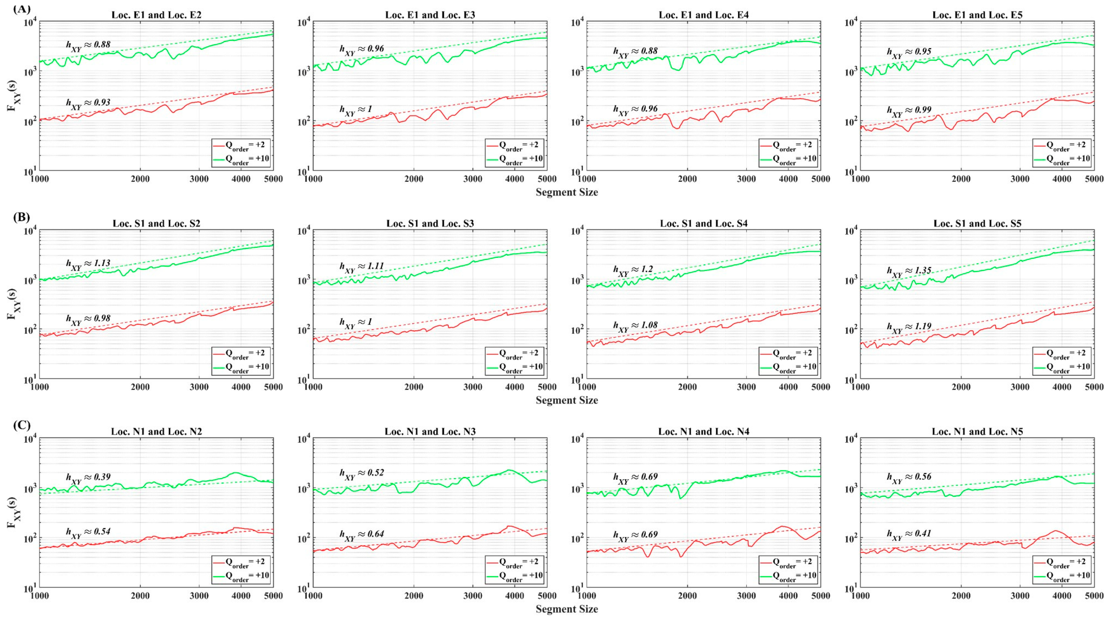
To examine the cross-correlation structures of SST variability, we conducted an MF-ACCA analysis on pairs of SSTA time series. For simplicity, we set the first locations of all considered study lines, say E-, S-, and N-lines, as the reference. That is, for positive (rising) and negative (falling) trends of reference points, the MF-ACCA was performed on the pairs consisting of a reference location and one of the other locations consecutively. Figure 6 and Figure A5 show the MF-ACCA results for small and large scales, respectively.

In the MF-ACCA analysis, there was no long-range persistent behavior for small fluctuations described by negative q-orders (Figure A6 and Figure A7). Thus, we considered only the two positive q-orders, +2 and +10. As confirmed in previous analysis results, the crossover behavior became clearer as being further from the coast. Also, overall, there was strong long-range persistent behavior, except for in N-line. As shown in Figure 1, N-line crossed the surface currents in the EJS (Figure A1), while two lines, E- and S-line, were closely related to the varying area of SPF. The SPF area showed seasonality in size and location [46], and the surface currents were nearly parallel in the two studied lines. Thus, the multifractal long-range cross-correlation behaviors can be interpreted as an indicator of advection factors in SST variability. Further, when comparing Figure 6C and Figure A5C, the temporal scales played a significant role in the cross-correlation structure; the persistence in long-range cross-correlation structures tended to become weaker, or there was no persistence as the temporal scale increased. This behavior is consistent with previous results of MF-DFA and A-MFDFA analyses.

Also, there was a concavity in the scaling behaviors for small scales (Figure 6), while a convex behavior was observed for large scales (Figure A5). This behavior was also consistent with previous results of MF-DFA and A-MFDFA analyses. The quantitative description of the strength of the multifractality of cross-correlation structures is provided in

Table 3. Table for multifractality strength, in terms of Equation (19), of pairs of locations corresponding to Figure 6 and Figure A5.

Location	Small Scales from 10 to 1000 Days			Large Scales from 1000 to 5000 Days
	${\mathit{h}}_{\mathit{X}\mathit{Y}}(+10)$	${\mathit{h}}_{\mathit{X}\mathit{Y}}(+2)$	${{∆\mathit{h}}_{\mathit{X}\mathit{Y}}}^{\mathit{*}}$	${\mathit{h}}_{\mathit{X}\mathit{Y}}(+10)$	${\mathit{h}}_{\mathit{X}\mathit{Y}}(+2)$	${{∆\mathit{h}}_{\mathit{X}\mathit{Y}}}^{\mathit{*}\mathit{*}}$
E12	0.93	1.07	0.14	0.88	0.93	0.05
E13	0.83	1	0.17	0.96	1	0.04 0.08
E14	0.81	0.99	0.17	0.88	0.96
E15	0.77	0.99	0.22	0.95	0.99	0.04
S12	0.82	1	0.18	1.13	0.98	0.15
S13	0.73	0.94	0.21	1.11	1	0.11
S14	0.66	0.87	0.21	1.2	1.08	0.12
S15	0.66	0.88	0.22	1.35	1.19	0.16
N12	0.87	0.99	0.12	0.39	0.54	0.15
N13	0.79	0.94	0.15	0.52	0.64	0.12
N14	0.76	0.95	0.19	0.69	0.69	0
N15	0.73	0.93	0.2	0.56	0.41	0.15

* The scaling range is from 30 to 1000 days. ** The scaling range is from 1000 to 5000 days.

.

In order to examine the influence of linear trends on scaling behaviors, we conducted the MF-ACCA analysis on all considered pairs of SSTA. Figure 7 and Figure 8 show the MF-ACCA results for small scales of 10 through to 1000 days. For small scales, there were no noticeable distinctions compared to previous results; all generalized Hurst exponents showed a stable, persistent behavior, and there was no anomalous phenomenon, irrespective of the linear trends. Overall, the scaling behavior was concave for all trends.

Still, a crossover behavior became marked as being far away from the coast, and the crossover seemed to be clearer in the negative (falling) trend than in the positive (rising) trend. The quantitative descriptions of the degree of asymmetry and the strength of the multifractal cross-correlation structure are given in

Table 4. The multifractality strength and degree of asymmetry of cross-correlation structure of SSTA are given for rising and falling trend, respectively, for small scales from 10 to 1000 days.

Pairs	${∆\mathit{h}}_{\mathit{X}\mathit{Y}}^{+\mathit{*}}$	${∆\mathit{h}}_{\mathit{X}\mathit{Y}}^{-\mathit{*}}$	$[\mathit{q}=+10]$			$[\mathit{q}=+2]$
			${\mathit{h}}_{\mathit{X}\mathit{Y}}^{+}$	${\mathit{h}}_{\mathit{X}\mathit{Y}}^{-}$	${∆\mathit{h}}_{\mathit{X}\mathit{Y}}^{\mathit{*}\mathit{*}}$	${\mathit{h}}_{\mathit{X}\mathit{Y}}^{+}$	${\mathit{h}}_{\mathit{X}\mathit{Y}}^{-}$	${∆\mathit{h}}_{\mathit{X}\mathit{Y}}^{\mathit{*}\mathit{*}}$
E12	0.13	0.17	0.92	0.92	0	1.05	1.09	−0.04
E13	0.15	0.2	0.85	0.79	0.06	1	0.99	0.01
E14	0.18	0.17	0.79	0.85	−0.06	0.97	1.02	−0.05
E15	0.21	0.22	0.77	0.78	−0.01	0.98	1	−0.02
S12	0.17	0.19	0.79	0.84	−0.05	0.96	1.03	−0.07
S13	0.21	0.19	0.68	0.81	−0.13	0.89	1	−0.11
S14	0.21	0.19	0.61	0.74	−0.13	0.82	0.93	−0.11
S15	0.22	0.2	0.61	0.74	−0.13	0.83	0.94	−0.11
N12	0.1	0.13	0.86	0.88	−0.02	0.96	1.01	−0.05
N13	0.12	0.19	0.8	0.76	0.04	0.92	0.95	−0.03
N14	0.17	0.19	0.76	0.78	−0.02	0.93	0.97	−0.04
N15	0.18	0.2	0.74	0.72	0.02	0.92	0.92	0

* The strength of multifractality for positive (rising) and negative (falling) trends, respectively, for the scaling range from 30 to 1000 days. ** The degree of asymmetricity is computed via Equation (12).

below.

As clearly shown in Table 4, the multifractality of the cross-correlation structure was weak, and the asymmetry was slightly skewed into a negative (falling) trend. Since we considered only the large fluctuations by a positive q-order, the weak negatively asymmetric behavior indicates that small-scaled forcing factors were nearly symmetric, although they had greater effects during linearly falling phases.

Figure A8 and Figure A9 show the MF-ACCA results for large scales of 1000 through to 5000 days; the scaling range was set to be the whole range. An anomalous phenomenon was observed in the positive (rising) trend only along S-line. A strong convex scaling behavior was observed in the negative (falling) trend along E-line; an interesting inflective variation with a convex-to-concave pattern was observed along S-line. In fact, these behaviors are closely related to the complex surface current patterns because the study area belongs to the varying SPF regions. Also, along N-line, no- and anti-persistent behaviors are consistent with previous results of an A-MFDFA analysis.

When closely examining Figure A9A, an anomalous behavior could be masked due to a strong convexity in the scaling behavior. Thus, the determination of anomalous behavior should be deferred. The quantitative descriptions are presented in

Table A3. The multifractality strength and degree of asymmetry of cross-correlation structure of SSTA are given for rising and falling trend, respectively, for large scales from 1000 to 5000 days.

Pairs	${∆\mathit{h}}_{\mathit{X}\mathit{Y}}^{+\mathit{*}}$	${∆\mathit{h}}_{\mathit{X}\mathit{Y}}^{-\mathit{*}}$	$[\mathit{q}=+10]$			$[\mathit{q}=+2]$
			${\mathit{h}}_{\mathit{X}\mathit{Y}}^{+}$	${\mathit{h}}_{\mathit{X}\mathit{Y}}^{-}$	${∆\mathit{h}}_{\mathit{X}\mathit{Y}}^{\mathit{*}\mathit{*}}$	${\mathit{h}}_{\mathit{X}\mathit{Y}}^{+}$	${\mathit{h}}_{\mathit{X}\mathit{Y}}^{-}$	${∆\mathit{h}}_{\mathit{X}\mathit{Y}}^{\mathit{*}\mathit{*}}$
E12	0.05	0.13	0.87	0.59	0.28	0.92	0.72	0.2
E13	0.02	0.16	0.94	0.64	0.3	0.96	0.8	0.16
E14	0.03	0.27	0.88	0.61	0.27	0.91	0.88	0.03
E15	0.02	0.3	0.92	0.69	0.23	0.9	0.99	−0.09
S12	0.14	0.14	1.13	0.67	0.46	0.99	0.84	0.15
S13	0.11	0.26	1.14	0.55	0.59	1.03	0.81	0.22
S14	0.13	0.33	1.24	0.39	0.84	1.1	0.72	0.38
S15	0.2	0.38	1.4	0.07	1.33	1.2	0.45	0.75
N12	0.16	0.17	0.41	0.28	0.13	0.57	0.45	0.12
N13	0.11	0.19	0.5	0.35	0.15	0.61	0.54	0.07
N14	0.03	0.15	0.71	0.28	0.43	0.68	0.43	0.25
N15	0.11	0.22	0.6	0.11	0.49	0.49	−0.11	0.6

* The strength of multifractality for positive (rising) and negative (falling) trends, respectively, for the scaling range from 1000 to 5000 days. ** The degree of asymmetricity is computed via Equation (12).

below. For large scales, a strong asymmetric behavior was observed for almost all pairs, which was especially stronger in large fluctuations (q = +10). This behavior seems to strongly state that a positive (rising) trend derived from large-scale forcing was dominant in the SST variability of EJS. Compared to previous studies on global warming, our results show that the warming force could be significantly influenced by large-scale forcing factors.

4. Discussion

In this study, we examined the auto- and cross-correlation structures of SST variability in the EJS in terms of multifractal time series analysis methodologies. In order to avoid the spuriousness in evaluating the cross-correlation structure and evaluate the impact of linear trends on the long-range correlation structures, we presented a new MF-ACCA algorithm, combining two algorithms, MFCCA [16] and MF-ADCCA [15]. The MF-ACCA algorithm retrieves the A-MFDFA when applied to two identical time series. Thus, by applying the MF-ACCA to a singular SSTA time series and its pairs, we obtained some noteworthy findings on auto- and cross-correlation structures of SST variability in the EJS.

Three studied regions in the EJS were selected in order to distinctly investigate the effect of atmospheric and oceanic processes on multifractal features of SST variability; as seen in Figure A1, E-line extended from the coast toward the offshore area, S-line captured well the time-varying SPF currents, and N-line crossed the three branches of the Tsushima warm current (TWC). The SST variability in the EKB, indicated by E-line (E1 through E3), is dominantly described by interannual forcing factors (Figure 2A) and is known to be associated with the eddy-like circulation anomaly via the Arctic Oscillation (AO)-related wind forcing [47]. The SPF region, indicated by S-line, had a strong seasonality in spatial scope [48], and its eastern end part spatiotemporally varied [46]. As observed in Figure 2B, the annual forcing became stronger as it moved away from the eastern end of the SPF. Since N-line is located in the southern part of EJS near the Korea–Tsushima Strait (KTS) and crosses the western branches of TWC, it could be greatly affected by the TWC transport [32]. Thus, the auto- and cross-correlation structures of the SSTA time series on those regions provide us with information on dominant underlying forcing factors, leading to long-range persistence depending on spatiotemporal scales.

The presence of multifractality in SST variability meant that there were auto- and cross-correlation structures depending on the fluctuation levels; the large positive q-value denotes large fluctuations, while the large negative q-value denotes small fluctuations. As shown in Table 1 and Table A1, although being a long-range persistence in most locations, there was a difference in the degree of persistence, indicated by the generalized Hurst exponent, and strength of multifractality when comparing the analysis results for small and large scales; this difference strongly indicates that there was a scale-specific forcing factor underlying the SST variability. A discrete or continuous crossover behavior also supports the presence of scale-specific forcing.

The linear trend of SST variability was location- and scale-dependent. Thus, there can be asymmetric features in the auto- and cross-correlation structures. Table 2 and Table A2 show that the asymmetry in the auto-correlation structure was scale-dependent; there was nearly symmetry in the positive (rising) and negative (falling) trends for small scales, while a considerable asymmetry was seen for large scales. Also, the asymmetry in the auto-correlations was dependent on the fluctuation levels (Table A2); large fluctuations had a stronger persistence during positive (rising) trends, while small fluctuations had a stronger persistence during negative (falling) trends. These results imply that there were scale- and trend-dependent dynamics underlying the SST variability.

The multifractal features in the cross-correlation structures were strongly long-range persistent for the whole scales from 30 to 5000 days, except for pairs of SSTA time series along N-line (Table 3), where weak or nearly no persistence appeared for large scales. Also, the relatively small multifractality was mainly due to the absence of long-range cross-correlations for negative q-values (Figure A6 and Figure A7); DCCA [6] and MFCCA [16] algorithms regard the covariance functions fluctuating around zero as no cross-correlation.

The asymmetry in cross-correlation multifractal features (Table 4 and Table A3) was very similar to that in the auto-correlation multifractal features (Table 2 and Table A2). The degree of asymmetry was greater in the large scales than in the small scales, and the directionality was the same; for large scales, the asymmetry skewed toward a positive (rising) trend while being skewed toward a negative (falling) trend for small scales. This scale-dependent asymmetry directionality could be closely related to climate change, especially a global warming trend. Although there is no direct evidence supporting the causality, it can be argued that any force leading to a positive (rising) trend in SST variability has a large scale (more than 1000 days) and shows a more persistent behavior during a rising phase than during a falling phase.

In a recent study [49], a warm bias in cold SST ($-2\mathrm{℃}\mathrm{t}\mathrm{o}10\mathrm{℃})$ was reported in the EJS. However, since we deal with an SST anomaly dataset detrended by climatology, the warm bias problem is not a critical matter in our analysis results. Also, the warm bias was mainly restricted to the northern and north-western parts of EJS; only a part of S-line was incorporated.

5. Conclusions

The analysis results in this study can be categorized into two parts: an auto-correlation structure and a cross-correlation structure of SST variability. As for the auto-correlation, the results of the MF-DFA and A-MFDFA analyses are found in Figure 3, Figure 4 and Figure 5 (Figure A2, Figure A3 and Figure A4), along with Table 1 and Table 2 (Table A1 and Table A2). Their summary is as follows:

• Overall, the long-range auto-correlation was strongly persistent for the whole scale from 30 to 5000 days, meaning that the Hurst exponent $h(+2)$ was very close to 1. However, two locations of N1 and N2 near the KTS seemed to be random only for large scales from 1000 to 5000 days; their Hurst exponents were nearly 0.5 (Table A1).
• All considered SSTAs from different locations show scale- and location-dependent multifractal features (Table 1 and Table 2); the strength of multifractality was greater for small scales (30–1000 days) than for large scales (1000–5000 days), with the strongest in the S-line region (near the SPF) for small scales.
• A distinct crossover behavior appeared along S-line (SPF region), with an annual crossover scale (300–400 days), through which a long-range persistence changed into anti- or no-persistence for small scales (Figure 3). For large scales, the crossover behavior seemed continuous; a convex functional form was observed (Figure A2).
• All the asymmetric long-range auto-correlations were strongly persistent for small scales (Table 2), while some locations showed random behaviors (Table A2). The random behavior of auto-correlation structures for large scales was observed more frequently in negative (falling) trends than in positive (rising) trends.
• The crossover behaviors in the A-MFDFA analysis were the same as those in the MF-DFA analysis.
• The degree of asymmetry for three q-order detrended fluctuation functions was greater for large scales (1000 to 5000 days) than for small scales (30 to 1000 days); there seems to be nearly no asymmetry for small scales. As for the asymmetry of large scales, large fluctuations (with positive q-values, $+2$ and $+10$) showed a strong positive asymmetry, while small fluctuations (with negative q-value, $-10$) showed a weak or moderate negative asymmetry.

The analysis results concerning the cross-correlation structures are given in Figure 6, Figure 7 and Figure 8 (Figure A9) as well as Table 2 and Table 3 (Table A3). They are summarized as follows:

• There was no long-range cross-correlation for small fluctuations, indicated by negative q-values (Figure A6 and Figure A7).
• Most pairs showed a strong long-range cross-correlation structure for small and large scales, which was indicated by the Hurst exponent $h_{XY}(+2)$ of nearly one (Table 3); cross-correlation pairs along N-line showed considerably weak-persistent or random behavior only for large scales (Table 3).
• Among weak crossover behaviors observed for small scales (Figure 6), N-line showed a relatively stronger crossover behavior (Figure 6C) with an annual crossover scale, indicating that there was a distinct difference in underlying forces between two remote locations (N1 and N4 and N1 and N5).
• The strength of multifractality was a little stronger in the small scales than in the large scales; note that the overall weak multifractality was mainly due to the absence of long-range cross-correlations for negative q-values.
• Most asymmetric long-range cross-correlations were strongly persistent for small and large scales, characterized by the Hurst exponent of nearly one for both positive (rising) and negative (falling) trends. However, N-line clearly deviated from these persistent behaviors, especially for large scales (Table A3); the Hurst exponents were close to 0.5, indicating the randomness in cross-correlations, and the negative (falling) Hurst exponents were less persistent than the positive (rising) ones.
• The degree of asymmetry for two positive q-order detrended fluctuation functions was greater for large scales (1000 to 5000 days) than for small scales (30 to 1000 days). As for the directionality of asymmetry, there was a weak negative skewed asymmetry in the small scales, while a strong positive skewed asymmetry was observed in large scales (Table 4 and Table A3).

We found some noticeable multifractal features in auto- and cross-correlations of SST variability using a combined algorithm, MF-ACCA. There was clearly scale- and location-dependent long-range persistence in auto- and cross-correlation structures; however, no concrete underlying forcing factors were revealed. It would be valuable to quantify the degree of causal relations between SST variability and representative forcing factors, such as advective forces relating to the surface currents and the air–sea interactions; the advective forces can be indicated as the geostrophic currents by the sea surface heights (SSH), and the air–sea interactions could be related to wind stresses and heat fluxes. These topics will be studied in future research using a multifractal time series analysis methodology. Also, examining scale-dependent structures of long-range cross-correlations in the EJS can enhance our understanding of the evolutionary features of climate change in marginal seas.

References

- Deser, C.; Alexander, M.A.; Xie, S.-P.; Phillips, A.S. Sea Surface Temperature Variability: Patterns and Mechanism. Annu. Rev. Mar. Sci. 2010, 2, 115–143. [Google Scholar] [CrossRef] [PubMed]
- Bulgin, C.E.; Merchant, C.J.; Ferreira, D. Tendencies, variability and persistence of sea surface temperature anomalies. Sci. Rep. 2020, 10, 7986. [Google Scholar] [CrossRef] [PubMed]
- Lopes, R.; Betrouni, N. Fractal and multifractal analysis: A review. Med. Image Anal. 2009, 13, 634–649. [Google Scholar] [CrossRef] [PubMed]
- Peng, C.-K.; Buldyrev, S.V.; Havlin, S.; Simons, M.; Stanley, H.E.; Goldberger, A.L. Mosaic organization of DNA nucleotides. Phys. Rev. E 1994, 49, 1685. [Google Scholar] [CrossRef] [PubMed]
- Kantelhardt, J.W.; Zschiegner, S.A.; Bunde, E.K.; Havlin, S.; Bunde, A.; Stanley, H.E. Multifractal detrended fluctuation anal-ysis of nonstationary time series. Phys. A 2002, 316, 87–114. [Google Scholar] [CrossRef]
- Podobnik, B.; Stanley, H.E. Detrended Cross-Correlation Analysis: A New Method for Analyzing Two Nonstationary Time Series. Phys. Rev. Lett. 2008, 100, 084102. [Google Scholar] [CrossRef] [PubMed]
- Gvozdanovic, I.; Podobnik, B.; Wang, D.; Eugene Stanley, H. 1/f behavior in cross-correlations between absolute returns in a US market. Phys. A 2012, 391, 2860–2866. [Google Scholar] [CrossRef]
- Horvatic, D.; Stanley, H.E.; Podobnik, B. Detrended cross-correlation analysis for non-stationary time series with periodic trends. Europhys. Lett. 2011, 94, 18007. [Google Scholar] [CrossRef]
- Marinho, E.B.S.; Sousa, A.M.Y.R.; Andrade, R.F.S. Using Detrended Cross-Correlation Analysis in geophysical data. Phys. A 2013, 392, 2195–2201. [Google Scholar] [CrossRef]
- Shen, C.; Li, C.; Si, Y. A detrended cross-correlation analysis of meteorological and API data in Nanjing, China. Phys. A 2015, 419, 417–428. [Google Scholar] [CrossRef]
- Liao, W.; Wang, X.; Fan, Q.; Zhou, S.; Chang, M.; Wang, Z.; Wang, Y.; Tu, Q. Long-term atmospheric visibility, sunshine du-ration and precipitation trends in South China. Atmos. Environ. 2015, 107, 204–216. [Google Scholar] [CrossRef]
- Zhou, W.-X. Multifractal detrended cross-correlation analysis for two nonstationary signals. Phys. Rev. E 2008, 77, 066211. [Google Scholar] [CrossRef] [PubMed]
- Zhang, C.; Ni, Z.; Ni, L. Multifractal detrended cross-correlation analysis between PM2.5 and meteorological factors. Phys. A 2015, 438, 114–123. [Google Scholar] [CrossRef]
- Hajian, S.; Movahed, M.S. Multifractal Detrended Cross-Correlation Analysis of sunspot numbers and river flow fluctuations. Phys. A 2010, 389, 4942–4957. [Google Scholar] [CrossRef]
- Cao, G.-X.; Cao, J.; Xu, L.-B.; He, L. Detrended cross-correlation analysis approach for assessing asymmetric multifractal detrended cross-correlations and their application to the Chinese financial market. Phys. A 2014, 393, 460–469. [Google Scholar] [CrossRef]
- Oswiecimka, P.; Drożdż, S.; Forczek, M.; Jadach, S.; Kwapień, J. Detrended cross-correlation analysis consistently extended to multifractality. Phys. Rev. E 2014, 89, 023305. [Google Scholar] [CrossRef] [PubMed]
- Park, K.; Chung, J.Y. Spatial and temporal scale variations of sea surface temperature in the East Sea using NOAA/AVHRR data. J. Oceanogr. 1999, 55, 271–288. [Google Scholar] [CrossRef]
- Park, W.-S.; Oh, I.S. Interannual and interdecadal variations of sea surface temperature in the East Asian marginal seas. Prog. Oceanogr. 2000, 47, 191–204. [Google Scholar] [CrossRef]
- Minobe, S.; Sako, A.; Nakamura, M. Interannual to interdecadal variability in the Japan Sea based on a new gridded upper water temperature dataset. J. Phys. Oceanogr. 2004, 34, 2382–2397. [Google Scholar] [CrossRef]
- Jeong, Y.; Nam, S.; Kwon, J.-I.; Uppara, U.; Jo, Y.-H. Surface warming slowdown with continued subsurface warming in the East Sea (Japan Sea) over recent decades, (2000–2014). Front. Mar. Sci. 2022, 9, 825368. [Google Scholar] [CrossRef]
- Kawamura, H.; Wu, P. Formation mechanism of Japan sea proper water in the flux center off Vladivostok. J. Geophys. Res. 1998, 103, 21611–21622. [Google Scholar] [CrossRef]
- Watanabe, T.; Hanawa, K.; Toba, Y. Analyses of year-to-year variation of water temperature along the coast of Japan Sea. Progr. Oceanogr. 1986, 17, 337–357. [Google Scholar] [CrossRef]
- Isoda, Y. Interannual SST variations to the north and south of the Polar front in the Japan Sea. La Mer 1994, 32, 285–293. [Google Scholar]
- Isoda, Y.; Korematsu, H. Interannual variation of water temperature, salinity, and oxygen vertical distribution in the Tsushima current region. Umi to Sora 1995, 71, 47–67. [Google Scholar]
- Ponomarev, V.I.; Dyakonova, I.; Palshin, N.; Rudykh, N.; Ishida, H. Multiscale Variability of oceanographic and meteoro-logical characteristics in the Japan (East) Sea area. In Past, Present and Future Environments of Pan-Japan Sea Region; Hayakawa, K., Ed.; MARUZEN Co., Ltd.: Kanazawa, Japan, 2006; pp. 407–417. [Google Scholar]
- Watanabe, Y.W.; Wakita, M.; Maeda, N.; Ono, T.; Gamo, T. Synchronous bidecadal periodic changes of oxygen phosphate and temperature between the Japan Sea deep water and the North Pacific intermediate water. Geophys. Res. Lett. 2003, 30, 2273. [Google Scholar] [CrossRef]
- Minobe, S. Interdecadal temperature variation of deep water in the Japan Sea (East Sea). In Proceedings of the Fourth Workshop CREAMS, R/V OKEAN, Vladivostok, Russia, 12–13 February 1996; pp. 81–88. [Google Scholar]
- Chu, P.C.; Chen, Y.; Lu, S. Temporal and spatial variabilities of Japan Sea surface temperature and atmospheric forcings. J. Oceanogr. 1998, 54, 273–284. [Google Scholar] [CrossRef]
- Dorman, C.E.; Friehe, C.A.; Khelif, D.; Scotti, A.; Edson, J.; Beardsley, R.C.; Limeburner, R.; Chen, S.S. Winter atmospheric conditions over the Japan/East Sea: The structure and impact of severe cold air outbreaks. Oceanography 2006, 19, 96–109. [Google Scholar] [CrossRef]
- Dorman, C.E.; Beardsley, R.C.; Dashko, N.A.; Friehe, C.A.; Kheilf, D.; Cho, K.; Limeburner, R.; Varlamov, S.M. Winter marine atmospheric conditions over the Japan Sea. J. Geophys. Res. Oceans 2004, 109, C12011. [Google Scholar] [CrossRef]
- Trusenkova, O.O.; Lobanov, V.B.; Kaplunenko, D.D. Variability of sea surface temperature in the Japan Sea and its relationship to the wind-curl field. Izv. Atmos. Ocean Phys. 2008, 44, 517. [Google Scholar] [CrossRef]
- Park, K.-A.; Park, J.-E.; Choi, B.-J.; Byun, D.-S.; Lee, E.-I. An Oceanic Current Map of the East Sea for Science Textbooks Based on Scientific Knowledge Acquired from Oceanic Measurements. Sea J. Korean Soc. Oceanogr. 2013, 18, 234–265. [Google Scholar]
- Kim, S.-Y.; Park, Y.-G.; Kim, Y.H.; Seo, S.; Jin, H.; Pak, G.; Lee, H.J. Origin, variability, and pathways of East Sea Intermediate Water in a high-resolution ocean reanalysis. J. Geophys. Res. Ocean. 2021, 126, e2020JC017158. [Google Scholar] [CrossRef]
- Ramirez, J.A.; Rodriguez, E.; Echeverria, J.C. A DFA approach for assessing asymmetric correlations. Phys. A 2009, 388, 2263–2270. [Google Scholar] [CrossRef]
- Cao, G.-X.; Cao, J.; Xu, L.-B. Asymmetric multifractal scaling behavior in the Chinese stock market: Based on asymmetric MF-DFA. Phys. A 2013, 392, 797–807. [Google Scholar] [CrossRef]
- Huang, B.; Liu, C.; Freeman, E.; Graham, G.; Smith, T.; Zhang, H.-M. Assessment and intercomparison of NOAA daily opti-mum interpolation sea surface temperature (DOISST) version 2.1. J. Clim. 2021, 34, 7421–7441. [Google Scholar] [CrossRef]
- Reynolds, R.W.; Smith, T.M.; Liu, C.; Chelton, D.B.; Casey, K.S.; Schlax, M.G. Daily high-resolution-blended analyses for sea surface temperature. J. Clim. 2007, 20, 5473–5496. [Google Scholar] [CrossRef]
- Farge, M. Wavelet transforms and their applications to turbulence. Annu. Rev. Fluid Mech. 1992, 24, 395–457. [Google Scholar] [CrossRef]
- Torrence, C.; Compo, G. A practical guide to wavelet analysis. Bull. Am. Meteorol. Soc. 1998, 79, 61–78. [Google Scholar] [CrossRef]
- Grinsted, A.; Moore, J.C.; Jevrejeva, S. Application of the cross wavelet transform and wavelet coherence to geophysical time series. Nonlin. Processes Geophys. 2004, 11, 561–566. [Google Scholar] [CrossRef]
- Wu, S.; Liu, Q. Some problems on the global wavelet spectrum. J. Ocean Univ. China 2005, 4, 398–402. [Google Scholar] [CrossRef]
- Jiang, Z.-Q.; Xie, W.-J.; Zhou, W.-X.; Sornette, D. Multifractal analysis of financial markets: A review. Rep. Prog. Phys. 2019, 82, 125901. [Google Scholar] [CrossRef]
- Gu, R.B.; Shao, Y.M.; Wang, Q.N. Is the efficiency of stock market correlated with multifractality? An evidence from the Shanghai stock market. Phys. A 2013, 392, 361–370. [Google Scholar] [CrossRef]
- Gu, R.B.; Zhang, B. Is efficiency of crude oil market affected by multifractality? Evidence from the WTI crude oil market. Energy Econ. 2016, 53, 151–158. [Google Scholar] [CrossRef]
- Lim, G.; Park, J.-J. Intrinsic Mode-Based Network Approach to Examining Multiscale Characteristics of Sea Surface Temperature Variability. Appl. Sci. 2024, 14, 1752. [Google Scholar] [CrossRef]
- Park, K.-A.; Chung, J.Y.; Kim, K. Sea surface temperature fronts in the East (Japan) Sea and temporal variations. Geophys. Res. Lett. 2004, 31, L07304. [Google Scholar] [CrossRef]
- Song, S.-Y.; Kim, Y.-J.; Lee, E.-J.; Yeh, S.-W.; Park, J.-H.; Park, Y.-G. Wintertime sea surface temperature variability modulated by Arctic Oscillation in the northwestern part of the East/Japan Sea and its relationship with marine heatwaves. Front. Mar. Sci. 2023, 10, 1198418. [Google Scholar] [CrossRef]
- Park, K.-A.; Ullman, D.S.; Kim, K.; Chung, J.Y.; Kim, K.-R. Spatial and temporal variability of satellite-observed Subpolar Front in the East/Japan Sea. Deep Res. Part I Oceanogr. Res. Pap. 2007, 54, 453–470. [Google Scholar] [CrossRef]
- Yoon, S.-T.; Park, J.-J. Warm bias of cold sea surface temperatures in the East Sea (Japan Sea). Front. Mar. Sci. 2022, 9, 923093. [Google Scholar] [CrossRef]
Figure 1.
A location map of SST monitoring stations. The three lines (E, S, and N) indicate the contrasting three regions which show a different dynamical aspect. We number the node along the line from where the tag is located. E-line denotes the East Korean Bay (EKB) and the southern part of the Subpolar Front (SPF); S-line is the northern part of the Subpolar Front (SPF); N-line denotes the vertical line goes across the Yamato basin from the Nearshore Branch of Tsushima Warm Current (TWC).
Figure 2.
Global wavelet spectral power charts of SSTA along the three lines; E-Line (A), S-Line (B), and N-Line (C).
Figure 3.
The MF-DFA fluctuation functions vs. the segment size in logarithmic plots. (A) E-line, (B) S-line, and (C) N-line. The dotted lines denote the corresponding fitting line, respectively. For , a continuous crossover behavior is observed in the form of concave curve.
Figure 4.
The AMFDFA fluctuation functions vs. the segment size in logarithmic plots over the small scaling range from 10 to 1000 days. (A) E-line, (B) S-line, and (C) N-line. The dotted lines denote the corresponding fitting line, respectively.
Figure 5.
Figure 6.
The MF-ACCA fluctuation functions vs. the segment size in logarithmic plots over the small scaling range from 10 to 1000 days. (A) E-line, (B) S-line, and (C) N-line. The dotted lines denote the corresponding fitting line, respectively.
Figure 7.
The positive MF-ACCA fluctuation functions vs. the segment size in logarithmic plots over the small scales from 10 to 1000 days. (A) E-line, (B) S-line, and (C) N-line. The dotted lines denote the corresponding fitting line, respectively.
Figure 8.
The negative MF-ACCA fluctuation functions vs. the segment size in logarithmic plots over the small scales from 10 to 1000 days. (A) E-line, (B) S-line, and (C) N-line. The dotted lines denote the corresponding fitting line, respectively.