Dynamical Downscaling of Future Climate Change Scenarios in Urban Heat Island and Its Neighborhood in a Brazilian Subtropical Area †

 ,
,
Abstract
:1. Introduction
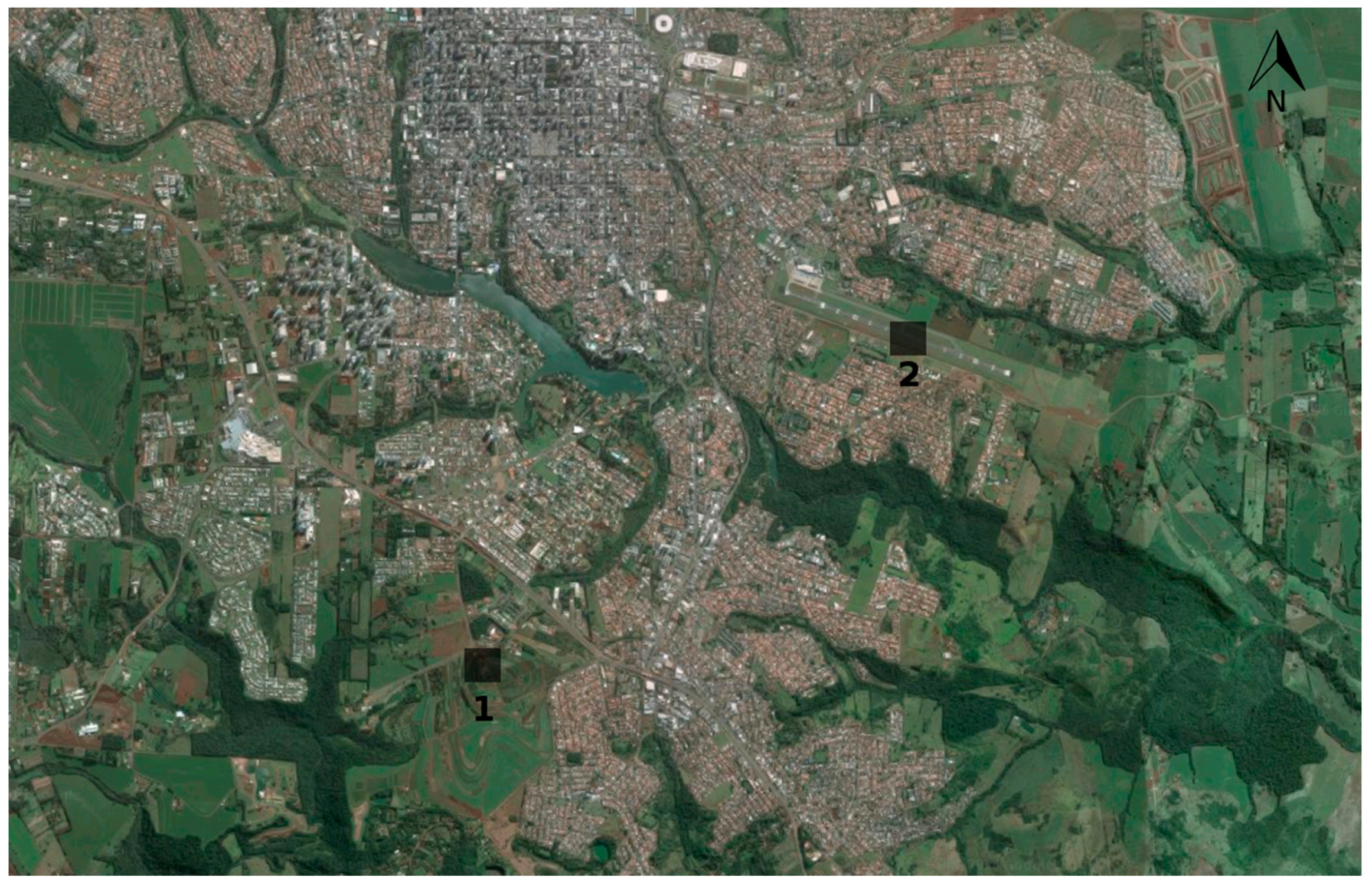
2. Experiments
2.1. Future Scenarios
2.2. Numerical Modeling and Configuration
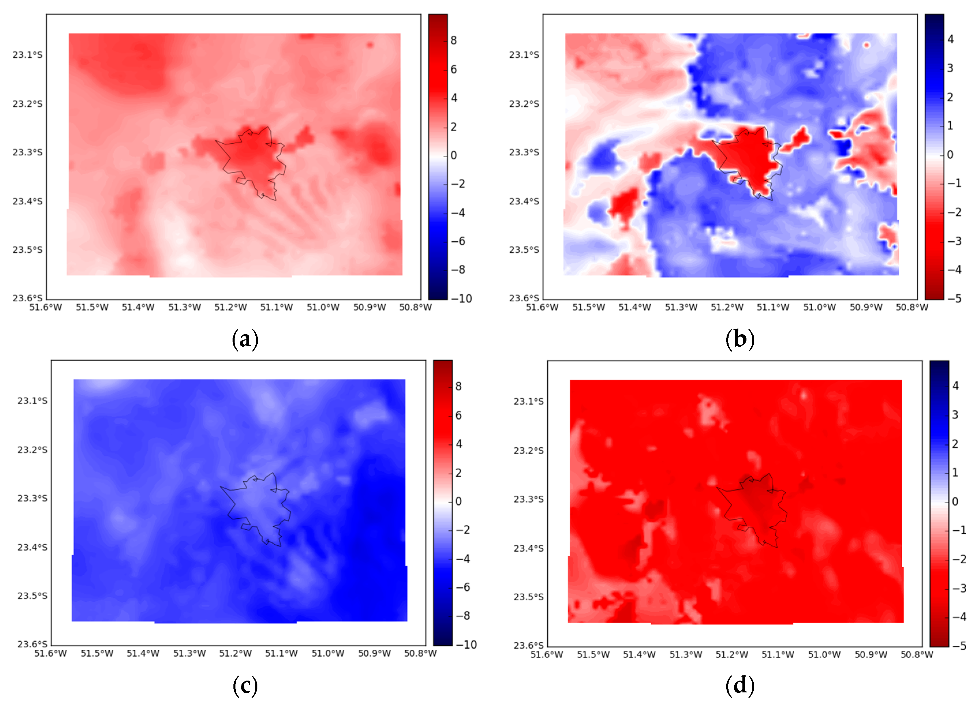
3. Results
4. Discussion and Conclusions
Author Contributions
Acknowledgments
Conflicts of Interest
Abbreviations
| 1. UHI | 2. Urban Heat Island |
| 3. WRF | 4. Weather Research and Forecast |
| 5. GFS | 6. Global Forecast System |
| 7. CCSM3 | 8. Community Climate System Model Version 3 |
| 9. IPCC | 10. Intergovernmental Panel on Climate Change |
| 11. SRES | 12. Special Report of Emission Scenarios |
| 13. SIMEPAR | 14. Meteorological System of Paraná (Sistema Meteorológico do Paraná, in portuguese) |
| 15. SO2 | 16. Sulfur dioxide |
| 17. CO | 18. Carbon monoxide |
| 19. NOx | 20. Nitrogen oxides |
| 21. NMHC | 22. Non-methane hydrocarbons |
| 23. SRESA2 | 24. Simulation with A2 scenario from CCSM3 |
| 25. SRESB1 | 26. Simulation with B1 scenario from CCSM3 |
References
- Intergovernmental Panel on Climate Change (IPCC). Climate Change 2007: The Physical Science Basis, Contribution of Working Group I. In Fourth Assessment Report of the Intergovernmental Panel on Climate Change; Cambridge University Press: Cambridge, UK; New York, NY, USA, 2007; 996p. [Google Scholar]
- Revi, A.; Satterthwaite, D.E.; Aragón-Durand, F.; Corfee-Morlot, J.; Kiunsi, R.B.R.; Pelling, M.; Roberts, D.C.; Solecki, W.; da Silva, J.; Dodman, D.; et al. Urban areas. In Climate Change 2014: Impacts, Adaptation, and Vulnerability. Part A: Global and Sectoral Aspects. Contribution of Working Group II to the Fifth Assessment Report of the Intergovernmental Panel on Climate Change; Field, C.B., Barros, V.R., Dokken, D.J., Mach, K.J., Mastrandrea, M.D., Bilir, T.E., Chatterjee, M., Ebi, K.L., Estrada, Y.O., Genova, R.C., et al., Eds.; Cambridge University Press: Cambridge, UK; New York, NY, USA, 2015; pp. 535–612. [Google Scholar]
- Ribeiro, W.C. Impact of the climate changes in the cities of Brazil (Impacto das mudanças climáticas em cidades no Brasil). Parcer. Estratég. 2008, 27, 293–321. (In Portuguese) [Google Scholar]
- Rosenzweig, C.; Solecki, W.; Hammer, S.A.; Mehrotra, S. Cities lead the way in climate-change action. Nature 2010, 467, 909–911. [Google Scholar] [CrossRef] [PubMed]
- Nakicenovic, N.; Alcamo, J.; Davis, G.; Vries, B.; Fenhann, J.; Gaffin, S.; Kermeth, G.; Amulf, G.; Jung, T.Y.; Kram, T.; et al. Special Report on Emission Scenarios, Published for the Intergovernamental Panel on Climate Change; Cambridge University Press: New York, NY, USA, 2000; 608p. [Google Scholar]
- Früh, B.; Becker, P.; Deutschlander, T.; Hessel, J.D.; Kossman, M.; Mieskes, I.; Namyslo, J.; Roos, M.; Sievers, U.; Steigerwald, T.; et al. Estimation of Climate-Change Impacts on the Urban Heat Load Using an Urban Climate Model and Regional Climate Projections. J. Appl. Meteorol. 2011, 50, 167–184. [Google Scholar] [CrossRef]
- Hamdi, R.; Giot, O.; De Troch, R.; Deckmyn, A.; Termonia, P. Future Climate of Brussels and Paris for the 2050s under A1B scenario. Urban Clim. 2015, 12, 160–182. [Google Scholar] [CrossRef]
- Parker, A.S.; Kusaka, H.; Yamagata, Y. Assessment of the Impact of Metropolitan-Scale Urban Planning Scenarios on the Moist Thermal Environment under Global Warming: A Study of the Tokyo Metropolitan Area Using Regional Climate Modeling. Adv. Meteorol. 2015, 2015, 693754. [Google Scholar]
- Lemonsu, A.; Viguié, V.; Daniel, M.; Masson, V. Vulnerability to heat waves: Impact of urban expansion scenarios on urban heat island and heat stress in Paris (France). Urban Clim. 2015, 14, 586–605. [Google Scholar] [CrossRef]
- Semenza, J.C.; Mccullough, J.; Flanders, W.D.; Mcgeehin, M.A.; Rubin, C.H.; Lumpkin, J.R. Excess hospital admissions during the 1995 heat wave in Chicago. Am. J. Prev. Med. 1999, 16, 269–277. [Google Scholar] [CrossRef]
- Kalnay, E.; Cai, M. Impact of urbanization and land-use change on climate. Nature 2003, 423, 528–531. [Google Scholar] [CrossRef]
- Oke, T.R. Boundary Layer Climates, 2nd ed.; Cambridge University Press: New York, NY, USA, 1988; 435p. [Google Scholar]
- Arnfield, A.J. Two decades of Urban Climate Research: A review of Turbulence Exchanges of Energy and Water, and the Urban Heat Island. Int. J. Climatol. 2003, 23, 1–26. [Google Scholar] [CrossRef]
- Atkinson, B.W. Numerical Modelling of Urban Heat-Island Intensity. Bound. Layer Meteorol. 2003, 109, 285–310. [Google Scholar] [CrossRef]
- Montálvez, J.P.; Rodriguéz, A.; Jiménez, J.I. A study of the urban heat island of Granada. Int. J. Climatol. 2000, 20, 899–911. [Google Scholar] [CrossRef]
- Morris, C.J.G.; Simmonds, I. Associations between varying magnitudes of the urban heat island and the synoptic climatology in Melbourne, Australia. Int. J. Climatol. 2000, 20, 1931–1954. [Google Scholar] [CrossRef]
- Li, D.; Bou-Zeid, E. Synergistic interactions between urban heat islands and heat waves: The impact in cities is larger than the sum of its parts. J. Appl. Meteorol. 2013, 52, 2051–2064. [Google Scholar] [CrossRef]
- Dabbert, W.F.; Hales, J.; Zubrick, S.; Crook, A.; Mueller, C.; Krajewski, W.; Doran, J.C.; Mueller, C.; King, C.; Keener, R.N.; et al. Forecast Issues in the Urban Zone: Report of the 10th Prospectus Development Team of the U.S. Weather Research Program. Bull. Am. Meteorol. Soc. 2000, 81, 2047–2064. [Google Scholar] [CrossRef]
- Freitas, E.D. Circulações Locais em São Paulo e sua Influência na Dispersão de Poluentes. 157 f. Ph.D. Thesis, Atmospheric Science Department, University of São Paulo, São Paulo, Brazil, 2003. [Google Scholar]
- Ketzel, M.; Berkowicz, R.; Muller, W.; Lohmeyer, A. Dependence of street canyon concentrations on above roof wind speed—Implications for numerical modelling. Int. J. Environ. Pollut. 2002, 17, 356–366. [Google Scholar] [CrossRef]
- Urbina Guerrero, V.V. Características das Circulações Locais em Regiões Metropolitanas do Chile Central. 113 f. Master’s Thesis, Instituto de Astronomia, Geofísica e Ciências Atmosféricas, Universidade de São Paulo, São Paulo, Brazil, 2010. [Google Scholar]
- Britter, R.; Hanna, S.R. Flow and dispersion in urban areas. Annu. Rev. Fluid Mech. 2003, 35, 469–496. [Google Scholar] [CrossRef]
- Harman, I.N. The Energy Balance of Urban Areas. 157 f. Ph.D. Thesis, University of Reading, London, UK, 2003. [Google Scholar]
- Marengo, J.A.; Ambrizzi, T. Use of regional climate models in impacts assessments and adaptations studies from continental to regional and local scales: The CREAS (Regional Climate Change Scenarios for South America) initiative in South America. In Proceedings of the 8th International Conference on Southern Hemisphere Meteorology and Oceanography (ICSHMO), Foz do Iguaçu, Brazil, 24–28 April 2006; pp. 291–296. [Google Scholar]
- Marengo, J.A.; Jones, R.; Alves, L.M.; Valverde, M.C. Future change of temperature and precipitation extremes in South America as derived from the PRECIS regional climate modeling system. Int. J. Climatol. 2009, 29, 2241–2255. [Google Scholar] [CrossRef]
- Reboita, M.S.; Rocha, R.P.; Dias, C.G.; Ynoue, R.Y. Climate Projections for South America: RegCM3 Driven by HadCM3 and ECHAM5. Adv. Meteorol. 2014, 2014, 376738. [Google Scholar] [CrossRef]
- IBGE 2014: Data of South and Southeast Region of Brazil. Available online: http://www.ibge.gov.br/ (accessed on 12 May 2017).
- Capucim, M.N.; Brand, V.S.; Machado, C.B.; Martins, L.D.; Allasia, D.G.; Homann, C.T.; Freitas, E.D.; Silva Dias, M.A.F.; Andrade, M.F.; Martins, J.A. South America land use and land cover assessment and preliminary analysis of their impacts on regional atmospheric modeling studies. IEEE J. Sel. Top.Appl. 2014, 8, 1185–1198. [Google Scholar] [CrossRef]
- Skamarock, W.C.; Klemp, J.B.; Dudhia, J.; Gill, D.O.; Barker, D.M.; Duda, M.G.; Huang, X.Y.; Wang, W.; Powers, J.G. A Description of the Advanced Research WRF Version 3; NCAR Technical Note; NCAR/TN-475+STR: Boulder, CO, USA, 2008. [Google Scholar]
- Collins, W.D.; Bitz, C.M.; Blackmon, M.L.; Bonan, G.B.; Bretherton, C.S.; Carton, J.A.; Chang, P.; Doney, S.C.; Hack, J.J.; Henderson, T.B.; et al. The Community Climate System Model Version 3 (CCSM3). J. Clim. 2006, 19, 2122–2143. [Google Scholar] [CrossRef]
- Collins, W.D.; Rasch, P.J.; Boville, B.A.J.; McCaa, J.R.; Williamson, D.L.; Kiehl, J.T.; Briegleb, B.; Bitz, C.; Lin, S.J. Description of the NCAR Community Atmosphere Model (CAM3); NCAR Technical Note; NCAR/TN-464_STR: Boulder, CO, USA, 2004. [Google Scholar]
- Oleson, K.; Dai, Y.; Bonan, G.B.; Bosilovichm, M.; Dickinson, R.; Dirmeyer, P.; Hoffman, F.; Houser, P.; Levis, S.; Niu, G.Y.; et al. Technical Description of the Community Land Model (CLM); NCAR Technical Report; NCAR/TN-461+STR: Boulder, CO, USA, 2004. [Google Scholar]
- Dickinson, R.E.; Oleson, K.W.; Bonan, G.; Hoffman, F.; Thornton, P.; Vertenstein, M.; Yang, Z.L.; Zeng, X. The Community Land Model and its climate statistics as a component of the Community Climate System Model. J. Clim. 2006, 19, 2302–2324. [Google Scholar] [CrossRef]
- Briegleb, B.P.; Bitz, C.M.; Hunke, E.C.; Lipscomb, W.H.; Holland, M.M.; Schramm, J.L.; Moritz, R.E. Scientific Description of the Sea Ice Component in the Community Climate System Model, Version Three. NCAR Technical Report; NCAR/TN-463STR: Boulder, CO, USA, 2004. [Google Scholar]
- Smith, R.D.; Gent, P.R. Reference Manual for the Parallel Ocean Program (POP), Ocean Component of the Community Climate System Model (CCSM2.0 and 3.0). NCAR Technical Report; LA-UR-02-2484: Boulder, CO, USA, 2002. [Google Scholar]
- Mazzoli, C.R. Estudo Numérico da Influência das Mudanças Climáticas e das Emissões Urbanas no Ozônio Troposférico da Região Metropolitana de São Paulo. 162 f. Ph.D. Thesis, University of São Paulo, São Paulo, Brazil, 2003. [Google Scholar]
- Kanamitsu, M.; Alpert, J.C.; Campana, K.A.; Caplan, P.M.; Deaven, D.G.; Iredell, M.; Katz, B.; Pan, H.L.; Sela, J.; White, G.H. Recent changes implemented into the global forecast system at NMC. Weather Forecast. 1991, 6, 425–436. [Google Scholar] [CrossRef]
- Daley, R. Atmospheric Data Analysis; Cambridge Press: New York, NY, USA, 1991; pp. 1–457. [Google Scholar]
- Schneider, A.; Friedl, M.A.; Potere, D. A new map of global urban extent from MODIS data. Environ. Res. Lett. 2009, 4, 044003. [Google Scholar] [CrossRef]
- Kessler, E. On the Distribution and Continuity of Water Substance in Atmospheric Circulation; American Meteorological Society: Boston, MA, USA, 1969; Volume 10, 88p. [Google Scholar]
- Grell, G.A.; Freitas, S.R. A scale and aerosol aware stochastic convective parameterization for weather and air quality modeling. Atmos. Chem. Phys. 2014, 14, 5233–5250. [Google Scholar] [CrossRef]
- Zhang, D.; Anthes, R.A. A High-Resolution Model of the Planetary Boundary Layer—Sensitivity Tests and Comparisons with SESAME-79 Data. J. App. Meteorol. 1982, 21, 1594–1609. [Google Scholar] [CrossRef]
- Chen, F.; Dudhia, J. Coupling an advanced land surface-hydrology model with the Penn State-NCAR MM5 modeling system. Part I: Model implementation and sensitivity. Mon. Weather Rev. 2001, 129, 569–585. [Google Scholar] [CrossRef]
- Kusaka, H.; Kimura, F. Coupling a single-layer urban canopy model with a simple atmospheric model: Impact on urban heat island simulation for an idealized case. J. Meteorol. Soc. Jpn 2004, 82, 67–80. [Google Scholar] [CrossRef]
- Hong, S.; Noh, Y.; Dudhia, J. A new vertical diffusion package with explicit treatment of entrainment processes. Mon. Weather Rev. 2006, 134, 2318–2341. [Google Scholar] [CrossRef]
- Dudhia, J. Numerical Study of Convection Observed during the Winter Monsoon Experiment Using a Mesoscale Two—Dimensional Model. J. Atmos. Sci. 1989, 46, 3077–3107. [Google Scholar] [CrossRef]
- Mlawer, E.J.; Taubman, S.J.; Brown, P.D.; Iacono, M.J.; Clough, S. A Radiative transfer for inhomogeneous atmospheres: RRTM, a validated correlated-k model for the longwave. J. Geophys. Res. Atmos. 1997, 102, 16663–16682. [Google Scholar] [CrossRef]
- Taylor, K.E. Summarizing multiple aspects of model performance in a single diagram. J. Geophys. Res. 2001, 106, 7183–7192. [Google Scholar] [CrossRef]


Publisher’s Note: MDPI stays neutral with regard to jurisdictional claims in published maps and institutional affiliations. |
© 2017 by the authors. Licensee MDPI, Basel, Switzerland. This article is an open access article distributed under the terms and conditions of the Creative Commons Attribution (CC BY) license (https://creativecommons.org/licenses/by/4.0/).
Share and Cite
Morais, M.V.B.d.; Guerrero, V.V.U.; Martins, L.D.; Martins, J.A. Dynamical Downscaling of Future Climate Change Scenarios in Urban Heat Island and Its Neighborhood in a Brazilian Subtropical Area. Proceedings 2017, 1, 106. https://doi.org/10.3390/ecas2017-04130
Morais MVBd, Guerrero VVU, Martins LD, Martins JA. Dynamical Downscaling of Future Climate Change Scenarios in Urban Heat Island and Its Neighborhood in a Brazilian Subtropical Area. Proceedings. 2017; 1(5):106. https://doi.org/10.3390/ecas2017-04130
Chicago/Turabian StyleMorais, Marcos Vinicius Bueno de, Viviana Vanesa Urbina Guerrero, Leila Droprinchinski Martins, and Jorge Alberto Martins. 2017. "Dynamical Downscaling of Future Climate Change Scenarios in Urban Heat Island and Its Neighborhood in a Brazilian Subtropical Area" Proceedings 1, no. 5: 106. https://doi.org/10.3390/ecas2017-04130