Sensitivity Assessment of WRF Parameterizations over Europe ^†

Abstract

Evaluation of the performance of the parameterization schemes used in the WRF model is assessed for temperature and precipitation over Europe at 36 km by 36 km grid resolution using gridded data from the ECA & D 0.25° regular grid. Simulations are performed for a winter (i.e., January 2015) and a summer (i.e., July 2015) month using the two way nesting approach. A step-wise decision approach is followed, beginning with 18 simulations for the various microphysics schemes followed by 45 more, concerning all of the model’s PBL, Cumulus, Long-wave, Short-wave and Land Surface schemes. The best performing scheme at each step is chosen by integrating the entropy weighting method ‘Technique for Order Performance by Similarity to Ideal Solution’ (TOPSIS). The concluding scheme set consists of the Mansell-Ziegler-Bruning microphysics scheme, the Bougeault-Lacarrere PBL scheme, the Kain-Fritsch cumulus scheme, the RRTMG scheme for short-wave, the New Goddard for long-wave radiation and a seasonal-variable sensitive option for the Land Surface scheme.

1. Introduction

The Advanced Research Weather Research and Forecasting model (ARW-WRF, hereafter WRF) [1] is a nonhydrostatic mesoscale numerical weather prediction system, that includes a wide range of physical parameterizations and it can be initialized either by data from a GCM or by reanalysis data. It is an ideal tool for studying phenomena that require high spatial resolution. WRF applications only use a single set of parameterization schemes due to the computational cost of running all possible combinations. Choosing the best performing set of parameterizations is challenging because their performance is highly spatial and time dependent. A significant number of studies have been conducted, exploring WRF sensitivity to different parameterization schemes e.g., [2,3,4,5,6].

Mooney et al. [2] evaluated the sensitivity of WRF to several parameterization schemes for regional climates of Europe over the period 1990–1995. Their results for temperature show a significant dependence on the land surface model, while averaged daily precipitation levels appear to be relatively insensitive to the longwave radiation scheme chosen. They conclude that modelling precipitation is problematic for WRF with biases of up to 100%. Borge et al. [3] studied WRF sensitivity over the Iberian Peninsula for two 1-week periods in the winter and summer of 2005. Their findings suggest that no particular scheme or option produces the best results for all the statistical parameters and/or geographical locations examined. The optimum configuration they provided for the model is based on aggregated performance. Bukovsky and Karoly [4] examined how different land surface models and cumulus schemes affect precipitation over North America for May, June, July, and August over the period 1991–1995. Their results showed that precipitation was sensitive to the choice of land surface model and cumulus scheme, emphasizing the importance of testing WRF output for sensitivity to parameterizations for regional climate modelling applications. Jin et al. [5] also presented a sensitivity study of four land surface schemes in the WRF model over the western US. Their simulation period covered a year from 1 October 1995 to 30 September 1996, resulting in acknowledging the strong effect that land surface processes have on temperature and their poor effect on precipitation which is overestimated by the model. Flaounas et al. [6] examined how convection and planetary boundary layer (PBL) parameterization affect the sensitivity of WRF in a study of the 2006 West African monsoon. Their results show that PBL schemes have the strongest effect on the vertical distribution of temperature, humidity, and rainfall amount, whereas precipitation variability is particularly sensitive to convection parameterization schemes.

The objective of this study is to assess the sensitivity of WRF parameterizations over Europe at a 36 × 36 km grid cell resolution and produce a final parameterization combination that performs best for the whole European region. The long term purpose of this study is to calibrate the RCM to its best possible performing set up in order to be used for downscaling GCM data.

2. Method

2.1. Modelling Domains and Initialization

The Weather Research and Forecasting (WRF) [1] version 3.7.1 is used, here, to dynamically downscale the ENSEMBLES daily gridded observational dataset (E-OBS) [7,8] in a nesting approach over Europe in order to assess the model’s sensitivity to different parameterization set ups by examining its ability to reproduce spatial patterns of the mean temperature and precipitation over Europe. Due to the computationally prohibitive nature of running WRF the simulations are performed for a winter and a summer month (i.e., January and July 2015). The dynamical downscaling approach is following the two way nesting approach with grid resolutions of 108 km and 36 km with the finer nested domain covering the European region (Figure 1).

The initial set of simulations concerned the Microphysics parameterization schemes with all other parameterizations at their default values. The second simulation group explored the effect of the PBL schemes since it has no direct interactions with microphysics [9] (Figure 2), followed by the Cumulus parameterizations which do not interact with PBL, the Longwave and Shortwave radiation schemes being independent of the previous ones and finally Land Surface schemes. Our simulation groups include most of the existing options the WRF model can offer. Any options that are not included in this study were either extremely time consuming, not being able to run with the model’s multi-core mode, or did not produce an hourly output so they were excluded on the basis of not being on the same time scale with the rest.

At the end of each simulation group, statistical measures for model’s performance were calculated (

Table 1. Statistical measures representing each simulation.

Measure	Formula
Mean bias	$\frac{{{\displaystyle \sum }}_{i=1}^n\left(X_{predicted}-X_{observed}\right)}{n}$
Root square error	$\sqrt{\frac{{{\displaystyle \sum }}_{i=1}^n{\left(X_{predicted}-X_{observed}\right)}^2}{n}}$
Index of agreement	$1-\frac{{{\displaystyle \sum }}_{i=1}^n{\left(X_{predicted}-X_{observed}\right)}^2}{{{\displaystyle \sum }}_{i=1}^n{\left(\left|X_{predicted}-{\overline{X}}_{observed}\right|+\left|X_{observed}-{\overline{X}}_{observed}\right|\right)}^2}$
Mean absolute error	$\frac{{{\displaystyle \sum }}_{i=1}^n\left|X_{predicted}-X_{observed}\right|}{n}$

) as well as a spatial distribution map of the mean bias was created. The estimation of these measures was conducted by comparison of the model’s mean daily output to the E-OBS dataset from the EU-FP6 project ENSEMBLES provided by the ECA & D project for every grid cell (http://www.ecad.eu).

In order to identify the best parameterization option for each simulation group the TOPSIS (Technique for Order Preference by Similarity to the Ideal Solution) method was utilized. It is a multi-criteria decision analysis method summarized below. Our decision making approach focused on mean temperature prediction, being the variable best forecasted by numeric models and additionally, the effects of our scheme choices on precipitation were also assessed.

2.2. Technique for Order Preference by Similarity to the Ideal Solution

The TOPSIS method was first developed by Hwang and Yoon [10] with further developments by Yoon [11] and Hwang et al. [12]. It ranks the alternatives according to their distances from the ideal and the negative ideal solution, i.e., the best alternative has simultaneously the shortest distance from the ideal solution and the farthest distance from the negative ideal solution. Some of the advantages of TOPSIS methods are: simplicity, rationality, comprehensibility, good computational efficiency and ability to measure the relative performance for each alternative in a simple mathematical form. TOPSIS is a method of compensatory aggregation that compares a set of alternatives by identifying weights for each criterion, normalizing scores for each criterion and calculating the geometric distance between each alternative and the ideal alternative, which is the best score in each criterion. The TOPSIS process is carried out as follows:

Step 1:

Creating an evaluation matrix consisting of m alternatives and n criteria.

Step 2:

Normalizing the evaluation matrix.

Step 3:

Calculating a weighted normalized decision matrix by determining the weights of the various factors. In this study Shannon’s entropy theory [13] was adopted in order to calculate the weighting factors.

Step 4:

Determining the positive-ideal solution (PIS) and the negative-ideal solution (NIS) by defining each of the criteria in use as positive or negative.

Step 5:

Calculating the distance between the target alternative and (PIS) and the distance between the target alternative and (NIS).

Step 6:

Calculating the Closeness Coefficient (CC) of each alternative. The coefficient is defined to determine the ranking order of each alternative.

Step 7:

Determining the ranking order of all alternatives according to the closeness to the ideal solution which is based on the criteria we have inserted in the method and selecting the best or the worst one from the set of feasible alternatives.

3. Results and Discussion

Τhe various options of Microphysics parameterization schemes were assessed firstly keeping all other model options at their default values. The statistical measures were calculated for each simulation and were used as input for the multi-criteria ranking method. The TOPSIS ranking results as well as the statistical measures are shown in

Table 2. Statistical measures and TOPSIS ranking for the Microphysics simulation group.

Option	Microphysics Scheme	Mean Bias				Root Square Error				Index of Agreement				Mean Absolute Error				TOPSIS Ranking
		Temp		Prec		Temp		Prec		Temp		Prec		Temp		Prec		Temp		Prec
		JAN	JUL	JAN	JUL	JAN	JUL	JAN	JUL	JAN	JUL	JAN	JUL	JAN	JUL	JAN	JUL	JAN	JUL	JAN	JUL
1	Kessler Scheme [15]	−0.41	−1.40	−0.51	−0.37	2.69	2.19	3.54	3.86	0.97	0.97	0.79	0.71	1.98	1.77	1.56	1.81	16	17	17	17
2	Lin et al. Scheme [16]	−0.40	−1.03	0.12	−0.02	2.61	1.93	3.72	3.95	0.97	0.97	0.80	0.73	1.91	1.51	1.68	1.87	15	8	9	2
3	WSM3 Single-moment 3-class Scheme [17]	−0.87	−1.20	0.09	−0.09	2.74	2.01	3.65	3.78	0.96	0.97	0.80	0.74	2.11	1.60	1.66	1.82	17	15	8	4
4	WSM5 Single-moment 5-class Scheme [17]	−0.25	−1.20	0.13	−0.10	2.61	2.01	3.62	3.82	0.97	0.97	0.81	0.74	1.89	1.60	1.67	1.82	12	16	10	6
6	WSM6 Single-moment 6-class Scheme [18]	−0.25	−1.07	0.13	−0.09	2.61	1.95	3.64	3.83	0.97	0.97	0.81	0.73	1.89	1.53	1.68	1.82	7	10	11	5
7	Goddard Scheme [19]	−0.21	−1.12	0.07	−0.11	2.61	1.99	3.48	3.82	0.97	0.97	0.81	0.73	1.88	1.57	1.61	1.81	5	13	7	7
8	Thompson Scheme [20]	−0.24	−0.89	−0.04	0.16	2.61	1.87	3.44	3.95	0.97	0.98	0.81	0.72	1.89	1.43	1.58	1.94	6	6	6	14
9	Milbrandt-Yau Double Moment Scheme [21,22]	−0.25	−0.93	0.19	0.17	2.61	1.89	3.51	4.00	0.97	0.97	0.82	0.72	1.90	1.46	1.66	1.95	18	7	14	16
10	Morrison 2-moment Scheme [23]	−0.25	−1.06	−0.02	−0.13	2.62	1.94	3.46	3.79	0.97	0.97	0.81	0.73	1.90	1.52	1.59	1.80	10	9	4	13
11	CAM V5.1 2-moment 5-class Scheme [24]	−0.02	−1.42	−0.26	−0.54	2.56	2.18	3.62	3.49	0.97	0.97	0.78	0.73	1.81	1.78	1.58	1.65	1	18	18	18
13	SBU Stony–Brook University Scheme [25]	−0.16	−0.87	0.03	0.02	2.59	1.86	3.40	3.85	0.97	0.97	0.81	0.73	1.86	1.43	1.59	1.86	2	5	5	1
14	WDM5 Double Moment 5-class Scheme [26]	−0.25	−1.10	0.15	−0.11	2.60	1.97	3.66	3.82	0.97	0.97	0.80	0.73	1.88	1.54	1.70	1.83	9	11	12	8
16	WDM6 Double Moment 6-class Scheme [26]	−0.25	−1.10	0.16	−0.13	2.60	1.97	3.70	3.82	0.97	0.97	0.80	0.73	1.88	1.55	1.71	1.82	8	12	13	12
17	NSSL 2–moment Scheme [14]	−0.17	−0.83	−0.03	0.12	2.59	1.83	3.36	3.83	0.97	0.98	0.81	0.73	1.86	1.40	1.56	1.91	3	1	2	10
18	NSSL 2-moment Scheme with CCN Prediction [14]	−0.17	−0.83	−0.03	0.11	2.59	1.83	3.36	3.83	0.97	0.98	0.81	0.73	1.86	1.40	1.56	1.91	4	3	1	9
19	NSSL 1-moment 7-class Scheme	−0.31	−0.83	−0.25	0.12	2.62	1.83	3.44	3.83	0.97	0.98	0.81	0.73	1.91	1.40	1.57	1.91	13	2	15	11
21	NSSL 1-moment 6-class Scheme [27]	−0.31	−1.13	−0.25	−0.06	2.62	1.99	3.47	3.94	0.97	0.97	0.81	0.71	1.91	1.57	1.58	1.86	14	14	16	3
28	Aerosol-aware Thompson Scheme [28]	−0.25	−0.84	−0.02	0.17	2.60	1.84	3.46	3.95	0.97	0.98	0.81	0.72	1.89	1.41	1.58	1.95	11	4	3	15

. Option 17,the NSSL 2-moment Scheme [14], has been chosen as the best Microphysics parameterization scheme: it is ranking 1st for temperature in July and 3rd for temperature in January. However, the two better schemes for temperature in January (i.e., CAM V5.1 2-moment 5-class Scheme and SBU Stony—Brook University Scheme) are not so good for temperature in July. In addition, option 17 presents one of the best performances for predicting mean precipitation for January. However, the selected scheme is not one of the best for predicting precipitation in July since this month has very low and location dependant precipitation rates in Europe. The NSSL 2-mom is a double moment scheme for cloud droplets, rain drops, ice crystals, snow, graupel, and hail, which has one prediction equation for mass mixing ratio (kg/kg) per species (Qrain, Qsnow, etc.) and a prediction equation for number concentration (#/kg) per species (Nrain, Nsnow, etc.).

With the Microphysics option set to 17 we conducted the second set of simulations, assessing the PBL options provided by the WRF model. PBL options only work with certain Surface Layer options in the model so there were specific combinations of PBL/Surface Layer schemes to be used as presented in Table 3. A PBL scheme’s purpose is to distribute surface fluxes with boundary layer eddy fluxes and allow for PBL growth by entrainment. There are 2 classes of PBL schemes

-

Turbulent kinetic energy prediction (Mellor-Yamada-Janjic, MYNN, Bougeault-Lacarrere, TEMF, QNSE, CAM UW)

-

Diagnostic non-local (YSU, GFS, MRF, ACM2)

The Surface Layer schemes use similarity theory to determine exchange coefficients and diagnostics of 2 m temperature. Moisture and 10 m winds. They provide the exchange coefficient to the land-surface models, the friction velocity to the PBL scheme and surface fluxes over water points. These schemes have variations in their stability functions and roughness lengths. Τhe best performing options for temperature was option 8 for PBL which corresponds to the Bougeault-Lacarrere Scheme [29] in combination with option 1 meaning the MM5 Similarity [30] Surface Layer scheme. However, these options are not the best for precipitation. The Bougeault-Lacarrere Scheme is a turbulent kinetic energy (TKE) prediction scheme while the MM5 Similarity is based on Monin-Obukhov with Carslon-Boland viscous sub-layer and standard similarity functions.

The next simulation group focused on the Cumulus parameterization schemes shown in Table 4. Convective parameterization schemes were designed to reduce atmospheric instability in the model. Prediction of precipitation is actually just a by-product of the way in which a scheme does this. Consequently, these schemes may not predict the location and timing of convective precipitation as well as we might expect. For climate models, the location and timing of precipitation is less important than for weather forecast models. The scheme that performed best for temperatures were the model’s default Kain-Fritsch Scheme [31] (option 1) as well as the OSAS Old Simplified Arakawa-Schubert [32] (option 4). We decided to keep the model’s default Kain-Fritsch Scheme (option 1) for the next simulation group since it is better for winter precipitation, as well. The Kain-Fritsch Scheme is a deep and shallow convection sub-grid scheme using a mass flux approach with downdrafts and CAPE removal time scale. It includes cloud, rain, ice and snow detrainment.

Longwave radiation schemes were the simulation group that followed. These schemes compute clear-sky and cloud upward and downward radiation fluxes and they consider IR emission from layers. Surface emissivity is based on land-type and flux divergence leads to cooling in a layer while downward flux at the surface is important in the land energy budget. IR radiation generally leads to cooling in clear air (~2 K/day), stronger cooling at cloud tops and warming at cloud base. The options provided by the model are shown in Table 5. Looking at the ranking of the simulations that took place, the RRTMG Fast version Longwave Scheme [33] (option 24) had the top ranking in predicting mean temperature for both January and July and a relatively high ranking concerning precipitation in January. The RRTMG scheme is actually a new version of Rapid Radiative Transfer Model including the Monte Carlo Independent Column Approximation (MCICA) [34] method of random cloud overlap.

The Shortwave radiation schemes simulation group was assessed next according to the options of Table 6. They compute clear sky and cloudy solar fluxes, including the annual and diurnal solar cycle. Most of them consider downward and upward (reflected) fluxes (Dudhia scheme only has downward flux). They consider primarily a warming effect in clear sky and they are a very important component of surface energy balance. The New Goddard Shortwave Scheme [35] (option 5) is one of the best schemes for simulating temperature for both months. However, this scheme is not among the best schemes for precipitation prediction.

Table 3. Statistical measures and TOPSIS ranking for the PBL/Surface Layer simulation group.

Option	PBL/Surface Layer Scheme	Mean Bias				Root Square Error				Index of Agreement				Mean Absolute Error				TOPSIS Ranking
		Temp		Prec		Temp		Prec		Temp		Prec		Temp		Prec		Temp		Prec
		JAN	JUL	JAN	JUL	JAN	JUL	JAN	JUL	JAN	JUL	JAN	JUL	JAN	JUL	JAN	JUL	JAN	JUL	JAN	JUL
1/1	YSU/MM5 Yonsei University Scheme [36]/MM5 [30]	0.17	0.83	0.03	−0.12	2.59	1.83	3.36	3.83	0.97	0.98	0.81	0.73	1.86	1.40	1.56	1.91	2	2	2	6
2/2	MYJ/Eta Mellor-Yamada-Janjic Scheme [37]/Eta [38]	0.33	1.27	0.09	−0.62	2.61	2.13	3.38	4.00	0.97	0.97	0.80	0.72	1.90	1.67	1.56	2.15	11	11	8	13
4/4	QNSE/QNSE Quasi-normal Scale Elimination Scheme [39]	0.41	1.92	−0.03	−0.67	2.63	2.60	3.48	4.26	0.97	0.95	0.80	0.70	1.94	2.14	1.62	2.26	14	18	6	14
5/1	MYNN2/MM5 Mellor-Yamada Nakanishi Niino Level 2.5 [40]/[30]	0.36	0.93	0.11	−0.20	2.63	1.90	3.36	3.77	0.97	0.97	0.80	0.73	1.93	1.46	1.56	1.91	12	5	11	4
5/2	MYNN2/Eta [40]/[38]	0.85	1.58	0.22	−0.28	2.86	2.48	10.11	5.94	0.96	0.96	0.29	0.51	2.15	1.92	2.43	2.22	18	16	18	16
5/5	MYNN2/MYNN [40]	0.29	1.51	0.11	−0.44	2.63	2.28	3.35	3.87	0.97	0.96	0.81	0.73	1.91	1.81	1.56	2.04	8	12	12	10
6/1	MYNN3/MM5 Mellor-Yamada Nakanishi Niino Level 3 [41]/[30]	0.38	0.96	0.10	−0.18	2.63	1.91	3.37	3.82	0.97	0.97	0.80	0.73	1.93	1.47	1.56	1.93	13	7	9	7
6/2	MYNN3/Eta [41]/[38]	0.83	1.56	0.11	−0.28	2.84	2.43	11.46	6.20	0.96	0.96	0.25	0.50	2.13	1.89	2.49	2.25	17	15	17	17
6/5	MYNN3/MYNN [41]	0.31	1.55	0.10	−0.41	2.62	2.29	3.36	3.96	0.97	0.96	0.81	0.72	1.91	1.84	1.56	2.07	9	13	10	12
7/1	ACM2/MM5 Asymmetric Convection Model 2 Scheme [42]/[30]	0.22	1.08	−0.03	0.04	2.59	1.96	3.37	3.77	0.97	0.97	0.81	0.73	1.88	1.54	1.58	1.81	7	9	3	2
7/7	ACM2/Pleim-Xiu [42]/[43]	0.22	1.58	−0.11	−0.26	2.59	2.32	3.48	3.96	0.97	0.96	0.80	0.72	1.88	1.89	1.63	1.97	6	14	13	9
8/1	BouLac/MM5 Bougeault-Lacarrere Scheme [29]/[30]	0.002	0.69	−0.07	−0.28	2.61	1.79	3.40	4.00	0.97	0.98	0.81	0.72	1.85	1.36	1.60	2.02	1	1	7	11
8/2	BouLac/Eta [29]/[38]	0.82	2.08	0.34	−0.03	2.98	3.18	8.60	6.73	0.96	0.93	0.33	0.42	2.22	2.41	2.51	2.35	16	19	19	18
9/1	UW/MM5 University of Washington Scheme [44]/[30]	0.32	0.93	0.12	−0.12	2.59	1.89	3.36	3.73	0.97	0.97	0.80	0.73	1.88	1.45	1.55	1.87	10	6	14	3
9/2	UW/Eta [44]/[38]	0.94	1.68	0.33	−0.13	2.93	2.55	8.75	5.11	0.96	0.95	0.33	0.58	2.20	1.99	2.39	2.15	19	17	16	15
10/10	TEMF/TEMF Surface Layer Scheme [45]	0.65	0.97	−0.77	−3.22	2.77	2.16	4.62	9.81	0.96	0.97	0.73	0.46	2.11	1.67	2.07	4.39	15	10	15	19
11/1	Shin-Hong/MM5 Scale-aware Scheme [46]/[30]	0.20	0.85	0.04	−0.11	2.59	1.85	3.36	3.82	0.97	0.98	0.81	0.73	1.86	1.41	1.56	1.91	5	3	4	5
12/1	GBM/MM5 Grenier-Bretherton-McCaa Scheme [47]/[30]	0.17	0.99	0.05	−0.18	2.57	1.94	3.36	3.85	0.97	0.97	0.81	0.72	1.85	1.49	1.56	1.93	3	8	5	8
99/1	MRF/MM5 [48]/[30]	−0.19	0.86	0.02	0.13	2.67	1.88	3.31	3.64	0.96	0.98	0.81	0.74	1.88	1.45	1.55	1.76	4	4	1	1

Table 3. Statistical measures and TOPSIS ranking for the PBL/Surface Layer simulation group.

Option	PBL/Surface Layer Scheme	Mean Bias				Root Square Error				Index of Agreement				Mean Absolute Error				TOPSIS Ranking
		Temp		Prec		Temp		Prec		Temp		Prec		Temp		Prec		Temp		Prec
		JAN	JUL	JAN	JUL	JAN	JUL	JAN	JUL	JAN	JUL	JAN	JUL	JAN	JUL	JAN	JUL	JAN	JUL	JAN	JUL
1/1	YSU/MM5 Yonsei University Scheme [36]/MM5 [30]	0.17	0.83	0.03	−0.12	2.59	1.83	3.36	3.83	0.97	0.98	0.81	0.73	1.86	1.40	1.56	1.91	2	2	2	6
2/2	MYJ/Eta Mellor-Yamada-Janjic Scheme [37]/Eta [38]	0.33	1.27	0.09	−0.62	2.61	2.13	3.38	4.00	0.97	0.97	0.80	0.72	1.90	1.67	1.56	2.15	11	11	8	13
4/4	QNSE/QNSE Quasi-normal Scale Elimination Scheme [39]	0.41	1.92	−0.03	−0.67	2.63	2.60	3.48	4.26	0.97	0.95	0.80	0.70	1.94	2.14	1.62	2.26	14	18	6	14
5/1	MYNN2/MM5 Mellor-Yamada Nakanishi Niino Level 2.5 [40]/[30]	0.36	0.93	0.11	−0.20	2.63	1.90	3.36	3.77	0.97	0.97	0.80	0.73	1.93	1.46	1.56	1.91	12	5	11	4
5/2	MYNN2/Eta [40]/[38]	0.85	1.58	0.22	−0.28	2.86	2.48	10.11	5.94	0.96	0.96	0.29	0.51	2.15	1.92	2.43	2.22	18	16	18	16
5/5	MYNN2/MYNN [40]	0.29	1.51	0.11	−0.44	2.63	2.28	3.35	3.87	0.97	0.96	0.81	0.73	1.91	1.81	1.56	2.04	8	12	12	10
6/1	MYNN3/MM5 Mellor-Yamada Nakanishi Niino Level 3 [41]/[30]	0.38	0.96	0.10	−0.18	2.63	1.91	3.37	3.82	0.97	0.97	0.80	0.73	1.93	1.47	1.56	1.93	13	7	9	7
6/2	MYNN3/Eta [41]/[38]	0.83	1.56	0.11	−0.28	2.84	2.43	11.46	6.20	0.96	0.96	0.25	0.50	2.13	1.89	2.49	2.25	17	15	17	17
6/5	MYNN3/MYNN [41]	0.31	1.55	0.10	−0.41	2.62	2.29	3.36	3.96	0.97	0.96	0.81	0.72	1.91	1.84	1.56	2.07	9	13	10	12
7/1	ACM2/MM5 Asymmetric Convection Model 2 Scheme [42]/[30]	0.22	1.08	−0.03	0.04	2.59	1.96	3.37	3.77	0.97	0.97	0.81	0.73	1.88	1.54	1.58	1.81	7	9	3	2
7/7	ACM2/Pleim-Xiu [42]/[43]	0.22	1.58	−0.11	−0.26	2.59	2.32	3.48	3.96	0.97	0.96	0.80	0.72	1.88	1.89	1.63	1.97	6	14	13	9
8/1	BouLac/MM5 Bougeault-Lacarrere Scheme [29]/[30]	0.002	0.69	−0.07	−0.28	2.61	1.79	3.40	4.00	0.97	0.98	0.81	0.72	1.85	1.36	1.60	2.02	1	1	7	11
8/2	BouLac/Eta [29]/[38]	0.82	2.08	0.34	−0.03	2.98	3.18	8.60	6.73	0.96	0.93	0.33	0.42	2.22	2.41	2.51	2.35	16	19	19	18
9/1	UW/MM5 University of Washington Scheme [44]/[30]	0.32	0.93	0.12	−0.12	2.59	1.89	3.36	3.73	0.97	0.97	0.80	0.73	1.88	1.45	1.55	1.87	10	6	14	3
9/2	UW/Eta [44]/[38]	0.94	1.68	0.33	−0.13	2.93	2.55	8.75	5.11	0.96	0.95	0.33	0.58	2.20	1.99	2.39	2.15	19	17	16	15
10/10	TEMF/TEMF Surface Layer Scheme [45]	0.65	0.97	−0.77	−3.22	2.77	2.16	4.62	9.81	0.96	0.97	0.73	0.46	2.11	1.67	2.07	4.39	15	10	15	19
11/1	Shin-Hong/MM5 Scale-aware Scheme [46]/[30]	0.20	0.85	0.04	−0.11	2.59	1.85	3.36	3.82	0.97	0.98	0.81	0.73	1.86	1.41	1.56	1.91	5	3	4	5
12/1	GBM/MM5 Grenier-Bretherton-McCaa Scheme [47]/[30]	0.17	0.99	0.05	−0.18	2.57	1.94	3.36	3.85	0.97	0.97	0.81	0.72	1.85	1.49	1.56	1.93	3	8	5	8
99/1	MRF/MM5 [48]/[30]	−0.19	0.86	0.02	0.13	2.67	1.88	3.31	3.64	0.96	0.98	0.81	0.74	1.88	1.45	1.55	1.76	4	4	1	1

Table 4. Statistical measures and TOPSIS ranking for the Cumulus simulation group.

Option	Cumulus Scheme	Mean Bias				Root Square Error				Index of Agreement				Mean Absolute Error				TOPSIS Ranking
		Temp		Prec		Temp		Prec		Temp		Prec		Temp		Prec		Temp		Prec
		JAN	JUL	JAN	JUL	JAN	JUL	JAN	JUL	JAN	JUL	JAN	JUL	JAN	JUL	JAN	JUL	JAN	JUL	JAN	JUL
1	Kain-Fritsch Scheme [31]	0.002	0.691	−0.073	−0.282	2.608	1.791	3.404	4.001	0.966	0.977	0.814	0.715	1.854	1.357	1.595	2.020	3	1	2	7
2	BMJ Betts-Miller-Janjic Scheme [37]	−0.004	0.718	0.007	0.222	2.608	1.801	3.345	3.443	0.966	0.977	0.814	0.753	1.851	1.366	1.571	1.651	8	2	3	5
3	GF Grell-Freitas Ensemble Scheme [49]	0.003	0.902	−0.087	0.166	2.607	1.866	3.427	3.668	0.966	0.975	0.810	0.736	1.849	1.438	1.603	1.728	5	6	7	2
4	OSAS Old Simplified Arakawa-Schubert [32]	−0.001	0.827	0.006	0.335	2.608	1.835	3.338	3.411	0.966	0.976	0.816	0.751	1.850	1.401	1.559	1.611	1	3	6	6
5	G3 Grell 3D Ensemble Scheme [50]	−0.002	0.923	−0.110	0.203	2.608	1.873	3.385	3.530	0.966	0.975	0.817	0.749	1.850	1.446	1.590	1.654	4	8	8	4
6	Tiedtke Scheme [51]	−0.003	0.851	0.011	0.587	2.619	1.839	3.320	3.451	0.965	0.976	0.820	0.742	1.860	1.408	1.544	1.572	7	4	1	10
14	NSAS New Simplified Arakawa-Schubert [52]	−0.008	0.902	−0.152	0.384	2.609	1.865	3.420	3.911	0.966	0.976	0.816	0.698	1.851	1.439	1.616	1.714	9	5	9	8
16	New Tiedtke Scheme [53]	0.046	0.960	0.229	0.514	2.620	1.871	3.269	3.268	0.965	0.975	0.811	0.763	1.865	1.448	1.496	1.544	10	9	10	9
93	GD Grell-Devenyi Ensemble Scheme [50]	−0.001	0.913	0.046	0.171	2.606	1.871	3.383	3.617	0.966	0.975	0.802	0.737	1.849	1.442	1.577	1.721	2	7	5	3
99	old KF Old Kain-Fritsch Scheme [54]	0.003	0.991	−0.038	−0.027	2.604	1.912	3.355	3.731	0.966	0.974	0.814	0.728	1.847	1.478	1.579	1.891	6	10	4	1

Table 4. Statistical measures and TOPSIS ranking for the Cumulus simulation group.

Option	Cumulus Scheme	Mean Bias				Root Square Error				Index of Agreement				Mean Absolute Error				TOPSIS Ranking
		Temp		Prec		Temp		Prec		Temp		Prec		Temp		Prec		Temp		Prec
		JAN	JUL	JAN	JUL	JAN	JUL	JAN	JUL	JAN	JUL	JAN	JUL	JAN	JUL	JAN	JUL	JAN	JUL	JAN	JUL
1	Kain-Fritsch Scheme [31]	0.002	0.691	−0.073	−0.282	2.608	1.791	3.404	4.001	0.966	0.977	0.814	0.715	1.854	1.357	1.595	2.020	3	1	2	7
2	BMJ Betts-Miller-Janjic Scheme [37]	−0.004	0.718	0.007	0.222	2.608	1.801	3.345	3.443	0.966	0.977	0.814	0.753	1.851	1.366	1.571	1.651	8	2	3	5
3	GF Grell-Freitas Ensemble Scheme [49]	0.003	0.902	−0.087	0.166	2.607	1.866	3.427	3.668	0.966	0.975	0.810	0.736	1.849	1.438	1.603	1.728	5	6	7	2
4	OSAS Old Simplified Arakawa-Schubert [32]	−0.001	0.827	0.006	0.335	2.608	1.835	3.338	3.411	0.966	0.976	0.816	0.751	1.850	1.401	1.559	1.611	1	3	6	6
5	G3 Grell 3D Ensemble Scheme [50]	−0.002	0.923	−0.110	0.203	2.608	1.873	3.385	3.530	0.966	0.975	0.817	0.749	1.850	1.446	1.590	1.654	4	8	8	4
6	Tiedtke Scheme [51]	−0.003	0.851	0.011	0.587	2.619	1.839	3.320	3.451	0.965	0.976	0.820	0.742	1.860	1.408	1.544	1.572	7	4	1	10
14	NSAS New Simplified Arakawa-Schubert [52]	−0.008	0.902	−0.152	0.384	2.609	1.865	3.420	3.911	0.966	0.976	0.816	0.698	1.851	1.439	1.616	1.714	9	5	9	8
16	New Tiedtke Scheme [53]	0.046	0.960	0.229	0.514	2.620	1.871	3.269	3.268	0.965	0.975	0.811	0.763	1.865	1.448	1.496	1.544	10	9	10	9
93	GD Grell-Devenyi Ensemble Scheme [50]	−0.001	0.913	0.046	0.171	2.606	1.871	3.383	3.617	0.966	0.975	0.802	0.737	1.849	1.442	1.577	1.721	2	7	5	3
99	old KF Old Kain-Fritsch Scheme [54]	0.003	0.991	−0.038	−0.027	2.604	1.912	3.355	3.731	0.966	0.974	0.814	0.728	1.847	1.478	1.579	1.891	6	10	4	1

Table 5. Statistical measures and TOPSIS ranking for the Longwave Radiation simulation group.

Option	Longwave Scheme	Mean Bias				Root Square Error				Index of Agreement				Mean Absolute Error				TOPSIS Ranking
		Temp		Prec		Temp		Prec		Temp		Prec		Temp		Prec		Temp		Prec
		JAN	JUL	JAN	JUL	JAN	JUL	JAN	JUL	JAN	JUL	JAN	JUL	JAN	JUL	JAN	JUL	JAN	JUL	JAN	JUL
1	RRTM Longwave Scheme [55]	−0.002	−0.691	0.073	0.282	2.608	1.791	3.404	4.001	0.966	0.977	0.814	0.715	1.854	1.357	1.595	2.020	3	2	4	4
3	CAM Longwave Scheme [56]	−0.647	−1.116	0.075	0.135	2.717	1.951	3.391	3.828	0.963	0.973	0.813	0.724	2.062	1.522	1.592	1.935	7	6	5	1
4	RRTMG Longwave Scheme [33]	−0.319	−0.791	0.054	0.238	2.605	1.809	3.391	3.941	0.966	0.976	0.814	0.718	1.906	1.377	1.582	1.996	4	4	2	2
5	New Goddard Longwave Scheme [35]	−0.479	−0.936	0.082	0.240	2.599	1.858	3.391	3.929	0.967	0.975	0.814	0.720	1.933	1.429	1.590	1.994	6	5	6	3
7	FLG Fu-Liou-Gu Longwave [57]	−0.335	−1.981	0.023	−0.308	2.615	3.121	3.421	4.214	0.966	0.931	0.810	0.646	1.916	2.357	1.609	2.033	5	7	1	6
24	RRTMG Fast Version	−0.247	−0.379	0.054	0.323	2.582	1.679	3.392	4.034	0.967	0.980	0.814	0.712	1.880	1.249	1.582	2.051	1	1	3	5
31	Held-Suarez Relaxation Longwave	−11.015	−10.658	−0.406	−0.797	11.947	11.123	3.352	3.443	0.624	0.584	0.793	0.714	11.163	10.665	1.522	1.616	8	8	8	8
99	GFDL Longwave Scheme [58]	−0.217	−0.767	0.102	0.324	2.586	1.787	3.389	4.089	0.967	0.977	0.815	0.708	1.878	1.357	1.596	2.064	2	3	7	7

Table 5. Statistical measures and TOPSIS ranking for the Longwave Radiation simulation group.

Option	Longwave Scheme	Mean Bias				Root Square Error				Index of Agreement				Mean Absolute Error				TOPSIS Ranking
		Temp		Prec		Temp		Prec		Temp		Prec		Temp		Prec		Temp		Prec
		JAN	JUL	JAN	JUL	JAN	JUL	JAN	JUL	JAN	JUL	JAN	JUL	JAN	JUL	JAN	JUL	JAN	JUL	JAN	JUL
1	RRTM Longwave Scheme [55]	−0.002	−0.691	0.073	0.282	2.608	1.791	3.404	4.001	0.966	0.977	0.814	0.715	1.854	1.357	1.595	2.020	3	2	4	4
3	CAM Longwave Scheme [56]	−0.647	−1.116	0.075	0.135	2.717	1.951	3.391	3.828	0.963	0.973	0.813	0.724	2.062	1.522	1.592	1.935	7	6	5	1
4	RRTMG Longwave Scheme [33]	−0.319	−0.791	0.054	0.238	2.605	1.809	3.391	3.941	0.966	0.976	0.814	0.718	1.906	1.377	1.582	1.996	4	4	2	2
5	New Goddard Longwave Scheme [35]	−0.479	−0.936	0.082	0.240	2.599	1.858	3.391	3.929	0.967	0.975	0.814	0.720	1.933	1.429	1.590	1.994	6	5	6	3
7	FLG Fu-Liou-Gu Longwave [57]	−0.335	−1.981	0.023	−0.308	2.615	3.121	3.421	4.214	0.966	0.931	0.810	0.646	1.916	2.357	1.609	2.033	5	7	1	6
24	RRTMG Fast Version	−0.247	−0.379	0.054	0.323	2.582	1.679	3.392	4.034	0.967	0.980	0.814	0.712	1.880	1.249	1.582	2.051	1	1	3	5
31	Held-Suarez Relaxation Longwave	−11.015	−10.658	−0.406	−0.797	11.947	11.123	3.352	3.443	0.624	0.584	0.793	0.714	11.163	10.665	1.522	1.616	8	8	8	8
99	GFDL Longwave Scheme [58]	−0.217	−0.767	0.102	0.324	2.586	1.787	3.389	4.089	0.967	0.977	0.815	0.708	1.878	1.357	1.596	2.064	2	3	7	7

Table 6. Statistical measures and TOPSIS ranking for the Shortwave Radiation simulation group.

Option	Shortwave Scheme	Mean Bias				Root Square Error				Index of Agreement				Mean Absolute Error				TOPSIS Ranking
		Temp		Prec		Temp		Prec		Temp		Prec		Temp		Prec		Temp		Prec
		JAN	JUL	JAN	JUL	JAN	JUL	JAN	JUL	JAN	JUL	JAN	JUL	JAN	JUL	JAN	JUL	JAN	JUL	JAN	JUL
1	Dudhia Shortwave Scheme [59]	−0.247	−0.379	0.054	0.323	2.582	1.679	3.392	4.034	0.967	0.980	0.814	0.712	1.880	1.249	1.582	2.051	7	6	3	3
2	GFSC Goddard Shortwave Scheme [35]	0.218	0.493	0.087	0.842	2.541	1.873	3.402	4.841	0.969	0.973	0.815	0.669	1.791	1.478	1.593	2.435	6	7	8	8
3	CAM Shortwave Scheme [56]	−0.012	−0.215	0.056	0.427	2.536	1.711	3.389	4.206	0.968	0.978	0.815	0.703	1.801	1.300	1.582	2.139	1	4	4	5
4	RRTMG Shortwave Scheme [33]	−0.192	−0.116	0.079	0.574	2.518	1.760	3.385	4.504	0.969	0.977	0.816	0.689	1.810	1.358	1.582	2.263	5	1	6	7
5	New Goddard Shortwave Scheme [35]	0.071	0.180	0.061	0.541	2.526	1.709	3.390	4.320	0.969	0.979	0.815	0.695	1.784	1.305	1.583	2.204	2	3	5	6
7	FLG Fu-Liou-Gu Shortwave Scheme [57]	−1.474	−7.362	0.053	−0.473	3.592	7.884	3.406	3.540	0.930	0.685	0.813	0.726	2.754	7.369	1.589	1.700	8	8	2	4
24	RRTMG Fast Version	−0.133	−0.173	0.079	0.216	2.506	1.727	3.383	4.081	0.970	0.978	0.816	0.710	1.795	1.315	1.582	2.036	4	2	7	2
99	GFDL Shortwave Scheme [58]	0.123	−0.356	0.043	0.153	2.573	1.725	3.390	3.583	0.967	0.978	0.814	0.746	1.831	1.311	1.579	1.871	3	5	1	1

Table 6. Statistical measures and TOPSIS ranking for the Shortwave Radiation simulation group.

Option	Shortwave Scheme	Mean Bias				Root Square Error				Index of Agreement				Mean Absolute Error				TOPSIS Ranking
		Temp		Prec		Temp		Prec		Temp		Prec		Temp		Prec		Temp		Prec
		JAN	JUL	JAN	JUL	JAN	JUL	JAN	JUL	JAN	JUL	JAN	JUL	JAN	JUL	JAN	JUL	JAN	JUL	JAN	JUL
1	Dudhia Shortwave Scheme [59]	−0.247	−0.379	0.054	0.323	2.582	1.679	3.392	4.034	0.967	0.980	0.814	0.712	1.880	1.249	1.582	2.051	7	6	3	3
2	GFSC Goddard Shortwave Scheme [35]	0.218	0.493	0.087	0.842	2.541	1.873	3.402	4.841	0.969	0.973	0.815	0.669	1.791	1.478	1.593	2.435	6	7	8	8
3	CAM Shortwave Scheme [56]	−0.012	−0.215	0.056	0.427	2.536	1.711	3.389	4.206	0.968	0.978	0.815	0.703	1.801	1.300	1.582	2.139	1	4	4	5
4	RRTMG Shortwave Scheme [33]	−0.192	−0.116	0.079	0.574	2.518	1.760	3.385	4.504	0.969	0.977	0.816	0.689	1.810	1.358	1.582	2.263	5	1	6	7
5	New Goddard Shortwave Scheme [35]	0.071	0.180	0.061	0.541	2.526	1.709	3.390	4.320	0.969	0.979	0.815	0.695	1.784	1.305	1.583	2.204	2	3	5	6
7	FLG Fu-Liou-Gu Shortwave Scheme [57]	−1.474	−7.362	0.053	−0.473	3.592	7.884	3.406	3.540	0.930	0.685	0.813	0.726	2.754	7.369	1.589	1.700	8	8	2	4
24	RRTMG Fast Version	−0.133	−0.173	0.079	0.216	2.506	1.727	3.383	4.081	0.970	0.978	0.816	0.710	1.795	1.315	1.582	2.036	4	2	7	2
99	GFDL Shortwave Scheme [58]	0.123	−0.356	0.043	0.153	2.573	1.725	3.390	3.583	0.967	0.978	0.814	0.746	1.831	1.311	1.579	1.871	3	5	1	1

Table 7. Statistical measures and TOPSIS ranking for the Land Surface simulation group.

Option	Land Surface Scheme	Mean Bias				Root Square Error				Index of Agreement				Mean Absolute Error				TOPSIS Ranking
		Temp		Prec		Temp		Prec		Temp		Prec		Temp		Prec		Temp		Prec
		JAN	JUL	JAN	JUL	JAN	JUL	JAN	JUL	JAN	JUL	JAN	JUL	JAN	JUL	JAN	JUL	JAN	JUL	JAN	JUL
1	5-layer Thermal Diffusion [60]	−0.071	−0.180	−0.061	−0.541	2.526	1.709	3.390	4.320	0.969	0.979	0.815	0.695	1.784	1.305	1.583	2.204	2	3	3	1
2	Unified Noah Land Surface Model [61]	0.585	0.3356	0.1108	1.2449	2.5308	1.4518	2.8669	4.9301	0.9719	0.9821	0.8572	0.6684	1.7834	1.1292	1.4464	2.7321	3	4	1	5
3	RUC Land Surface Model [62]	1.3032	0.1676	0.1723	0.9127	2.8025	1.4132	2.8847	4.5981	0.9669	0.9836	0.8579	0.6874	2.0471	1.1056	1.4654	2.4994	4	1	4	3
4	Noah-MP Land Surface Model [63]	1.2921	0.1795	0.1175	0.829	2.9321	1.4624	2.8976	4.4826	0.9647	0.9816	0.857	0.6958	2.1029	1.1459	1.4618	2.4304	5	2	2	2
7	Pleim-Xiu Land Surface Model [64]	0.1206	0.6808	0.2615	1.0901	2.2981	1.934	2.9817	4.7504	0.9729	0.9648	0.852	0.6765	1.6198	1.4384	1.5162	2.6388	1	5	5	4

Table 7. Statistical measures and TOPSIS ranking for the Land Surface simulation group.

Option	Land Surface Scheme	Mean Bias				Root Square Error				Index of Agreement				Mean Absolute Error				TOPSIS Ranking
		Temp		Prec		Temp		Prec		Temp		Prec		Temp		Prec		Temp		Prec
		JAN	JUL	JAN	JUL	JAN	JUL	JAN	JUL	JAN	JUL	JAN	JUL	JAN	JUL	JAN	JUL	JAN	JUL	JAN	JUL
1	5-layer Thermal Diffusion [60]	−0.071	−0.180	−0.061	−0.541	2.526	1.709	3.390	4.320	0.969	0.979	0.815	0.695	1.784	1.305	1.583	2.204	2	3	3	1
2	Unified Noah Land Surface Model [61]	0.585	0.3356	0.1108	1.2449	2.5308	1.4518	2.8669	4.9301	0.9719	0.9821	0.8572	0.6684	1.7834	1.1292	1.4464	2.7321	3	4	1	5
3	RUC Land Surface Model [62]	1.3032	0.1676	0.1723	0.9127	2.8025	1.4132	2.8847	4.5981	0.9669	0.9836	0.8579	0.6874	2.0471	1.1056	1.4654	2.4994	4	1	4	3
4	Noah-MP Land Surface Model [63]	1.2921	0.1795	0.1175	0.829	2.9321	1.4624	2.8976	4.4826	0.9647	0.9816	0.857	0.6958	2.1029	1.1459	1.4618	2.4304	5	2	2	2
7	Pleim-Xiu Land Surface Model [64]	0.1206	0.6808	0.2615	1.0901	2.2981	1.934	2.9817	4.7504	0.9729	0.9648	0.852	0.6765	1.6198	1.4384	1.5162	2.6388	1	5	5	4

The final simulation group involved Land Surface parameterization schemes shown in Table 7. A Land-Surface model predicts soil temperature and soil moisture in layers (4 for Noah and NoahMP, 6 for RUC, 2 for Pleim-Xiu) and snow water equivalent on ground. It also may predict canopy moisture only (Noah, NoahMP). The results show that land surface processes strongly affect temperature simulations which is a conclusion consistent with previous studies [5], while precipitation remains relatively unaffected. Scheme performances varied, revealing their seasonal dependence. For winter temperature the Pleim-Xiu Land Surface Model [64] had the best statistical results, while the scheme performed poorly for summer mean temperature where the RUC Land Surface Model [62] performed best. The Pleim-Xiu Land Surface Model is a two-layer scheme with vegetation and sub-grid tiling, while the RUC Land Surface Model predicts soil temperature and moisture in six layers using multi-layer snow and frozen soil physics. Regarding precipitation, the Unified Noah Land Surface Model [61] gave the best results for January while performing the worst for July, where the default 5-layer Thermal Diffusion [60] presented the best results.

Spatial mean bias plots using the best option of all the schemes examined above are presented for temperature (Figure 3) and precipitation (Figure 4) along with the initial plots using model’s default options. These plots will allow to assess spatial improvements for each option selected.

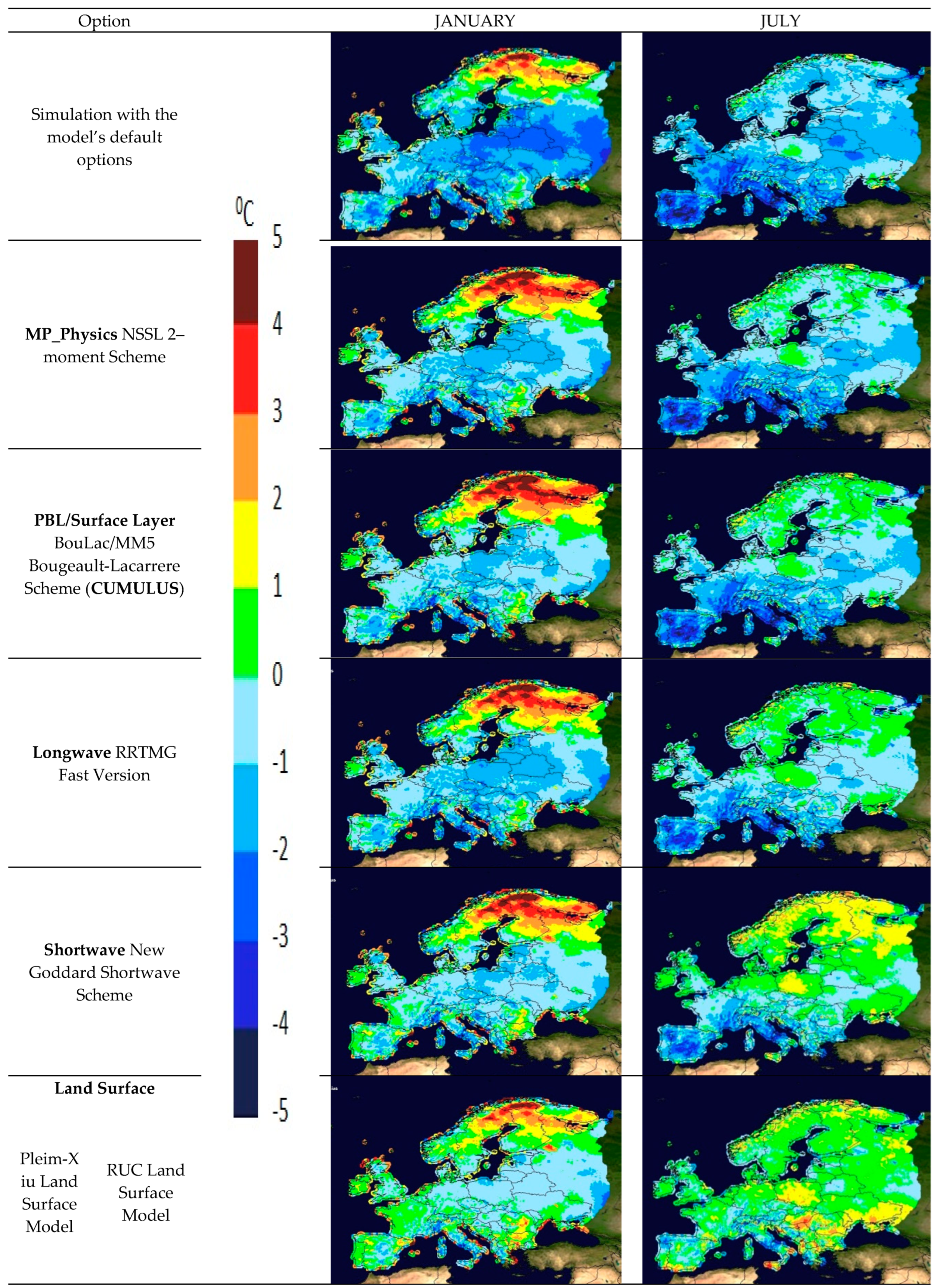
The approach followed here greatly increases the model’s prediction ability for temperature (Figure 3). Initial January simulations show significant deviations from the observed values with underestimations in central-east Europe, northern and central Italy, Greece and the Iberian up to three degrees Celsius. Overestimations are located mostly in Scandinavia reaching five degrees Celsius. Underestimations were also presented for almost all continental Europe in the initial July simulation reaching 4–5 °C in the Iberian Peninsula, France and Italy. Looking at the final simulations, it is obvious that almost all of the model’s intense failures have disappeared. There is a convergence of the grid deviations and a general smoothing without severe failures. The confined regions for model’s underestimation in January are located in central and northern Italy as well as the far east end of Europe, while model’s overestimation is found again in Scandinavia. July prediction remains poor in a very small region of central Italy and north Spain with a relatively significant underestimation, while overestimation is found in south Hungary and in the Balkans, locally.

There is no particular model deviation trend for the precipitation during January. However, significant underestimation is noticed locally in central UK, central Italy and Greece (Figure 4) and overestimation in central and North UK, north Italy, east Scandinavia and some parts of the Balkans. During July underestimation is noticed in central and Eastern Europe, locally while overestimation is found in Italy, west Greece and eastern Spain, locally. Although the strategy we pursued had the improvement of the temperature forecast as a central axis, we can see that the forecast for average precipitation has also improved to a certain extent.

4. Conclusions

PBL Bougeault-Lacarrere Scheme [29] in cooperation with the MM5 [30] Surface Layer Scheme had the best performance in predicting January and July temperature and a moderate rank for precipitation. The Yonsei University Scheme [36] is the second best choice as far as temperature prediction is concerned and winter precipitation too. If our strategy had precipitation prediction as its main axis, then the MRF/MM5 [48]/[30] combination (option 99) would be the choice we would have made.

The default Kain-Fritsch Scheme [31] gave the best results as the Cumulus parameterization scheme similar to the OSAS Old Simplified Arakawa-Schubert [32] ranking but the first was our shceme of choice as it performed better for January precipitation.

RRTMG Longwave fast version Scheme [33] scored the highest for temperature prediction and moderately for precipitation. The non-fast version of the RRTMG scheme would be our choice if our steps were precipitation driven. For shortwave radiation scheme we chose the New Goddard [35] which had a similar performance with the CAM Scheme [56]. The spatial distribution improvement of the New Goddard scheme was far better for July temperature prediction establishing it as our choice. The GFDL Shortwave Scheme [58] had the highest rank in predicting precipitation for both January and July.

Our final simulation group assessed the effect of the Land Surface model Pleim-Xiu Land Surface Model [64] performed best in predicting January temperature but poorly for July where the RUC Land Surface Model [62] produced the best results. As far as precipitation is concerned Unified Noah Land Surface Model [61] and the 5-layer Thermal Diffusion [60] performed best for January and July precipitation, respectively. To set up the model for a multiseasonal downscaling study one should choose the best performing Land Surface model for each season.

References

- Skamarock, W.C.; Klemp, J.B.; Dudhia, J.; Gill, D.O.; Barker, M.; Duda, K.G.; Huang, Y.; Wang, W.; Powers, J.G. A Description of the Advanced Research WRF, Version 3; National Center For Atmospheric Research Boulder Co Mesoscale and Microscale Meteorology Div: Boulder, CO, USA, 2008; pp. 1–113. [Google Scholar]
- Mooney, P.A.; Mulligan, F.J.; Fealy, R. Evaluation of the Sensitivity of the Weather Research and Forecasting Model to Parameterization Schemes for Regional Climates of Europe over the Period 1990–95. J. Clim. 2013, 26, 1002–1017. [Google Scholar] [CrossRef]
- Borge, R.; Alexandrov, V.; José del Vas, J.; Lumbreras, J.; Rodríguez, E. A comprehensive sensitivity analysis of the WRF model for air quality applications over the Iberian Peninsula. Atmos. Environ. 2008, 42, 8560–8574. [Google Scholar] [CrossRef]
- Bukovsky, M.S.; Karoly, D.J. Precipitation Simulations Using WRF as a Nested Regional Climate Model. J. Appl. Meteorol. Climatol. 2009, 48, 2152–2159. [Google Scholar] [CrossRef]
- Jin, J.; Miller, N.L.; Schlegel, N. Sensitivity Study of Four Land Surface Schemes in the WRF Model. Adv. Meteorol. 2010, 2010, 11. [Google Scholar] [CrossRef]
- Flaounas, E.; Bastin, S.; Janicot, S. Regional climate modelling of the 2006 West African monsoon: Sensitivity to convection and planetary boundary layer parameterisation using WRF. Clim. Dyn. 2011, 36, 1083–1105. [Google Scholar] [CrossRef]
- Haylock, M.R.; Hofstra, N.; Klein Tank, A.M.G.; Klok, E.J.; Jones, P.D.; New, M. A European daily high-resolution gridded data set of surface temperature and precipitation for 1950–2006. J. Geophys. Res. Atmos. 2008, 113. [Google Scholar] [CrossRef]
- Van den Besselaar, E.J.M.; Haylock, M.R.; van der Schrier, G.; Klein Tank, A.M.G. A European daily high-resolution observational gridded data set of sea level pressure. J. Geophys. Res. Atmos. 2011, 116. [Google Scholar] [CrossRef]
- Dudhia, J. “Overview of WRF Physics”. NCAR. Available online: http://www2.mmm.ucar.edu/wrf/users/tutorial/201601/physics.pdf (accessed on 12 June 2017).
- Hwang, C.L.; Yoon, K. Multiple Attribute Decision Making: Methods and Applications: A State-of-the-Art Survey; Springer: New York, NY, USA, 1981. [Google Scholar]
- Yoon, K. A Reconciliation Among Discrete Compromise Solutions. J. Oper. Res. Soc. 1987, 38, 277–286. [Google Scholar] [CrossRef]
- Hwang, C.-L.; Lai, Y.-J.; Liu, T.-Y. A new approach for multiple objective decision making. Comput. Oper. Res. 1993, 20, 889–899. [Google Scholar] [CrossRef]
- Shannon, C.E. A mathematical theory of communication. Bell Syst. Tech. J. 1948, 27, 379–423. [Google Scholar] [CrossRef]
- Mansell, E.R.; Ziegler, C.L.; Bruning, E.C. Simulated Electrification of a Small Thunderstorm with Two-Moment Bulk Microphysics. J. Atmos. Sci. 2010, 67, 171–194. [Google Scholar] [CrossRef]
- Kessler, E. On the continuity and distribution of water substance in atmospheric circulations. Atmos. Res. 1995, 38, 109–145. [Google Scholar] [CrossRef]
- Lin, Y.-L.; Farley, R.D.; Orville, H.D. Bulk Parameterization of the Snow Field in a Cloud Model. J. Clim. Appl. Meteorol. 1983, 22, 1065–1092. [Google Scholar] [CrossRef]
- Hong, S.-Y.; Dudhia, J.; Chen, S.-H. A Revised Approach to Ice Microphysical Processes for the Bulk Parameterization of Clouds and Precipitation. Mon. Weather Rev. 2004, 132, 103–120. [Google Scholar] [CrossRef]
- Hong, S.-Y.; Lim, J.-O. The {WRF} Single-Moment 6-Class Microphysics Scheme {(WSM6)}. J. Korean Meteor. Soc. 2006, 42, 129–151. [Google Scholar]
- Tao, W.-K.; Simpson, J.; McCumber, M. An Ice-Water Saturation Adjustment. Mon. Weather Rev. 1989, 117, 231–235. [Google Scholar] [CrossRef]
- Thompson, G.; Field, P.R.; Rasmussen, R.M.; Hall, W.D. Explicit Forecasts of Winter Precipitation Using an Improved Bulk Microphysics Scheme. Part II: Implementation of a New Snow Parameterization. Mon. Weather Rev. 2008, 136, 5095–5115. [Google Scholar] [CrossRef]
- Milbrandt, J.A.; Yau, M.K. A Multimoment Bulk Microphysics Parameterization. Part I: Analysis of the Role of the Spectral Shape Parameter. J. Atmos. Sci. 2005, 62, 3051–3064. [Google Scholar] [CrossRef]
- Milbrandt, J.A.; Yau, M.K. A Multimoment Bulk Microphysics Parameterization. Part II: A Proposed Three-Moment Closure and Scheme Description. J. Atmos. Sci. 2005, 62, 3065–3081. [Google Scholar] [CrossRef]
- Morrison, H.; Thompson, G.; Tatarskii, V. Impact of Cloud Microphysics on the Development of Trailing Stratiform Precipitation in a Simulated Squall Line: Comparison of One- and Two-Moment Schemes. Mon. Weather Rev. 2009, 137, 991–1007. [Google Scholar] [CrossRef]
- Eaton, B. “User’s Guide to the Community Atmosphere Model CAM-5.1.”. NCAR. Available online: http://www.cesm.ucar.edu/models/cesm1.0/cam (accessed on 22 May 2017).
- Lin, Y.; Colle, B.A. A New Bulk Microphysical Scheme That Includes Riming Intensity and Temperature-Dependent Ice Characteristics. Mon. Weather Rev. 2011, 139, 1013–1035. [Google Scholar] [CrossRef]
- Lim, K.-S.S.; Hong, S.-Y. Development of an Effective Double-Moment Cloud Microphysics Scheme with Prognostic Cloud Condensation Nuclei (CCN) for Weather and Climate Models. Mon. Weather Rev. 2010, 138, 1587–1612. [Google Scholar] [CrossRef]
- Gilmore, M.S.; Straka, J.M.; Rasmussen, E.N. Precipitation Uncertainty Due to Variations in Precipitation Particle Parameters within a Simple Microphysics Scheme. Mon. Weather Rev. 2004, 132, 2610–2627. [Google Scholar] [CrossRef]
- Thompson, G.; Eidhammer, T. A Study of Aerosol Impacts on Clouds and Precipitation Development in a Large Winter Cyclone. J. Atmos. Sci. 2014, 71, 3636–3658. [Google Scholar] [CrossRef]
- Bougeault, P.; Lacarrere, P. Parameterization of Orography-Induced Turbulence in a Mesobeta--Scale Model. Mon. Weather Rev. 1989, 117, 1872–1890. [Google Scholar] [CrossRef]
- Beljaars, A.C.M. The parametrization of surface fluxes in large-scale models under free convection. Q. J. R. Meteorol. Soc. 1995, 121, 255–270. [Google Scholar] [CrossRef]
- Kain, J.S. The Kain–Fritsch Convective Parameterization: An Update. J. Appl. Meteorol. 2004, 43, 170–181. [Google Scholar] [CrossRef]
- Pan, H.L. Implementing a Mass Flux Convective Parameterization Package for the NMC Medium Range Forecast Model; NMC Office Note: London, Uk, 1995; Volume 40. [Google Scholar]
- Iacono, M.J.; Delamere, J.S.; Mlawer, E.J.; Shephard, M.W.; Clough, S.A.; Collins, W.D. Radiative forcing by long-lived greenhouse gases: Calculations with the AER radiative transfer models. J. Geophys. Res. Atmos. 2008, 113, D13103. [Google Scholar] [CrossRef]
- Räisänen, P.; Barker, H.W.; Cole, J.N.S. The Monte Carlo Independent Column Approximation’s Conditional Random Noise: Impact on Simulated Climate. J. Clim. 2005, 18, 4715–4730. [Google Scholar] [CrossRef]
- Chou, M.D.; Suarez, M.J. A Solar Radiation Parameterization for Atmospheric Studies; NASA Tech. Memo 104606; NASA: Boulder, CO, USA, 1999; Volume 40.
- Hong, S.-Y.; Noh, Y.; Dudhia, J. A New Vertical Diffusion Package with an Explicit Treatment of Entrainment Processes. Mon. Weather Rev. 2006, 134, 2318–2341. [Google Scholar] [CrossRef]
- Janjić, Z.I. The Step-Mountain Eta Coordinate Model: Further Developments of the Convection, Viscous Sublayer, and Turbulence Closure Schemes. Mon. Weather Rev. 1994, 122, 927–945. [Google Scholar] [CrossRef]
- Janjic, Z.I. The surface layer in the NCEP Eta Model. In Proceedings of the Eleventh Conference on Numerical Weather Prediction, Norfolk, VA, USA, 19–23 August 1996; pp. 354–355. [Google Scholar]
- Sukoriansky, S.; Galperin, B.; Perov, V. Application of a new spectral model of stratified turbulence to the atmospheric boundary layer over sea ice. Bound. Layer Meteorol. 2005, 117, 231–257. [Google Scholar] [CrossRef]
- Nakanishi, M.; Niino, H. An improved Mellor–Yamada level 3 model: Its numerical stability and application to a regional prediction of advecting fog. Bound. Layer Meteorol. 2006, 119, 397–407. [Google Scholar] [CrossRef]
- Nakanishi, M.; Niino, H. Development of an improved turbulence closure model for the atmospheric boundary layer. J. Meteorol. Soc. Jpn. 2009, 87, 895–912. [Google Scholar] [CrossRef]
- Pleim, J.E. A Combined Local and Nonlocal Closure Model for the Atmospheric Boundary Layer. Part I: Model Description and Testing. J. Appl. Meteorol. Climatol. 2007, 46, 1383–1395. [Google Scholar] [CrossRef]
- Pleim, J.E. A simple, efficient solution of flux-profile relationships in the atmospheric surface layer. J. Appl. Meteorol. Clim. 2006, 45, 341–347. [Google Scholar] [CrossRef]
- Bretherton, C.S.; Park, S. A New Moist Turbulence Parameterization in the Community Atmosphere Model. J. Clim. 2009, 22, 3422–3448. [Google Scholar] [CrossRef]
- Angevine, W.M.; Jiang, H.; Mauritsen, T. Performance of an Eddy Diffusivity–Mass Flux Scheme for Shallow Cumulus Boundary Layers. Mon. Weather Rev. 2010, 138, 2895–2912. [Google Scholar] [CrossRef]
- Shin, H.H.; Hong, S.-Y. Representation of the Subgrid-Scale Turbulent Transport in Convective Boundary Layers at Gray-Zone Resolutions. Mon. Weather Rev. 2015, 143, 250–271. [Google Scholar] [CrossRef]
- Grenier, H.; Bretherton, C.S. A Moist PBL Parameterization for Large-Scale Models and Its Application to Subtropical Cloud-Topped Marine Boundary Layers. Mon. Weather Rev. 2001, 129, 357–377. [Google Scholar] [CrossRef]
- Hong, S.-Y.; Pan, H.-L. Nonlocal Boundary Layer Vertical Diffusion in a Medium-Range Forecast Model. Mon. Weather Rev. 1996, 124, 2322–2339. [Google Scholar] [CrossRef]
- Grell, G.A.; Freitas, S.R. A scale and aerosol aware stochastic convective parameterization for weather and air quality modeling. Atmos. Chem. Phys. 2014, 14, 5233–5250. [Google Scholar] [CrossRef]
- Grell, G.A.; Dévényi, D. A generalized approach to parameterizing convection combining ensemble and data assimilation techniques. Geophys. Res. Lett. 2002, 29, 38-1–38-4. [Google Scholar] [CrossRef]
- Tiedtke, M. A Comprehensive Mass Flux Scheme for Cumulus Parameterization in Large-Scale Models. Mon. Weather Rev. 1989, 117, 1779–1800. [Google Scholar] [CrossRef]
- Han, J.; Pan, H.-L. Revision of Convection and Vertical Diffusion Schemes in the NCEP Global Forecast System. Weather Forecast. 2011, 26, 520–533. [Google Scholar] [CrossRef]
- Zhang, C.; Wang, Y.; Hamilton, K. Improved Representation of Boundary Layer Clouds over the Southeast Pacific in ARW-WRF Using a Modified Tiedtke Cumulus Parameterization Scheme. Mon. Weather Rev. 2011, 139, 3489–3513. [Google Scholar] [CrossRef]
- Kain, J.S.; Fritsch, J.M. A One-Dimensional Entraining/Detraining Plume Model and Its Application in Convective Parameterization. J. Atmos. Sci. 1990, 47, 2784–2802. [Google Scholar] [CrossRef]
- Mlawer, E.J.; Taubman, S.J.; Brown, P.D.; Iacono, M.J.; Clough, S.A. Radiative transfer for inhomogeneous atmospheres: RRTM, a validated correlated-k model for the longwave. J. Geophys. Res. Atmos. 1997, 102, 16663–16682. [Google Scholar] [CrossRef]
- Collins, W.D.; Rasch, P.J.; Boville, B.A.; Hack, J.J.; McCaa, J.R.; Williamson, D.L.; Kiehl, J.T.; Briegleb, B.; Bitz, C.; Lin, S.-J.; et al. Description of the NCAR Community Atmosphere Model (CAM 3.0); NCAR Technical Note: Boulder, CO, USA, 2004. [Google Scholar]
- Fu, Q.; Liou, K.N. On the Correlated k-Distribution Method for Radiative Transfer in Nonhomogeneous Atmospheres. J. Atmos. Sci. 1992, 49, 2139–2156. [Google Scholar] [CrossRef]
- Fels, S.B.; Schwarzkopf, M.D. An efficient, accurate algorithm for calculating CO2 15 μm band cooling rates. J. Geophys. Res. Oceans 1981, 86, 1205–1232. [Google Scholar] [CrossRef]
- Dudhia, J. Numerical Study of Convection Observed during the Winter Monsoon Experiment Using a Mesoscale Two-Dimensional Model. J. Atmos. Sci. 1989, 46, 3077–3107. [Google Scholar] [CrossRef]
- Dudhia, J. A multi-layer soil temperature model for MM5. In Proceedings of the Preprints, the Sixth PSU/NCAR Mesoscale Model Users’ Workshop, Boulder, CO, USA, 22–24 July 1996. [Google Scholar]
- Tewari, M.; Chen, F.; Wang, W.; Dudhia, J.; LeMone, M.A.; Mitchell, K.; Ek, M.; Gayno, G.; Wegiel, J.; Cuenca, R.H. Implementation and verification of the unified NOAH land surface model in the WRF model. In Proceedings of the 20th Conference on Weather Analysis and Forecasting/16th Conference on Numerical Weather Prediction, Boulder, CO, USA, 10–15 January 2004; pp. 11–15. [Google Scholar]
- Benjamin, S.G.; Grell, G.A.; Brown, J.M.; Smirnova, T.G.; Bleck, R. Mesoscale weather prediction with the RUC hybrid isentropic-terrain-following coordinate model. Mon. Weather Rev. 2004, 132, 473–494. [Google Scholar] [CrossRef]
- Niu, G.-Y.; Yang, Z.-L.; Mitchell, K.E.; Chen, F.; Ek, M.B.; Barlage, M.; Kumar, A.; Manning, K.; Niyogi, D.; Rosero, E.; et al. The community Noah land surface model with multiparameterization options (Noah-MP): 1. Model description and evaluation with local-scale measurements. J. Geophys. Res. Atmos. 2011, 116, D12109. [Google Scholar] [CrossRef]
- Pleim, J.E.; Xiu, A. Development and Testing of a Surface Flux and Planetary Boundary Layer Model for Application in Mesoscale Models. J. Appl. Meteorol. 1995, 34, 16–32. [Google Scholar] [CrossRef]
Figure 1.
WRF multinesting domain configuration approach.
Figure 2.
Interactions between WRF parameterization schemes.
Figure 3.
Temperature Mean Bias spatial distribution after each simulation step.
Figure 4.
Precipitation Mean Bias spatial distribution after each simulation step.