The Dependence of Water Consumption on the Pressure Conditions and Sensitivity Analysis of the Input Parameters †

Faculty of Civil Engineering, Institute of Municipal Water Management, Brno University of Technology, 602 00 Brno, Czech Republic
*
Author to whom correspondence should be addressed.
†
Presented at the 3rd EWaS International Conference on “Insights on the Water-Energy-Food Nexus”, Lefkada Island, Greece, 27–30 June 2018.
Proceedings 2018, 2(11), 592; https://doi.org/10.3390/proceedings2110592
Published: 2 August 2018
(This article belongs to the Proceedings of EWaS3 2018)
Abstract
:The paper presents results and sensitivity analysis of the results of a real detailed study focused on changes in water consumption and its unevenness with changing pressure conditions in a particular observed office building. The dependence of water consumption on pressure is expressed using the FAVAD equation using the N3 coefficient. Parameters for sensitivity analysis are number of workers in the building, pulse value from water meter and length of time step for expressing unevenness of water consumption during the day.
1. Introduction
At present, the effective implementation of water supply systems is a major task. This basically means that an optimization of selected optimization criteria was carried out according to chosen preferences, based on changes in operating parameters affecting the selected criteria. Now, the water losses, respectively its reducing, is mostly frequently used as an optimization criterion, and the energy recuperation as well [1,2]. Both of these criteria have in most cases the opposite desired extreme, and in particular, it is necessary to reduce the pressure in the water system for reducing water losses. However, the pressure drop will also reduce the part of water consumption. When optimizing pressure conditions in water systems, water consumption should also be taken into account as a criterion. In contrast to the two above-mentioned criteria, water consumption is also burdened by a higher stochasticity and by various factors as well. Factors influencing the consumption include a group of operating factors, with the pressure in the water system being most influential among them, for example according to [1,2,3,4,5,6], the climatological factors [6,7,8,9] and also, for example, the water price [2,10,11].
For water consumption is valid that for each type of a user, the dependency on factors influencing consumption is always different [12]. Water consumption is divided into “inside the house” and “outside the house” for the prediction of water consumption with pressure variation [13]. Both parts of the consumption then have different coefficients expressing the dependency on pressure. Subsequently, the average coefficient expressing the dependency of pressure for the entire building respectively for one consumer is calculated. Subsequently, this cumulative coefficient for one user is implemented into the FAVAD (Fixed and Variable Discharge) equation according to [14], respectively into its simplified form according to [13]. Nowadays, there are not too many N3 set coefficients within the meaning of [13] based on real studies. Value of this coefficient explains degree of dependency of water consumption on pressure. However, for example the value of the “inside the house” consumption coefficient was set at 0.2 for the Johannesburg students ‘campus in [15]. According to [16], the dependence of consumption on pressure for pressure flushers in Great Britain was also demonstrated and the value of the coefficient was set at 0.07 and 0.025. The course of water consumption over time under various pressure conditions was given attention in the study [17], where the dependence of the water consumption during the day on the pressure conditions was determined.
This article builds on the detailed real-life study and the established results that have been presented in [8,17]. This study was focused on monitoring the influence of pressure on water consumption and its course over time for an office building. This paper presents a sensitivity analysis of the results presented in [8,17], where the influence of the input parameters on the results obtained was monitored. The monitored input parameters are in this case the number of people in the building during the working time, the water meter pulse value and the time step length in the characterization of the water consumption using demand coefficients.
2. Methodology
A detailed description of the procedure of the study data evaluation aimed at monitoring the influence of pressure on water consumption and its course over time is described in [8,17]. This article only presents the necessary mathematical approach for determining the N3 coefficient and the demand coefficients.
To determine the N3 coefficient, first it was necessary to take into account that working hours are not the same every working day. This means that the consumption per working day was related to the selected time unit, in this case it was 1 h. In [8] the influence of the number of workers in the building during working hours was also included. For further comparison, the format was considered litre-1.person-1.hour-1. According to the relation:
where Ci is the standard water consumption for the ith day (for working hours of the day), Vi is the volume of water consumed during the ith working day, pi is the number of people on the shift of the ith day, and hi is the number of working hours on the ith day. For the purposes of performing the sensitivity analysis in this article, the value of the N3 coefficient was calculated without including the number of shift workers, with the relationship (1) being then adjusted as follows:
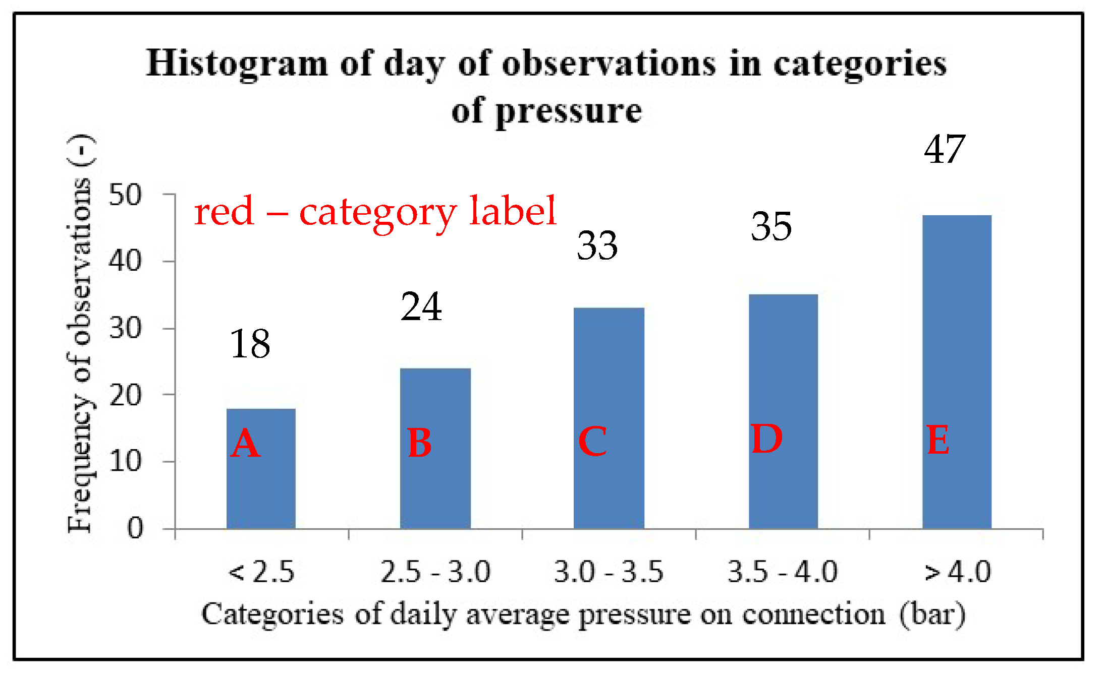
For other needs for determining the N3 coefficient, the individual working days are classified into pressure categories according to the average daily pressure (during the working hours of the given day). The categorization has been done with respect to the balance of the number of values in each class, but also with respect to the size of the intervals of the individual categories. The criterion was also the absolute number of values in each category. The category division is shown in Figure 1. The value of the N3 coefficient was determined in the meaning of [13]. This coefficient was set on the basis of the average values of water consumption and pressure for each category according to the following relations:
where C1k is the actual water consumption for the kth category, C1k is the calculated water consumption for the kth category, wk is the weight of the kth category determined by [8] and m is the number of pressure categories. It follows from this equation that the weighted square deviation of the calculated water consumption values from the actual measured water consumption for the given pressure category has been minimized. The consumption was calculated according to the following formula with accordance to [13]:
where C0 is the water consumption for the highest pressure category, P1k is the mean pressure in the kth pressure category, P0 is the mean pressure in the highest pressure category, and N3 is the coefficient expressing the effect of the change in pressure conditions on the water consumption.
In the second part of the sensitivity analysis, attention is paid to the course of water consumption during the day. To determine the coefficients of the unevenness (demand coefficients) and the maximum coefficient for the selected time step, the following procedure is used:
Flow in the time step j, in day i is determined as average flow in day i multiplied by coefficient in the time step j during day i.
where Qij represents flow, QMEANi is mean flow, cij is coefficient of water demand variation.
Coefficient of variation after modification is determined as follows:
Mean coefficient for each time step in pressure category k is determined as the sum of all coefficient values in time step j, in the pressure category k.
where cMEANik is mean coefficient, k is pressure category, mk is the total number of days in category k.
where cMAXk [-] is the maximal coefficient in k category.
where εk [-] represents square deviation of coefficients from optimal value in each time step (as optimal value is considered 1. It corresponds to constant consumption during day).
3. Case Study
The aim of this study was to monitor the change in water consumption with the dependencies of the change in pressure in the internal water supply of the building. The pressure was gradually controlled by a special pressure regulating valve on the water service connection, which is connected to the public water supply system. Experiment was conducted on an office building, which is a relatively common type of building in a consumption area up to the size of a regional city. This building has three above-ground floors and the maximal number of workers is 35. The workers are practically evenly divided into each of the above-ground floors, in which identical equipment is provided. To determine the anomalies in the measured statistical data set, the number of people in the building was monitored on working days. The evaluation of dependencies took place only during the working days. The duration of the measurement campaign in the case study was one calendar year. The survey found out that in the meaning of [13] all measured water was consumed “inside the house”.
Throughout the experiment, a continuous pressure and water flow measurement on the output of the control valve was conducted in the pipeline of the internal water supply. The pressure was measured with an integrated pressure sensor with a range of 0.0–1.0 MPa with a measurement accuracy of 0.25% of the range. Measured pressure values were stored with a time period of 15 s. The volume of water per time unit was measured with a precision water meter of the “C” type with a pulse generator. The pulse value was set to 1 L. Measuring of the volume with this pulse size allowed a sensitivity analysis to indicate the influence of the pulse size on the value of the N3 coefficient. The simulation of the pulse size was performed in the way that at each time the water meter was recorded, this state was rounded to the nearest lower multiple of the selected pulse size.
For this case study, the intervals of the pressure conditions categories and the number of values in individual categories are shown in Figure 1. The value of the pressure of one day was determined as the arithmetic mean of the considered working hours of the given day.
As can already be seen from Figure 1, the total number of observations is 157. Due to the range of maximum and minimum pressures (1.96–4.19 bar), a division into 5 categories was chosen. The boundaries of these categories and their indication are shown in Figure 1.
There are three working time shifts in the studied building: 7:00 to 17:00 on Mondays and Wednesdays, 7:00 to 15:00 on Tuesdays and Thursdays and 7:00 to 13:00 on Fridays. A common working time for all days was selected for sensitivity analysis of the established demand coefficients (from 7:00–13:00).
The following values of water consumption were characteristic for the studied building.
Based on the values given in Table 1, pulse values were selected. As it can be seen, the average hourly consumption (“AHC”) is approximately 90 L h−1. The pulse value was chosen as a percentage of this value, but also respected the technical practice and commonly used pulse values. The relative pulse value considering AHC was chosen as 2.5, 5, 10, 20, 50 and 100%, which in absolute values corresponded to the pulse size of 2, 5, 10, 20, 50 and 100 L.
4. Results
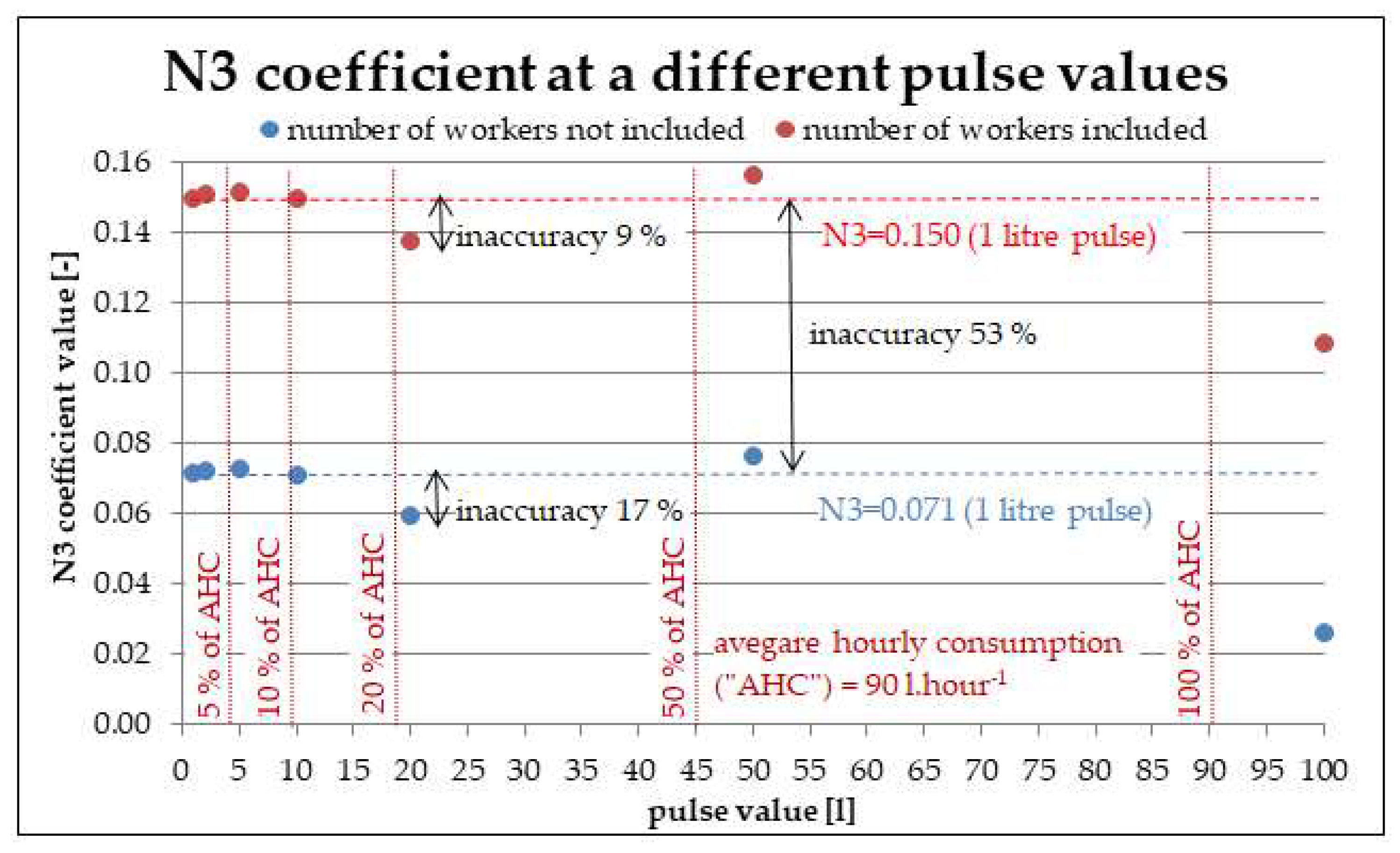
The N3 coefficient for changing input parameters was determined on the basis of Equations (1)–(4). Achieved results of the sensitivity analysis of N3 value are well evident from Table 2 and Figure 2.
As it can be seen in Figure 2 and Table 2, the monitoring of a number of workers during the day has a big impact on the N3 coefficient values. Inaccuracies when determining the value of the N3 coefficient without monitoring the number of people in the building and with the monitoring amount at 53%, even when considering the smallest pulse of 1 L (real measurement). In case the number of workers was observed, it was found out that up to 10% of AHC the high accuracy of the N3 value is achieved.
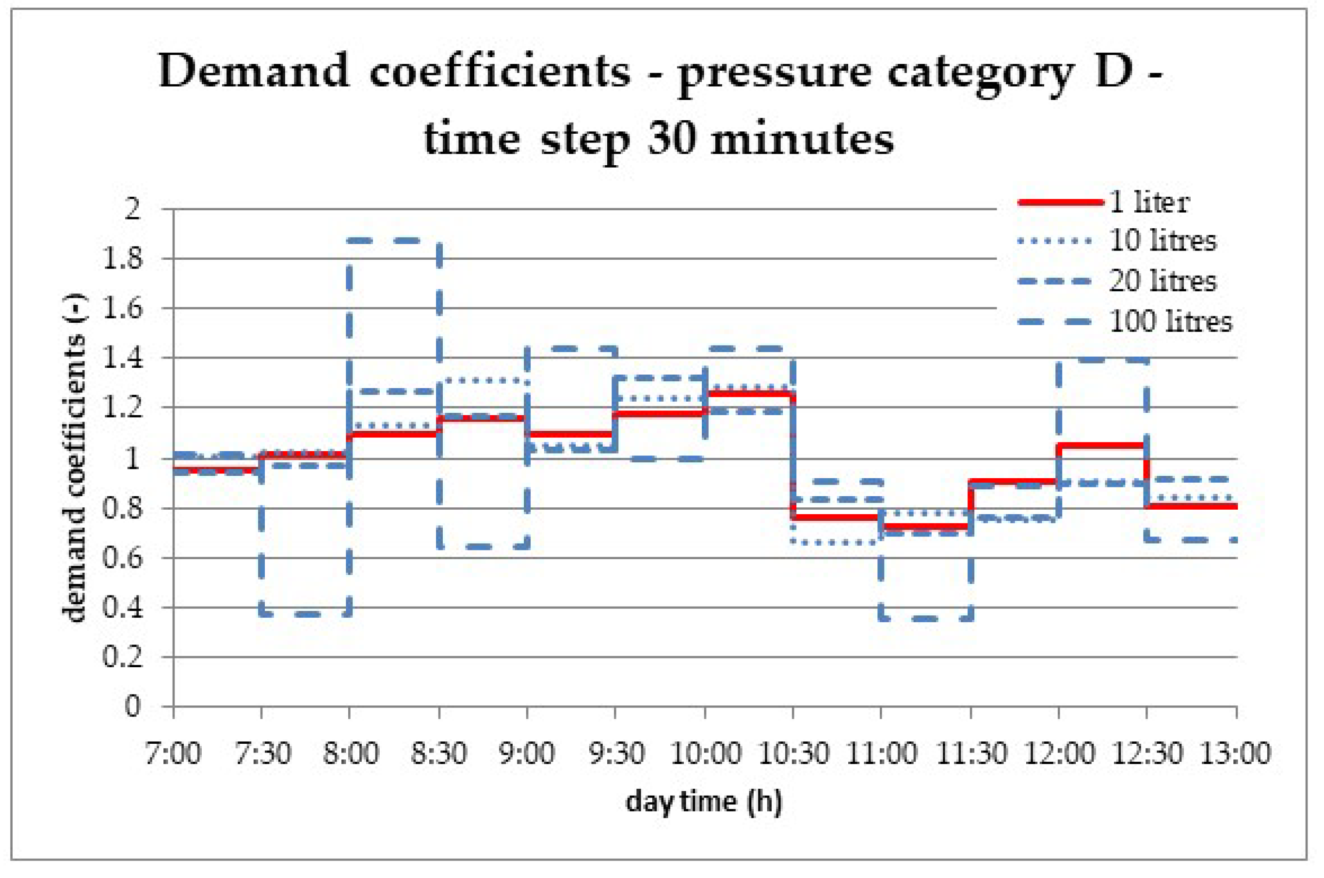
The unevenness of water consumption, respectively its time course was analyzed for all the pressure categories. In these cases, samples (5)–(7) were used to calculate the coefficients. In this article only the most interesting results for the selected pressure categories and the time step are chosen. It is graphically well-known in Figure 3 (30 min time step) that increasing the pulse value results in greater variance of the coefficient values than the most accurately set values (pulse value of 1 L). Increased variance of coefficient values begins when the pulse value exceeds 5% of AHC.
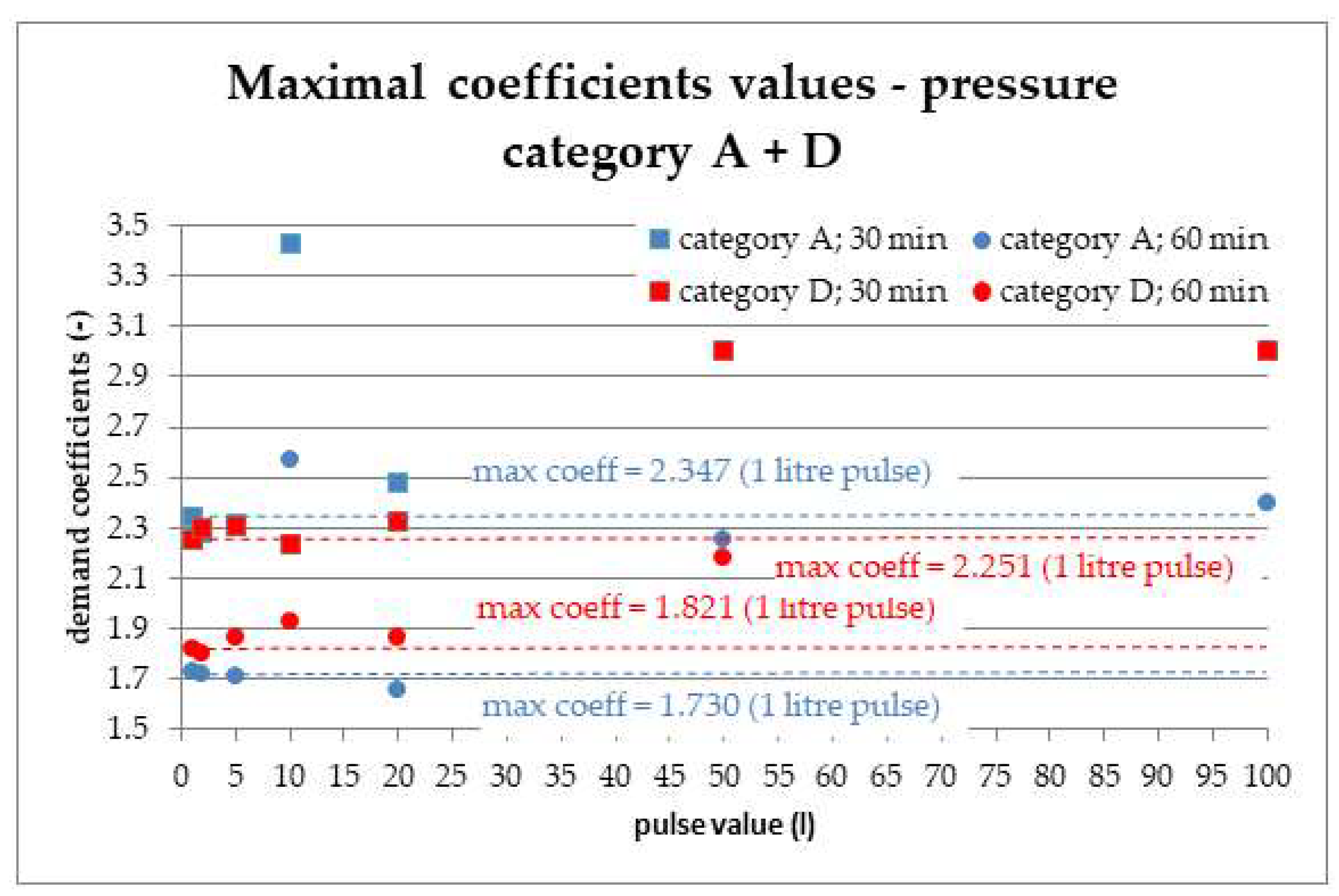
Similar trends and results are achieved for other categories and time step lengths. The results of the sensitivity analysis for the maximum coefficients for the given time step for each pressure category are also interesting. Figure 4 shows a trend of the increasing maximum value of the demand coefficients with the increase in pulse size. Relatively satisfactory accuracy for all categories is achieved up to a pulse size of 5% AHC. The values of the maximum coefficients and the accuracy in determining the maximum coefficient value (compared to the pulse value of 1 L) for a 30 min time step for all categories are apparent from Table 3 respectively Table 4.
5. Discussion
At present, there is still not enough realistic studies carried out on the impact of pressure ratios on water consumption, as opposed to, for example, the loss of water that has been and is being paid much attention to. In future, more studies will be needed, such as [8]. The problem of conducting realistic studies is the need to change the pressure conditions, which can cause customer complaints at the lower and upper limits of the allowed pressure range in the distribution network even if the legal requirements are met. As the relationship pressure: consumption will be necessary to describe in the future, this article provides some guidance on what to pay attention to during similar studies, and what impact the inaccuracy of the input data may have on the results achieved.
There are many possibilities to carry out more real measurements in the near future. This option is based on the use of SMART metering, which will allow to collect water consumption information at short time intervals for different types of customers. From these data, it would be possible in the future to be able to compile complex dependences of the unevenness of the distribution for the whole distribution network, not just for individual types of customers.
6. Conclusions
This paper presents the results of the sensitivity analysis based on the studies [8], and it was found out that when determining the value of the N3 coefficient for an office building, the most important input parameter was the number of workers in the building during individual working days. The most accurately determined value was 0.150 (with a pulse value of 1 L and with monitoring the number of workers), while retaining a pulse value of 1 L and not including the number of workers, the value of the N3 coefficient was only 0.071, that makes the inaccuracy of 53%. This high inaccuracy in determining the N3 coefficient was not found out even in the case of a pulse size of 100 L (approximately 110% of the average hourly consumption) when the inaccuracy of the N3 value was 27%. The inaccuracy of the N3 determination increased with the increasing pulse value, but the N3 set values up to 10% of the AHC and 10 L, respectively, were considered to be accurate enough, with the inaccuracy of <2% in both cases.
A sensitivity analysis of demand coefficients describing the course of water consumption over time has shown that the inaccuracy when determining the coefficients in the chosen time steps is acceptable up to a pulse size of 5% of AHC. The highest inaccuracy found over a 30 min time step is only 7% up to a pulse size of 5% of AHC, which can still be considered satisfactory.
Based on the results presented here, it is possible to provide for similar future studies such as [8]. To determine the N3 coefficient, for example, for an office building, it is absolutely essential to monitor the number of shift workers, which guarantees that even if the pulse value is badly selected, the result will not be burdened with such a large error. However, for the determination of the N3 value, the pulse value should not exceed 10% of the AHC. It is very unsuitable to use pulse values of >20% of AHC. To monitor the water consumption process over time and determine the maximum coefficients in the selected time steps, it is advisable that the pulse size does not exceed the 5% pulse value of the AHC.
Finally, it should be noted that studies [8] were carried out for the office building type, so it is not appropriate to apply the above-mentioned values and conclusions globally to each type of a consumer. However, there is a presumption that the observed dependencies will be similar to other types of consumers and therefore the above mentioned recommendations can be applied to other types of consumers with a certain tolerance dose.
Author Contributions
T.S. and L.T. designed the methodology and the measuring experiment. T.S. and J.R. assembled the measuring device, analyzed the data and wrote the paper.
Funding
This research work is funded by the Brno University of Technology.
Acknowledgments
This research work is funded by the Brno University of Technology in the frame of the research projects titled FAST-J-18-5339 Experimental determination of dependency of withdrawn water from the tap on pressure conditions and FAST/FSI-J-18-4569 Visualization of hydraulic analysis results in virtual reality.
Conflicts of Interest
The founding sponsors had no role in the design of the study; in the collection, analyses, or interpretation of data; in the writing of the manuscript, and in the decision to publish the results.
References
- Patelis, M.; Kanakoudis, V.; Gonelas, K. Pressure Management and Energy Recovery Capabilities Using PATs. Procedia Eng. 2016, 162, 503–510. [Google Scholar] [CrossRef]
- Kanakoudis, V.; Gonelas, K. The joint effect of water price changes and pressure management, at the economic annual real losses level, on the system input volume of a water distribution system. Water Sci. Technol. Water Supply 2015, 15, 1069–1078. [Google Scholar] [CrossRef]
- Bamezai, A.; Lessick, D. Water Conservation through System Pressure Optimization in Irvine Ranch Water District; Western Policy Research: Irvine, CA, USA, 2003. [Google Scholar]
- Wagner, J.M.; Shamir, U.; Marks, D.H. Water distribution reliability: simulation methods. Water Resour. Plan. Manag. 1988, 114, 276–294. [Google Scholar] [CrossRef]
- Cullen, R. Pressure vs. Consumption Relationships in Domestic Irrigation Systems. Bachelor’s Thesis, University of Queensland, Saint Lucia, QLD, Australia, 2004. [Google Scholar]
- Xenochristou, M.; Kapelan, Z.; Hutton, C.; Hofman, J. Identifying Relationships between Weather Variables and Domestic Water Consumption Using Smart Metering. In Proceedings of the CCWI—Computing and Control for the Water Industry, Sheffield, UK, 5 September 2017. [Google Scholar]
- Praskievicz, S.; Chang, H. Identifying the Relationships between Urban Water Consumption and Weather Variables in Seoul, Korea. Phys. Geogr. 2009, 30, 324–337. [Google Scholar] [CrossRef]
- Suchacek, T.; Tuhovcak, L.; Ruckaj, J. Influence of pressure, temperature and humidity on water consumption. In Proceedings of the CCWI—Computing and Control for the Water Industry, Sheffield, UK, 8 September 2017. [Google Scholar]
- Viscor, P.; Prokop, L. Meteorological conditions and daily water requirements of the Brno Water Supply System (in Czech). In Proceedings of the Voda Zlin 2016, Zlin, Czech republic, 17 March 2016; Moravska Vodarenska: Olomouc, Czech Republic, 2016; pp. 41–46. [Google Scholar]
- Kanakoudis, V.; Gonelas, K. The Optimal Balance Point between NRW Reduction Measures, Full Water Costing and Water Pricing in Water Distribution Systems. Alternative Scenarios Forecasting the Kozani’s WDS Optimal Balance Point. Procedia Eng. 2015, 119, 1278–1287. [Google Scholar] [CrossRef]
- Kanakoudis, V.; Gonelas, K. Forecasting the Residential Water Demand, Balancing Full Water Cost Pricing and Non-revenue Water Reduction Policies. Procedia Eng. 2014, 89, 958–966. [Google Scholar] [CrossRef]
- Hussien, W.A.; Memon, F.A.; Savic, D.A. Assessing and Modelling the influence of household Characteristics on Per Capita Water Consumption. Water Res. Manag. 2016, 30, 2931–2955. [Google Scholar] [CrossRef]
- Lambert, A.O.; Fantozzi, M. Recent developments in pressure management. In Proceedings of the Water Loss, Sao Paolo, Brazil, 6–9 June 2010. [Google Scholar]
- May, J. Pressure dependent leakage. World Water Environ. Eng. 1994, 17, 10. [Google Scholar]
- Bartlett, L.B. Eng Final Year Project Report. In Pressure Dependent Demands in Student Town Phase 3; Department of Civil and Urban Engineering, Rand Afrikaans University (now University of Johannesburg): Johannesburg, South Africa, 2004. [Google Scholar]
- Thorton, J.; Lambert, A. Progress in practical prediction of pressure: leakage, pressure: Burst frequency and pressure: consumption relationships. In Proceedings of the IWA Special Conference ‘Leakage 2005’, Halifax, NS, Canada, 12–14 September 2005. [Google Scholar]
- Suchacek, T.; Tuhovcak, L.; Ruckaj, J. Sensitivity analysis of water consumption in an office building. E3S Web Conf. 2018, 30. [Google Scholar] [CrossRef]
Figure 1.
Histogram of number of pressure measurements in pressure categories.

Figure 2.
The N3 coefficient values of changing input parameters.

Figure 3.
Demand coefficients for pressure category D for 30 min time step.

Figure 4.
Maximal coefficients values for pressure categories A + D.


Table 1.
Characteristic values of water consumption during working hours.
| Water Consumption in Working Hours | Minimal Consumption | Mean Consumption | Maximal Consumption |
|---|---|---|---|
| Day (Working Hours) | (Liters) | (Liters) | (Liters) |
| Monday + Wednesday (7–17) | 608 | 892 | 1307 |
| Tuesday + Thursday (7–15) | 481 | 710 | 1252 |
| Friday (7–13) | 307 | 623 | 927 |
| All days (7–13) | 307 | 545 | 982 |
Table 2.
The N3 coefficient values depending on pulse size.
| N3 Coefficient Value | Pulse Value (Liter) | ||||||
|---|---|---|---|---|---|---|---|
| 1 | 2 | 5 | 10 | 20 | 50 | 100 | |
| number of workers not included | 0.071 | 0.072 | 0.072 | 0.071 | 0.059 | 0.076 | 0.026 |
| number of workers included | 0.150 | 0.151 | 0.151 | 0.150 | 0.137 | 0.157 | 0.109 |
Table 3.
Square deviation for a time step of 30 min.
| εk (-) | Pulse Value (Liter) | ||||||
|---|---|---|---|---|---|---|---|
| Pressure Category | 1 | 2 | 5 | 10 | 20 | 50 | 100 |
| A | 0.475 | 0.486 | 0.484 | 0.466 | 0.436 | 0.677 | 2.363 |
| B | 0.325 | 0.333 | 0.342 | 0.508 | 0.376 | 0.455 | 0.799 |
| C | 0.394 | 0.387 | 0.385 | 0.417 | 0.469 | 0.394 | 0.809 |
| D | 0.496 | 0.466 | 0.500 | 0.521 | 0.461 | 0.517 | 0.957 |
| E | 0.431 | 0.434 | 0.442 | 0.410 | 0.418 | 0.435 | 0.580 |
Table 4.
Percent inaccuracy compared to a pulse value of 1 L for a time step length of 30 min.
| Inaccuracy (%) | Pulse Value (Liter) | ||||||
|---|---|---|---|---|---|---|---|
| Pressure Category | 1 | 2 | 5 | 10 | 20 | 50 | 100 |
| A | - | 2 | 1 | 4 | 6 | 55 | 249 |
| B | - | 2 | 3 | 49 | 26 | 21 | 76 |
| C | - | 2 | 0 | 8 | 13 | 16 | 105 |
| D | - | 6 | 7 | 4 | 11 | 12 | 85 |
| E | - | 1 | 2 | 7 | 2 | 4 | 33 |
Publisher’s Note: MDPI stays neutral with regard to jurisdictional claims in published maps and institutional affiliations. |
© 2018 by the authors. Licensee MDPI, Basel, Switzerland. This article is an open access article distributed under the terms and conditions of the Creative Commons Attribution (CC BY) license (https://creativecommons.org/licenses/by/4.0/).
Share and Cite
MDPI and ACS Style
Tuhovcak, L.; Suchacek, T.; Rucka, J. The Dependence of Water Consumption on the Pressure Conditions and Sensitivity Analysis of the Input Parameters. Proceedings 2018, 2, 592. https://doi.org/10.3390/proceedings2110592
AMA Style
Tuhovcak L, Suchacek T, Rucka J. The Dependence of Water Consumption on the Pressure Conditions and Sensitivity Analysis of the Input Parameters. Proceedings. 2018; 2(11):592. https://doi.org/10.3390/proceedings2110592
Chicago/Turabian StyleTuhovcak, Ladislav, Tomas Suchacek, and Jan Rucka. 2018. "The Dependence of Water Consumption on the Pressure Conditions and Sensitivity Analysis of the Input Parameters" Proceedings 2, no. 11: 592. https://doi.org/10.3390/proceedings2110592