Low-Altitude Terrain-Following Flight Planning for Multirotors
by
 , , ,
, , ,
Carmelo Donato Melita
 ,
,
Dario Calogero Guastella
*,
Luciano Cantelli
,
Giuseppe Di Marco
,
Irene Minio
and
Giovanni Muscato

Dipartimento di Ingegneria Elettrica, Elettronica e Informatica, Università di Catania, 95125 Catania, Italy
*
Author to whom correspondence should be addressed.
Drones 2020, 4(2), 26; https://doi.org/10.3390/drones4020026
Submission received: 23 May 2020
/
Revised: 22 June 2020
/
Accepted: 23 June 2020
/
Published: 25 June 2020
Abstract
:Surveying with unmanned aerial vehicles flying close to the terrain is crucial for the collection of details that are not visible when flying at higher altitudes. This type of missions can be applied in several scenarios such as search and rescue, precision agriculture, and environmental monitoring, to name a few. We present a strategy for the generation of low-altitude trajectories for terrain following. The trajectory is generated taking into account the morphology of the area of interest, represented as a georeferenced Digital Surface Model (DSM), while ensuring a safe separation from any obstacle. The surface model of the scenario is created by using a UAV-based photogrammetry software, which processes the images acquired during a preliminary mission at high altitude. The solution was developed, tested, and verified both in simulation and in real scenarios with a multirotor equipped with low-cost sensing. The experimental results proved the validity of the generation of trajectories at altitudes lower than most of the works available in the literature. The images acquired during the low-altitude mission were processed to obtain a high-resolution reconstruction of the area as a representative application result.
1. Introduction
Data acquisition for monitoring and mapping from Unmanned Aerial Vehicles (UAVs) is a widely explored approach because of the possibility to cover wide areas and to fly over inaccessible and sometimes dangerous zones [1,2]. An aerial vehicle allows the intervention in a wide (unknown) region and/or in a scenario that is modified by a catastrophic event (such as an earthquake, a landslide, a volcanic eruption, etc.), where collecting data from the ground is neither simple nor safe [3,4,5,6].
In some cases, it is important to execute flights at very low altitudes, thus capturing details that are not visible when flying at higher altitudes. For example, in the case of an earthquake, one of the objectives of the mission can be to look for survivors by flying as close as possible to collapsed buildings [7]. In the case of a landslide or a mudslide, it could be helpful to fly following the slope of the terrain [8,9]. One of the goals of the mission can be to reconstruct an accurate map or a 3D model of the zone, with a high degree of resolution, to perform precise measurements [10,11]. Estimates of the volume of a landslide or the measurement of the quantity of lava ejected from a volcanic vent are key factors that help the experts to better understand the event’s progress. The analysis of small ground deformations allows the monitoring and, in some cases, the prediction of geological hazards [12,13]. Low-altitude flights were also explored as solutions for yield estimation and precision agriculture [14,15]. All of the above examples prove the need for having hardware and software techniques enabling a UAV to follow low-altitude trajectories that take into account the geometry of the scenario.
The solution proposed in this paper provides a survey approach to be applied for the intervention with multirotors, in order to perform highly detailed low-altitude missions following the morphology of the area of interest. To this end, several aspects are considered in the trajectory generation, ranging from the vehicle localization accuracy to the rotor downwash flow. The proposed methodology exploits a georeferenced Digital Surface Model (DSM) of the scene built from UAV-based photogrammetry. Moreover, our implementation is suited to low-cost hardware.
The remainder of this paper is structured as follows. In Section 2 an overview of the current state of the art about low-altitude flight planning is given. Our solution is briefly introduced in Section 3 and the details are given in the following sections. Section 4 introduces the reconstruction of the environment from aerial images, while Section 5 presents the processing performed on the environment model. The trajectory generation method is explained in Section 6. Section 7 is dedicated to the presentation of the experimental setup. The results of the simulations are reported and discussed in Section 8, while the results obtained in the real testing scenarios are reported and analysed in Section 9. Finally, conclusions and future developments are reported in Section 10.
2. Related Work
In the related literature, a recurring approach for the collection of detailed ground data of an unknown area is to employ UAVs equipped with cameras. Such kind of flight planning is typically referred to as terrain-following because it takes into account the specific morphology of the terrain or of the area to inspect.
A control strategy called optiPilot is presented in [16], which allows a fixed wing UAV to fly autonomously, following the terrain at an altitude of about 9 m Above Ground Level (AGL) and reacts to the presence of static obstacles by using a set of custom designed optical flow detectors. This strategy represents a first solution to the problem of flight at a medium altitude, by using a sensors-to-actuator control strategy. The output of the optical flow algorithm, which is used to detect obstacles, is mapped into the roll and pitch control signals, thereby allowing the vehicle to turn and change altitude. This is a weakness of such an approach because it needs dedicated and custom hardware, and its porting to most mass-market UAVs and autopilots could be burdensome. Moreover, this strategy, which is based on the adoption of optical flow, could be unusable in the case of uniform surfaces and/or where it is hard to find visual keypoints, such as a snow field, a landslide, or a lava field. A similar optical-flow-based solution is proposed also in [17] where the lowest altitude reached during the experiment is 25 m AGL.
In [18] the authors developed a mission planning solution with altitude constraints in an open field with terrain mounds as obstacles. The path planning algorithm adopted is based on the fast marching square method. The reported results are related to simulations only and the algorithm was tested with an altitude of 2, 5, and 10 m AGL. A robust control strategy for low-altitude flights is presented in [19]. In this work, the authors developed a second-order hexacopter dynamics model with localization and pose feedback provided by barometer, GPS and IMU. Thanks to the developed strategy, the authors were able to fly between 2 and 6 m AGL. However, they do not deal with the problem of flying following the terrain profile.
Several guidance strategies for low-altitude navigation of an unmanned helicopter are presented in [20], including a laser ranging sensor, which is mounted under the nose of the vehicle, to scan the terrain. However, this approach requires expensive sensing and control payload and is computationally intensive.
Additionally, several commercial and software solutions were proposed that allow an aerial vehicle to fly following the terrain. A terrain following flight mode was introduced in recent firmware releases of the open source ArduPilot autopilot suite (https://ardupilot.org/copter/docs/terrain-following.html last accessed on 2020/06/14). In this case, a database of the area of interest, containing the terrain height in meters above sea level, must be previously uploaded onto the autopilot storage from the Ground Control Station (GCS). During the flight, the autopilot uses the terrain data to maintain a constant altitude over the ground. However, it is recommended to fly at an altitude of 60 m AGL or more, due to the low accuracy of the terrain information available in the GCS database. Downward facing LIDAR or sonar sensors are suggested for lower altitudes.
The multirotor manufacturing company DJI proposes a Guidance System. The Guidance Core processor integrates the information coming from five on-board stereo cameras and five ultrasonic sensors to provide real-time data about the surrounding environment, such as distance from nearby obstacles and velocity. However, a suitable on-board navigation system must be able to receive and properly handle these data to implement obstacle avoidance and terrain following algorithms and DJI suggests the adoption of further proprietary hardware. Although this type of architecture is extremely simple if only DJI components are used, it is rather expensive and a great effort is required in the integration of third-party navigation systems. Moreover, the DJI system does not take into account any a priori knowledge of the environment, which may be used to optimize the mission planning of the UAV.
3. Proposed Solution
Our method was developed with the aim to perform terrain-following flying missions at lower altitudes (namely below 10 m AGL) compared to the methods described in the previous section. We are also able to assign the desired velocity for the mission execution, thus having the opportunity to slow down or speed up the flight taking also into account the vehicle’s performance. Moreover, in contrast to the strategies discussed above, our approach is also suitable to low-cost UAVs with limited on-board computing resources. In fact, the outcome of our workflow is a sequence of waypoints that can be imported from most of the commercial autopilots.
Assuming a digital surface model of the environment is available, the workflow of our method is structured as follows:
- the DSM of the environment is downsampled (if needed), dilated and smoothed;
- the desired Points of Interest are selected on the DSM;
- the 3D trajectory is computed and exported in a comma-separated values (CSV) file;
- the trajectory file is uploaded to the on-board autopilots, thus making the UAV ready to autonomously execute the mission.
During the development phase, the efficiency and the robustness of the method were verified in simulation. After that, the method was tested in two real scenarios. We performed a preliminary on-field trial in a landslide-like area within a semi-urban environment (37.536305° N, 15.069432° E). Finally, we surveyed a post-eruption volcanic area, the lava flow of the July–August 2001 Mount Etna eruption (37.667273° N, 14.999786° E).
4. Surface Model Reconstruction
A photogrammetry software for drone-based mapping is adopted for the 3D reconstruction, Pix4Dmapper (https://www.pix4d.com/product/pix4dmapper-photogrammetry-software last accessed on 2020/06/14) by Pix4D. Briefly, the reconstruction process is based on the automatic extraction and matching of visual keypoints between the acquired aerial images, which are then used to derive the pose (i.e., the attitude and the position) of the camera during the flight. After that, the 3D coordinates of the keypoints are calculated by taking into account the reconstructed camera pose. The DSM is obtained from the point cloud of the filtered and interpolated 3D points. The output is a GeoTIFF file, a raster file that encodes elevation data in the pixel values as well as the geographic data.
The flight plan for the image acquisition has to be organized to guarantee that a large number of keypoints can be matched, i.e., a sufficient overlap between the captured pictures is ensured. This is achieved by following a back-and-forth pattern at a high altitude.
The accuracy of the reconstructed model highly depends on the Ground Sampling Distance (GSD), i.e., the real-world distance on the ground between two consecutive pixels’ centers in the acquired image [21]. The flight height h above ground level is related to the parameters of the camera (sensor width, focal length, image width) and to the GSD of the single image by the following:
Pix4Dmapper needs some additional information in order to georeference the model. Specifically, the positions of the images must be known in order to locate, scale, and orientate correctly the model. This information is automatically imported from the images if a geo-tagging system is used to save the GPS coordinates in the image files. Therefore, the accuracy of the georeferenced model is closely related to the accuracy of the on-board GPS used for geo-tagging. Although Pix4Dmapper averages the positions, the inaccuracy in the coordinates may lead to large errors in the position of the model. In general, accuracy can be increased in two ways [22]:
- by using a more accurate localization system, such as a Real-Time Kinematic (RTK) Global Navigation Satellite System (GNSS) receiver;
- by introducing Ground Control Points (GCPs) in the process, which are points with known coordinates. These points must be clearly visible in the acquired pictures, because they have to be manually marked in the mapping software with the known coordinates.
Typically, Ground Control Points are chosen in the area surrounding the region of interest and their coordinates are measured by using topographic equipment, such as a so-called total station or a precise GNSS receiver. Alternatively, if the area is not accessible, the GCPs can be derived from other sources, such as existing geospatial data or Web Map Service. As will be described later, the georeferencing accuracy of the reconstructed model is one of the parameters that are taken into account in the generation of the trajectory.
In our case, we performed an autonomous survey by capturing images of the volcanic testing area with a 12 megapixel camera stabilized through a 3-axis gimbal. Besides the geo-tagging system of the images, four GCPs were used to improve the accuracy of the surface model. Their positions were measured with a Leica Viva GS10, a high-precision GNSS receiver achieving centimeter accurate positioning. The on-field measurement of the GCPs’ coordinates was preferred to the selection of GCPs available from web map services, as the latter provide data with much lower accuracy. A minimum number of 3 matches and a 7 × 7 pixel matching window size were chosen as mesh processing options in Pix4Dmapper, whereas the DSM is generated via Inverse Distance Weighting method. Figure 1 shows the outputs of Pix4Dmapper for our testing area: the orthomosaic and the DSM. The average GSD obtained with a 20 m-high survey is 1.26 cm/pixel. However, it must be underlined that this value is not derived from Equation (1). It is a value assessed by Pix4Dmapper for the final DSM by averaging the acquired images’ positions, corrected through keypoint matching, geo-tagging and GCPs coordinates. The textured 3D mesh is represented in Figure 2.
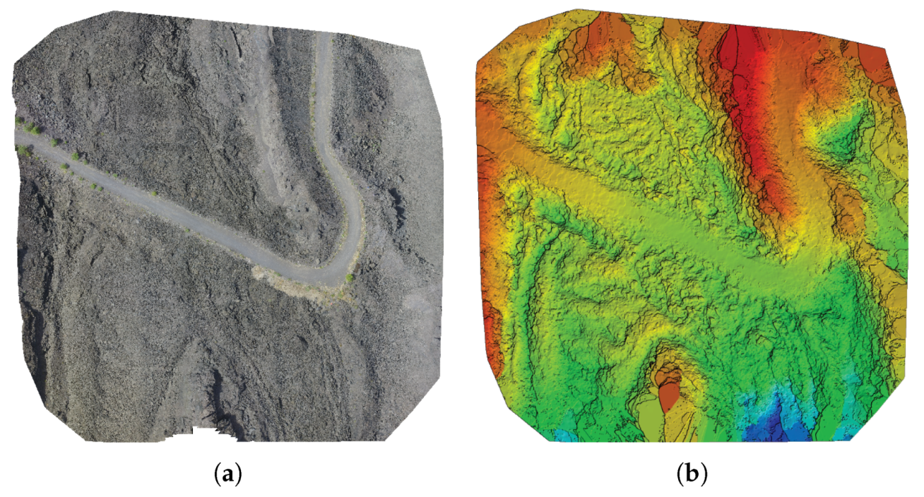
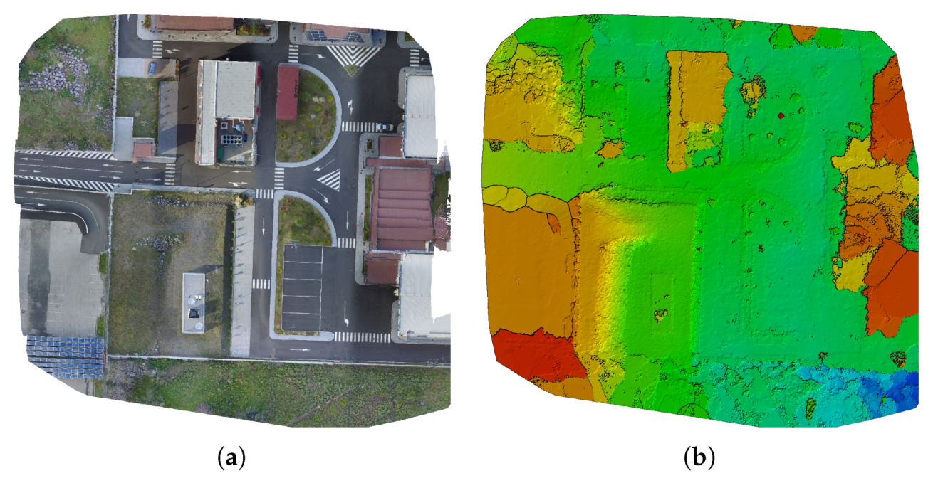
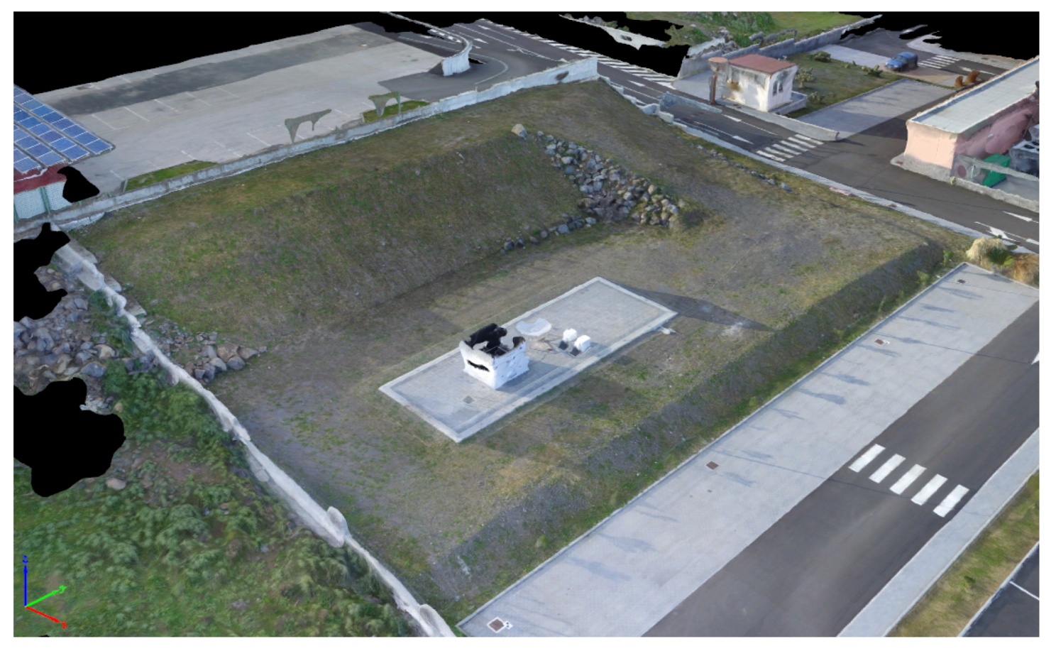
Regarding the landslide-like area, it is part of a semi-urban environment. We already had the 3D reconstruction of such an environment as we used it in previous works. It was still derived with Pix4Dmapper from the aerial imagery acquired a DJI Phantom 3 Pro platform during a 20 m-high survey mission. Also in that case on-field measured GCPs were introduced to enhance the georeferencing accuracy. In this case, the average GSD obtained was 0.98 cm/pixel. The related orthomosaic, DSM and the textured 3D mesh portion of the landslide-like area are represented in Figure 3 and Figure 4 respectively.
5. DSM Processing
The following data are derived from the DSM GeoTIFF file:
- a matrix, with the same size of the embedded raster image, where each element contains the encoded elevation value (in meters). In the remainder of this paper, we will refer to this matrix as elevation matrix;
- a structure that includes the geographical information (coordinates, datum and coordinate system), which are used to locate the elements of the elevation matrix and which will be used for georeferencing the generated trajectory.
The elevation matrix is processed by applying: (1) downsampling, (2) dilation, and (3) smoothing operators. Downsampling can be activated by the operator in the case of limited computational resources, as full-sized matrix processing could be excessively long. The downsampling step can be defined according to the final accuracy required by the application.
The dilation is a morphological image processing operation. It tends to thicken the boundaries of the objects in an image by using a structuring element. The shape and the size of such a structuring element define the number of pixels added to the boundaries [23]. Although it is primarily used in image processing, it can be also applied to DSMs as they can be treated as raster grayscale images. The grayscale dilation of image by structuring element , denoted by , is derived as [23]:
where is the structuring element’s domain, i.e., a binary matrix defining the neighborhood included in the operation. We assume outside the domain of the image. The structuring element values are added to the A values for each translated location and the maximum is derived. The main difference between classical convolution and grayscale dilation is that in the latter, for an arbitrary pair of coordinates in the domain , the term is included in the max computation only if . This is repeated for all coordinates , each time that coordinates change.
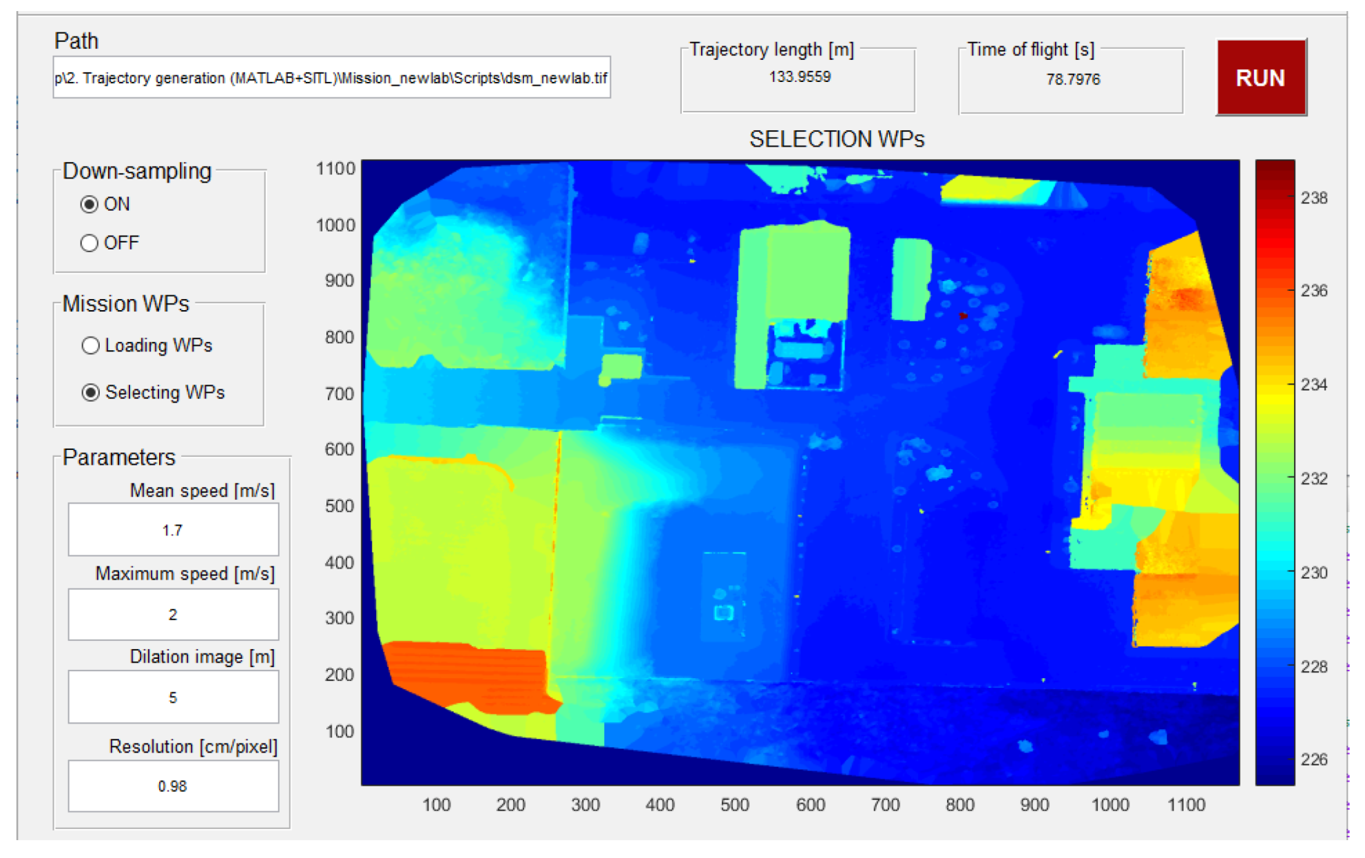
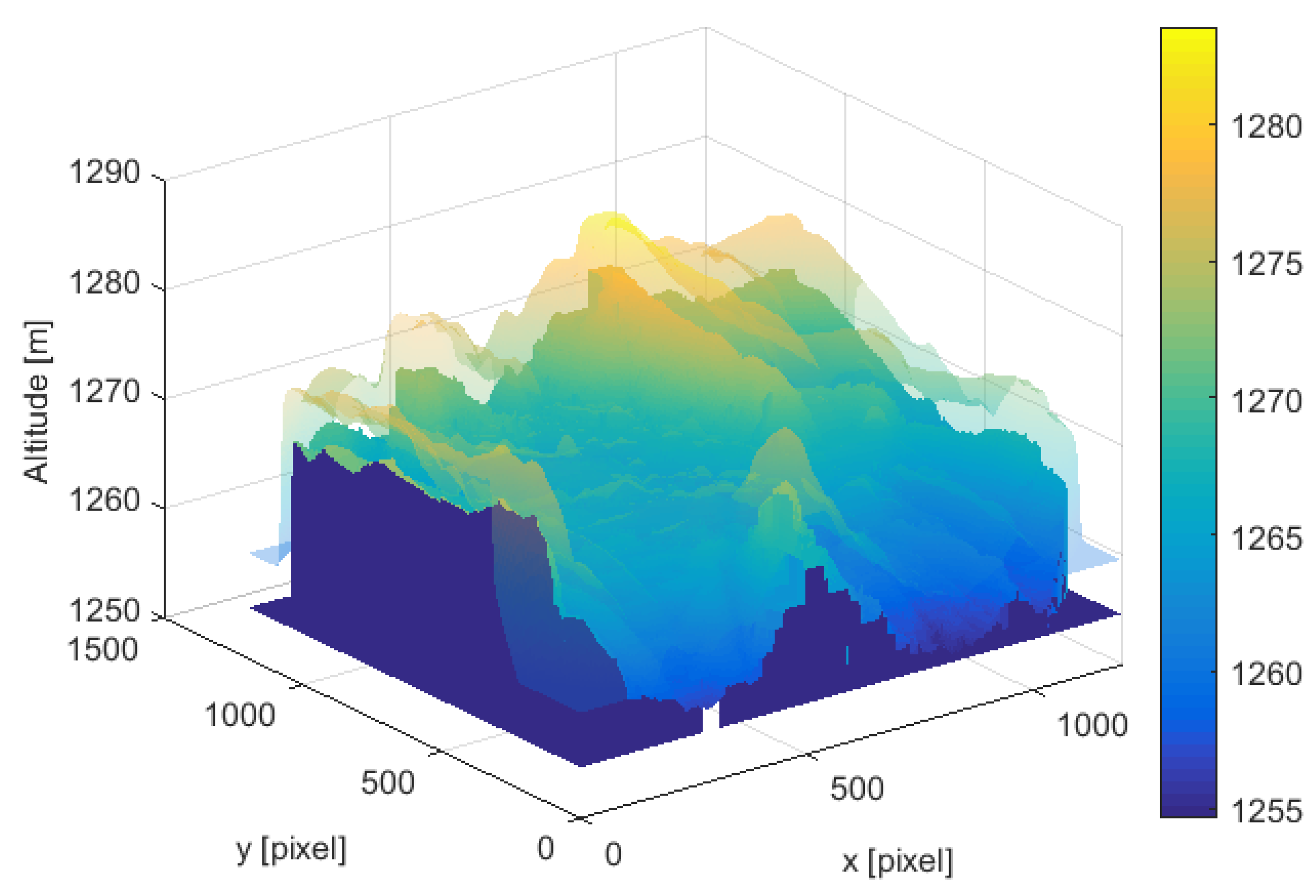
In our case, the dilation is performed by using a non-flat, ball-shaped structuring element, which is characterized by a radius R in the plane and an offset height H. When applied on the DSM, this operation implies an increase of the altitude values according to the ball height. This ensures a safe distance between the obstacles of the area of interest and the vehicle’s trajectory. Moreover, such an ellipsoidal shape allows us to avoid flying through narrow passages (e.g., urban or natural canyons) where the on-board GPS could have poor satellite visibility or may suffer from multipath effect, resulting in a poorly accurate localization. A graphical user interface was developed in Matlab (Figure 5) to easily handle the downsampling operation of the elevation matrix and to assign the parameters of the structuring element for the dilation operator. Finally, a Gaussian filter [23] is applied to smooth the DSM after the dilation. An example of the dilation and smoothing process applied on the volcanic area DSM is shown in Figure 6.
6. Trajectory Generation Procedure
This phase begins with the selection of the points of interest the UAV must approach during its flight. The GUI allows us to load the POI from a file or to select them by clicking on the map. The developed algorithm generates the trajectory taking into account the set of POI and the features of the DSM. We are assuming to employ a multirotor aerial vehicle, since this type of vehicles are particularly suited to perform detailed surveys as they can hover over a potential point of interest.
In our case, as we are interested in a low-altitude flight, the trajectory was computed as follows:
- the segment connecting two consecutive points of interest is created and then sampled with a sampling distance of 10 cm to obtain the coordinates, which are the latitude and longitude locations;
- for each coordinate the z coordinate (i.e., the flight height) is derived using the corresponding altitude of the dilated and smoothed DSM;
- a specified timing for the path execution is assigned by using a Linear Segment with Parabolic Blends (LSPB) trajectory, once fixed the mean and the maximum desired speed. For each waypoint, additional information concerning the loiter time (i.e., the time that the vehicle must stay flying over a WP before going to the next one) will be generated.
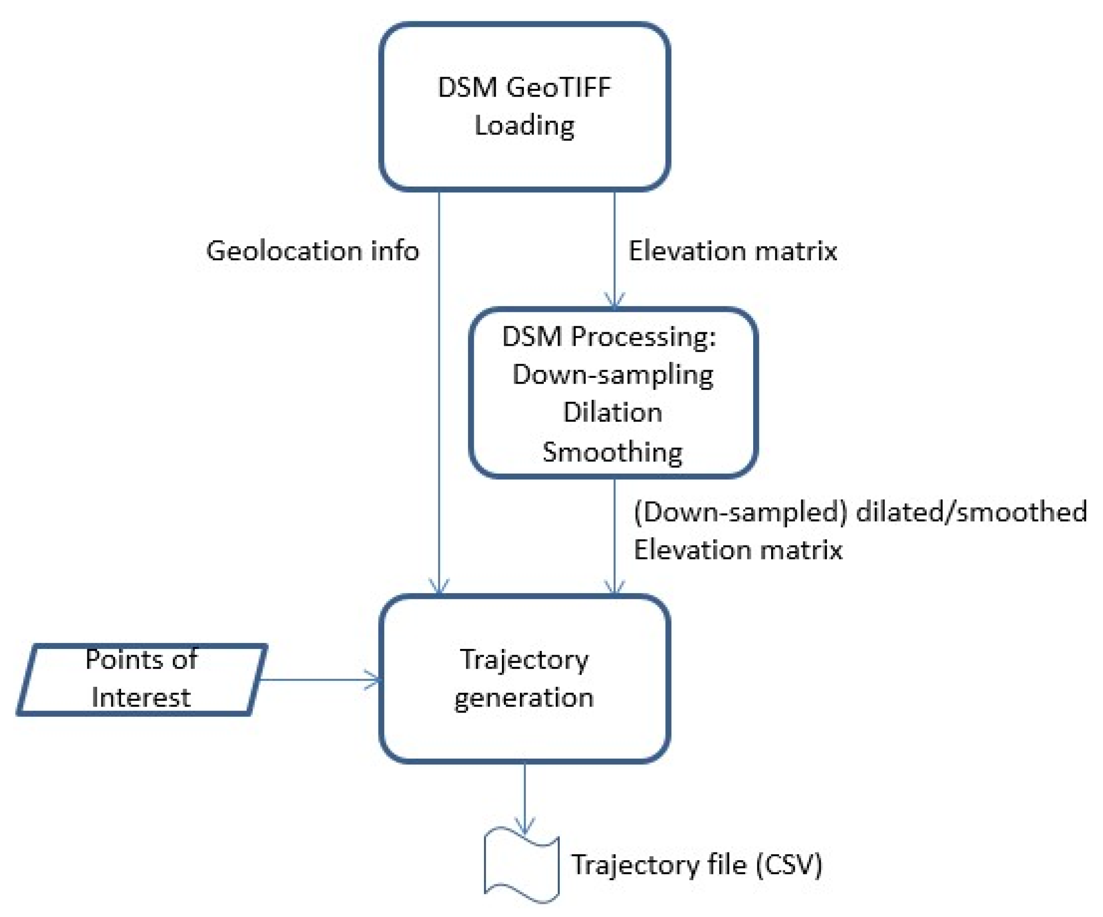
This strategy allows us to hedgehop, surfing on the dilated DSM, thus maintaining a safe distance from the ground and the obstacles. The computed trajectory is exported as a CSV text file in which the generated sequence of waypoints (WPs) is saved. Each waypoint has geographic coordinates (latitude, longitude, and altitude), groundspeed, and the time necessary to pass from one WP to the next. Moreover, a Keyhole Markup Language (KML) file is generated, containing only the locations of the WPs to verify them on Google Earth before starting the mission. To summarize, the workflow of the whole procedure from the original DSM up to the waypoints list is depicted in Figure 7.
Trajectory Generation Parameters
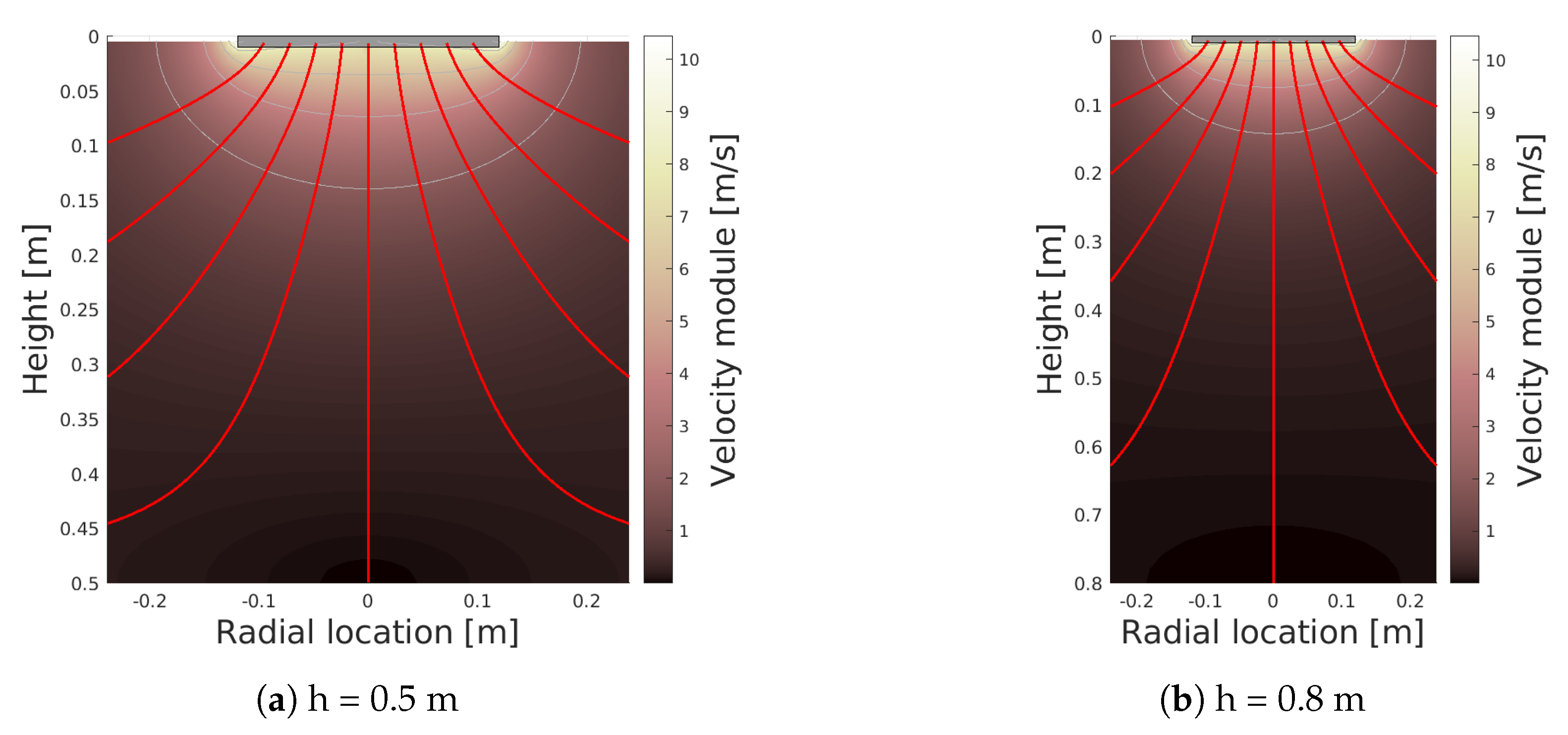
The radius (R) and the height (H) of the dilating element have to be appropriately chosen in order to guarantee a safe distance between the vehicle and both the obstacles and the terrain. Furthermore, when flying too close to the terrain, a multirotor may suffer from so-called ground effect. To avoid the flight in ground effect, we decided to estimate the downwash flow below rotor disk. To this end, a simulation of the rotors’ downwash was performed with the help of the model presented in [24], adapted for our setup. Each rotor disk of the UAV has a diameter of 24 cm and the induced velocity in hovering is assumed to be 5 m/s (in accordance with [25]). The results of two sample simulations are shown in Figure 8. From the simulations performed we found out the downwash wake of our rotors vanishes 0.5 m below rotor disk. Since in our case, the on-board GNSS receiver used for the low-altitude flight is a standalone (i.e., not RTK) device, with an accuracy of 2.5 m CEP (Circular Error Probable), we had to fly at an altitude at which the ground effect can be certainly neglected.
Once the downwash effect was excluded, the R and H parameters values were established by taking into account the accuracy of the reconstructed model (besides the accuracy of the vehicle’s localization system). As opposed to the UAV, the reconstructed surface models were precisely georeferenced with an accuracy of 0.023 m (mean RMS error) for both the volcanic environment and the landslide-like area. In the case of the lava flow reconstruction, this result was achieved thanks to the introduction of the four GCPs’ coordinates measured on field, as explained in Section 4.
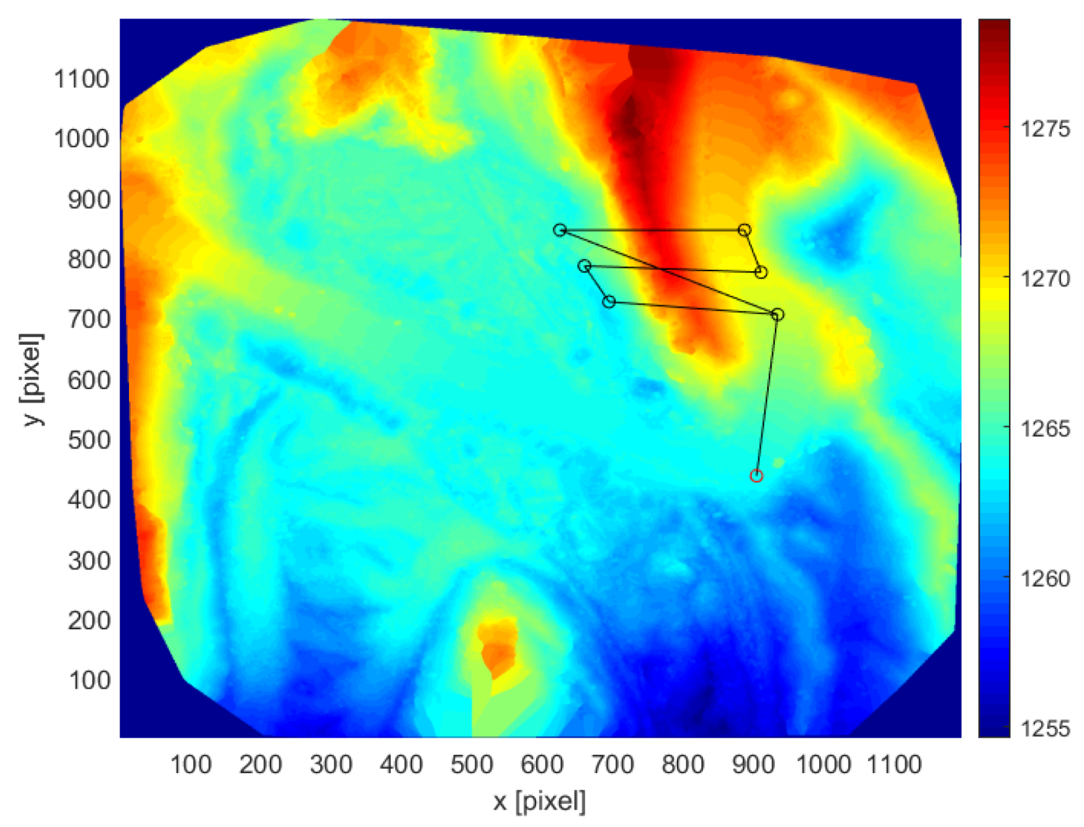
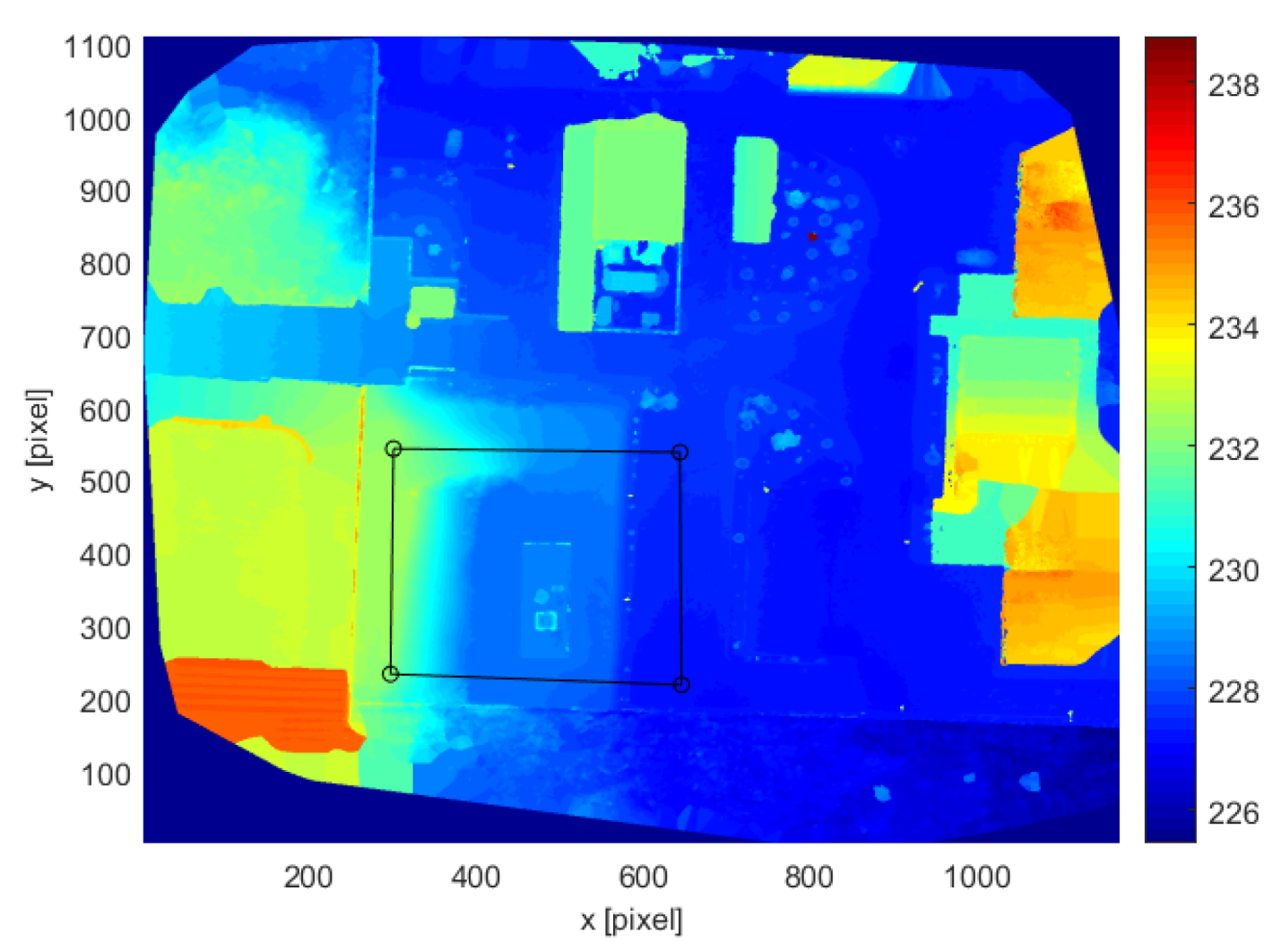
The selected POI for the volcanic scenario are indicated with circles in Figure 9, showing the color-coded DSM of the area. The points of interest are connected by the segments representing the 2D trajectory.
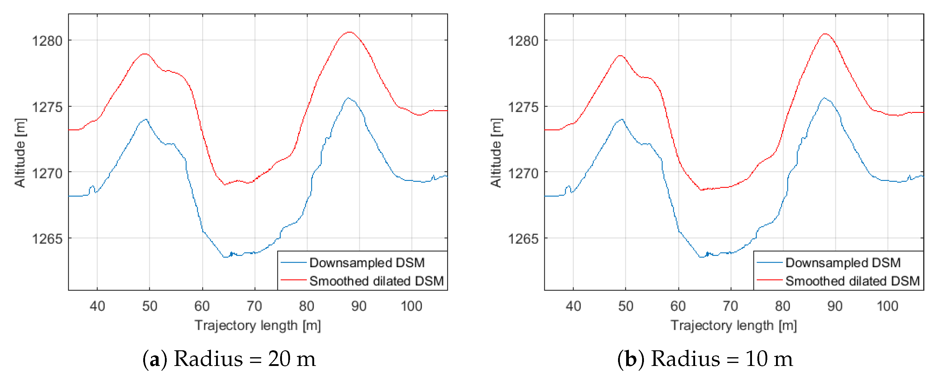
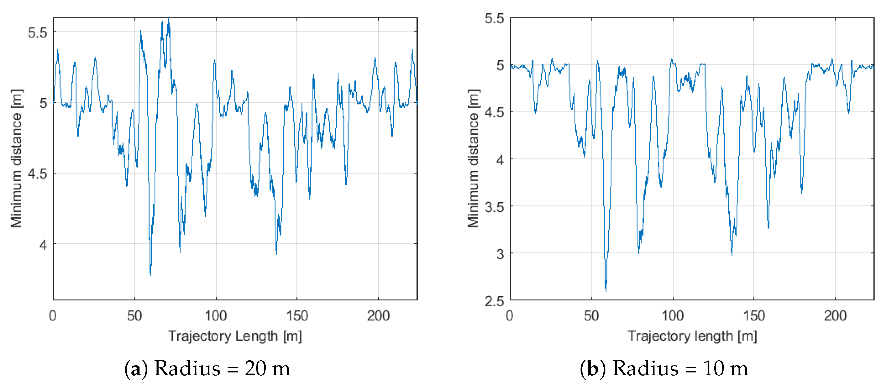
Figure 10a,b show portions of the altitude trends obtained for the selected POI and by applying the dilation operation with two structuring elements with the same height (5 m) but different radii. In the figure on the left, this value was set to 20 m, while on the right the results are obtained with a value of 10 m. It is possible to observe that in the second case the trajectory is generally closer to the terrain. This is even clearer from the plot reported in Figure 11 showing the minimum distance for each point of the computed trajectory to the DSM. A minimum distance of 3.80 m is observed when m, while this distance is only 2.59 m when m. From these observations, a ratio equal to four was determined to ensure a safe separation from the obstacles, both in the plane and in height, and the final H value was chosen equal to 5 m.
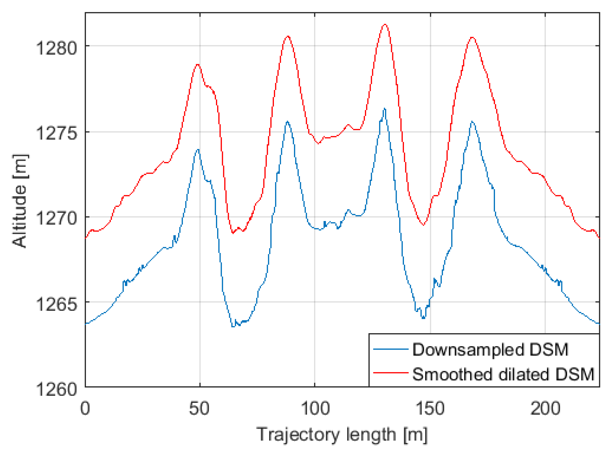
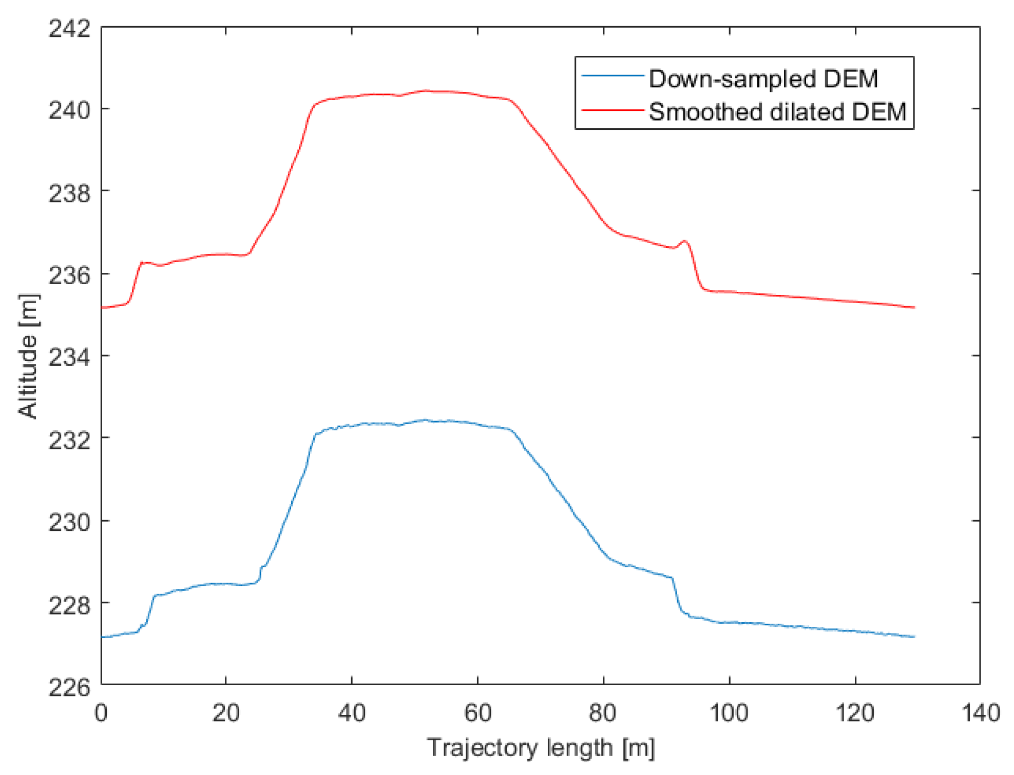
The lines of Figure 12 show the altitude trends with respect to the covered distance: the blue line follows the height of the original DSM; while the red line represents the reference altitude trend for the aerial vehicle resulting from the dilating/smoothing procedure. It is possible to observe that this trajectory maintains a safe distance from the obstacles and avoids flying through deep and narrow gorges as desired.
7. Experimental Setup
The solution was developed and tested by using a quadrotor based on a Flame Wheel 450 frame by DJI, equipped with a Pixhawk autopilot (https://pixhawk.org last accessed on 2020/06/14). This UAV was also used for the previous airborne imagery acquisition of the volcanic scenario. We decided to adopt the ArduPilot open-source software suite (http://ardupilot.org last accessed on 2020/06/14), which offers a complete and versatile control stack providing many flight modalities.
The MAVLink, Micro Air Vehicle Communication Protocol was used to communicate and interact with the autopilot over a serial connection. It is possible to retrieve all of the telemetry data (GPS, attitude, etc.), as well as to send commands to the autopilot.
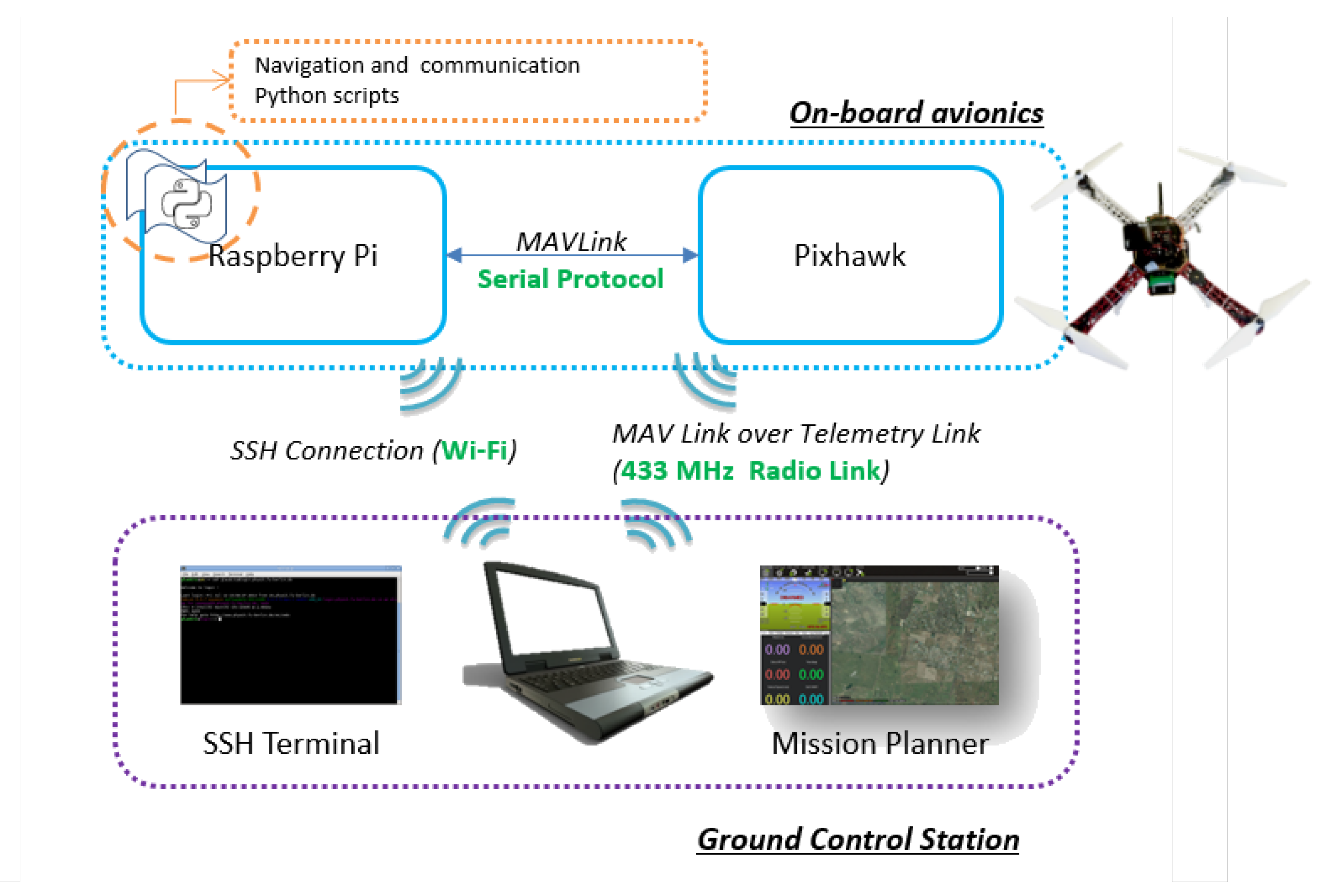
The setup adopted for the on-field tests is outlined in Figure 15. A Raspberry Pi 3B+, was used as an on-board companion computer. It implements the high-level navigation tasks through scripts communicating via MAVLink and sending the proper commands to the autopilot. The Raspberry communicates with the Ground Control Station (GCS) over a WiFi connection. Alternatively, it is possible to directly communicate from the GCS with the autopilot by using a dedicated 433 MHz radio link. The Mission Planner ground control interface allows us to setup and configure the autopilot, as well as to plan and manage all of the phases of a mission.
8. Software in the Loop Simulations
The script was tested with the Software in The Loop (SITL) copter simulation architecture by ArduPilot. The SITL simulator allows an executable of the ArduPilot firmware to run on a PC, in order to test the behavior of the system without using the real hardware (namely the autopilot and the vehicle). Moreover, the ArduPilot executable is connected to a flight simulator, implementing the flight dynamics. The executable sends a command to the flight simulator, which sends sensor data back to the emulated autopilot.
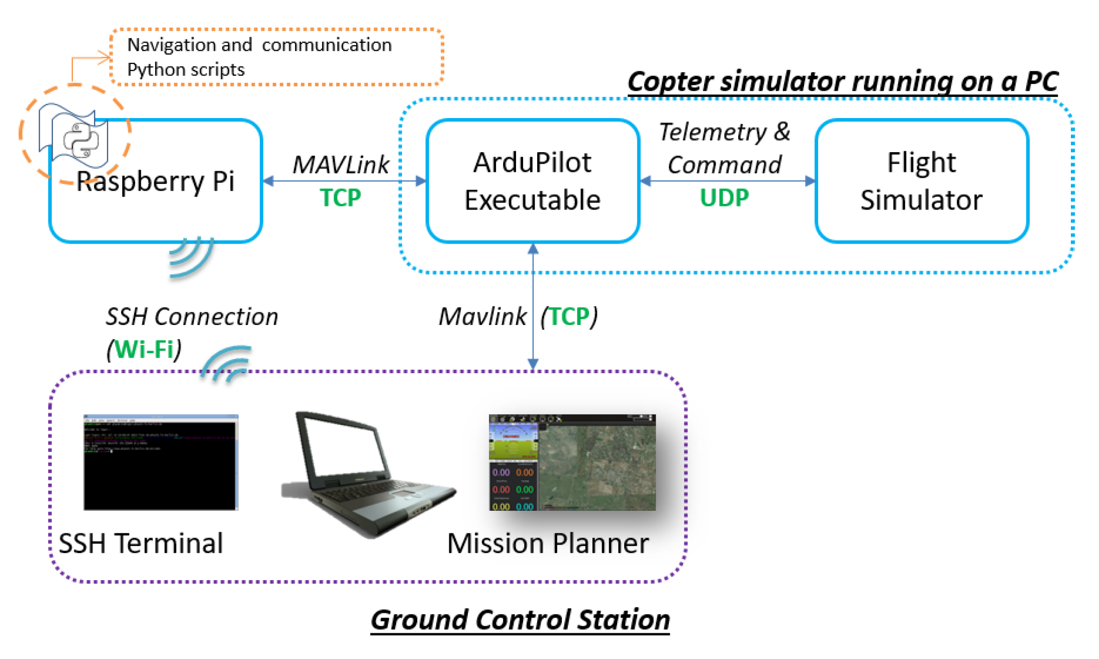
Figure 16 illustrates the setup used for the SITL simulations. In this case, the Raspberry Pi, running the script, is connected to the ArduPilot executable via MAVLink over TCP, thanks to the connection rerouting of Dronekit from serial. An internal UDP connection allows the data and command exchange between the ArduPilot executable and the flight simulator.
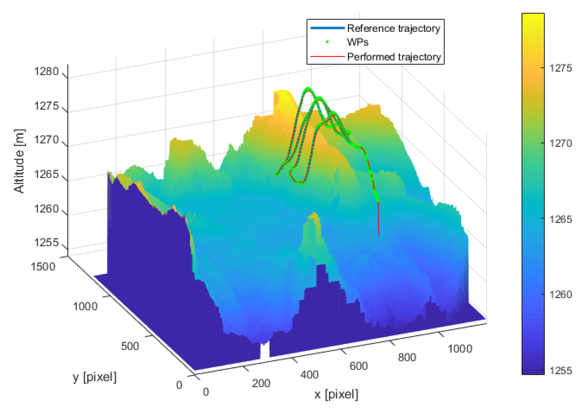
Figure 17 and Figure 18 show the results obtained using the SITL simulator: the trajectories are plotted over the DSM of the lava flow and the landslide-like area respectively. As can be observed, the performed trajectories are almost overlapped with the reference trajectory. This provided a first qualitative validation of the developed script before performing the on-field tests.
9. On-Field Tests and Results
Once we had tested the trajectory generation and the navigation script in simulation, the same script and trajectory were tested in the real testing scenarios by using the setup shown in Figure 15.
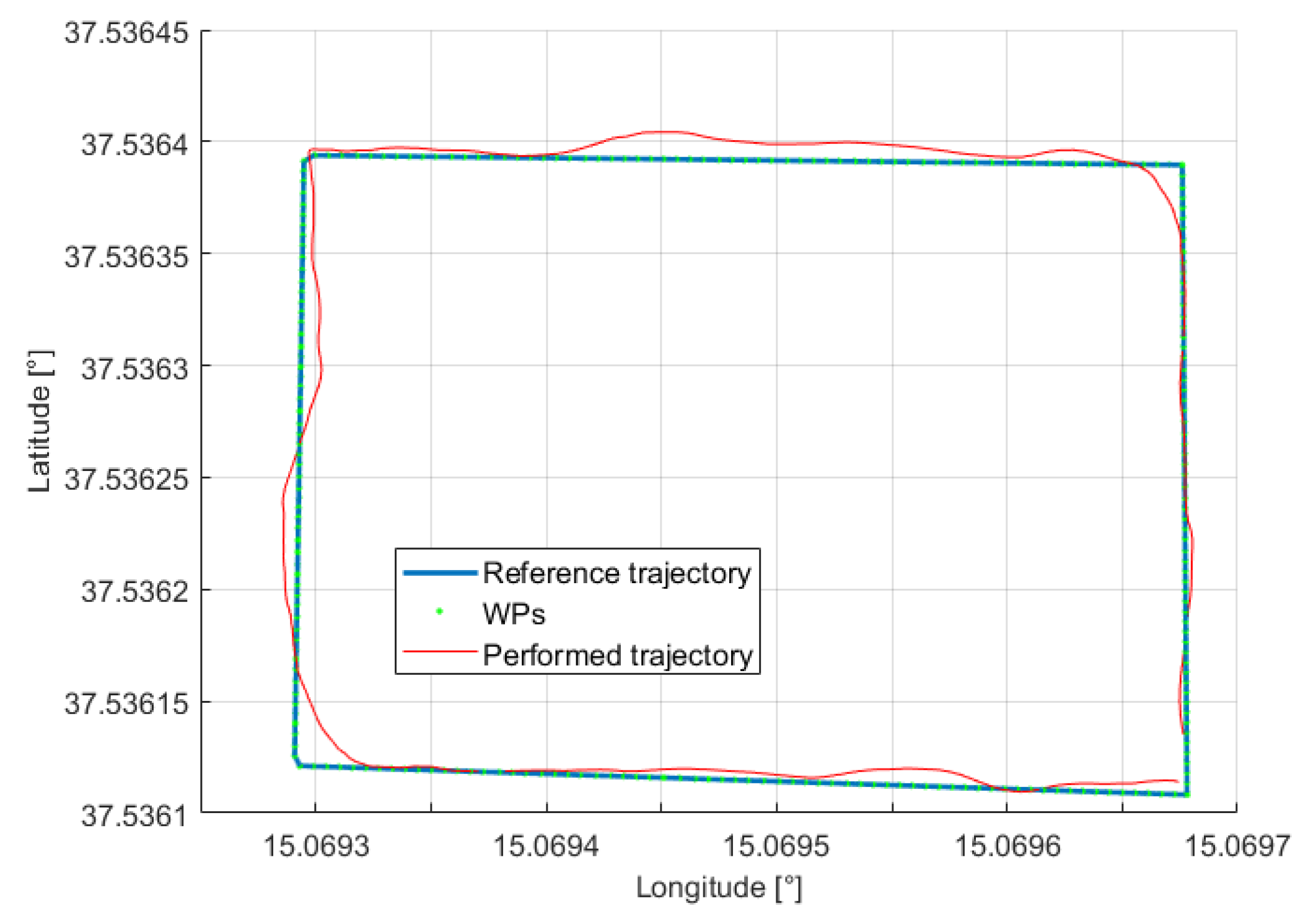
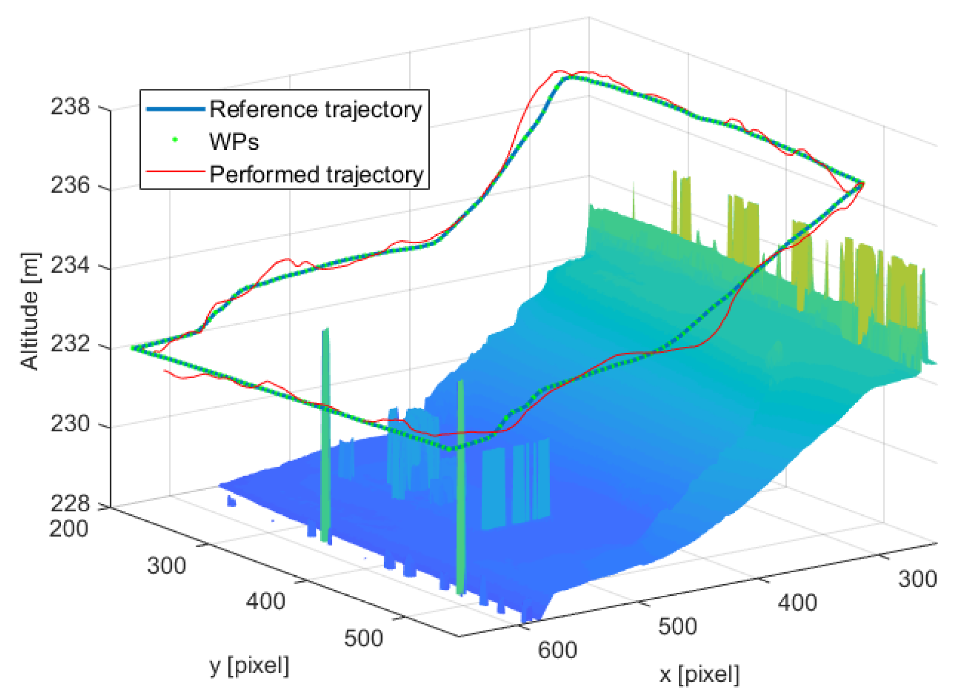
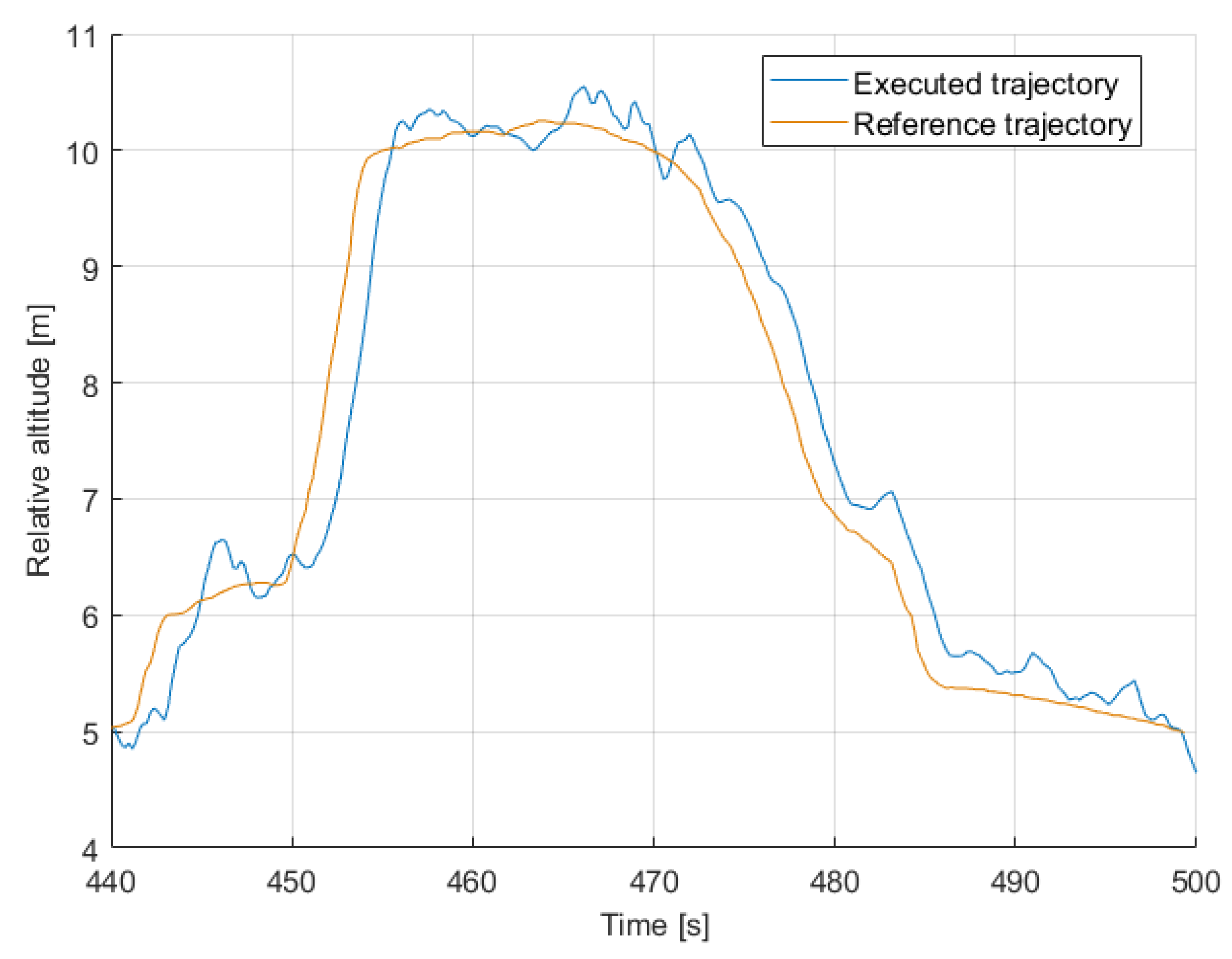
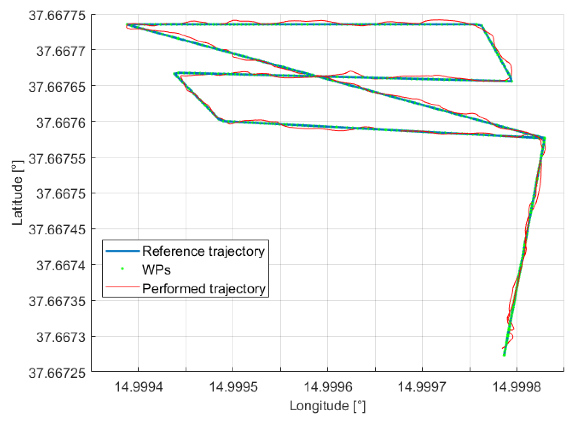
As already mentioned, a preliminary on-field trial was performed at the landslide-like area. In Figure 19 the executed trajectory, the reference trajectory and the obtained WPs projected on the longitude-latitude plane are shown. Figure 20 depicts the same trajectories and waypoints superimposed to the DSM, in order to show the terrain-following feature. The reference trajectory along with the executed trajectory (both expressed in terms of relative altitude) are plotted over time in Figure 21. As can be observed, the UAV follows the assigned reference path with a temporal shift between the two trends due to the time needed to reach the assigned WP.
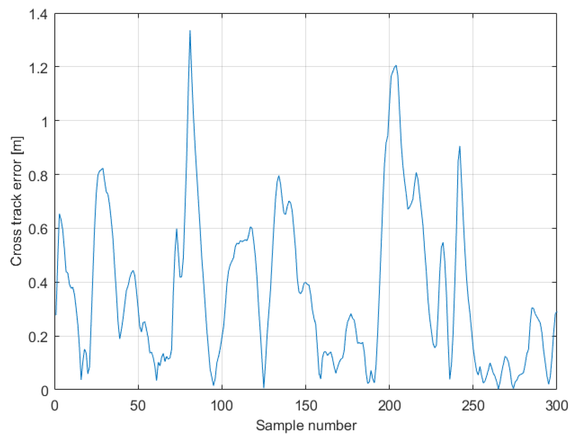
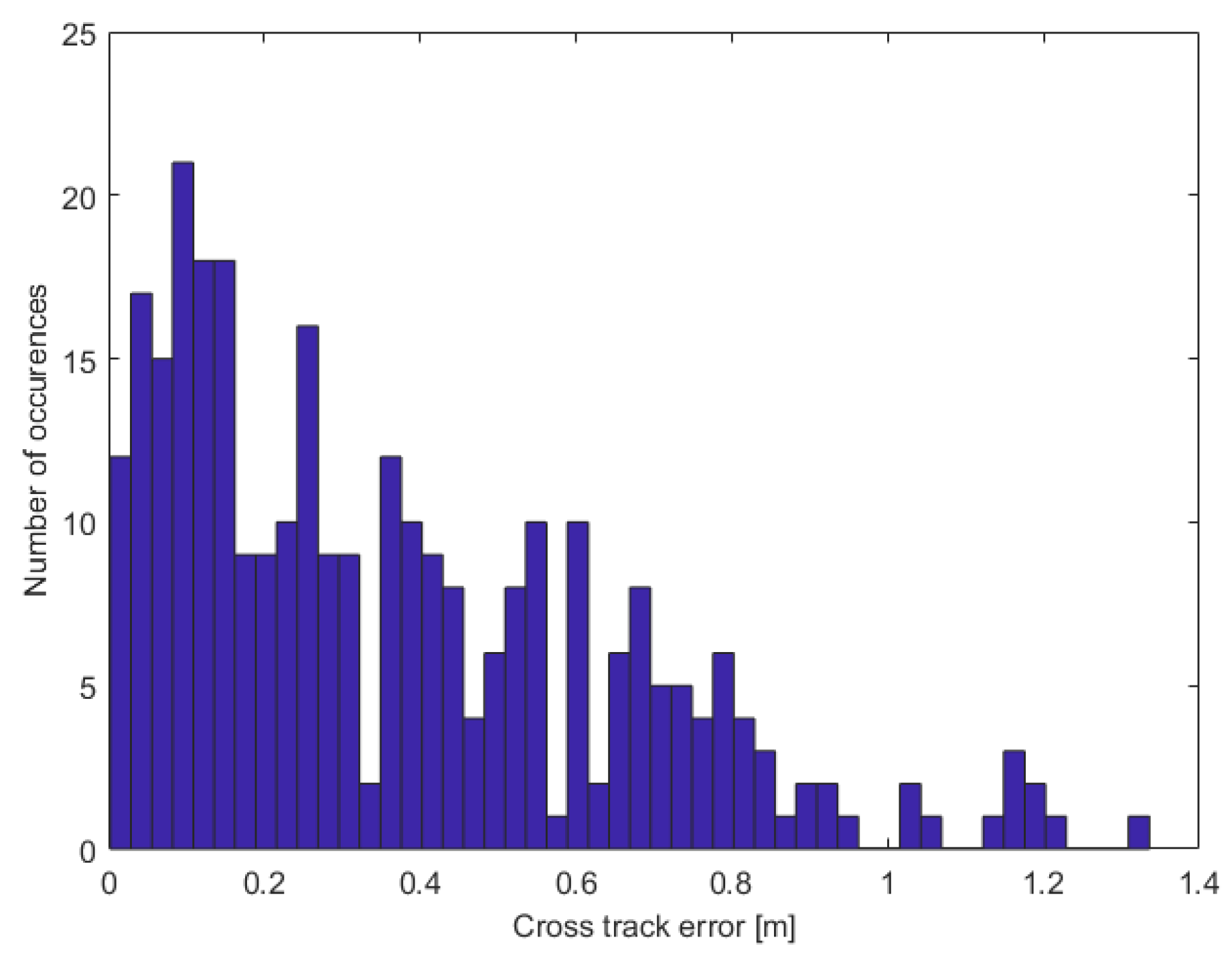
As a measure of the vehicle’s behavior we evaluated the cross track error, i.e., the distance from the desired route during the mission. Its trend and the related histogram are shown in Figure 22 and Figure 23, respectively. The maximum error observed is 1.37 m, which is still not a severe concern taking into consideration the safe distance included and the accuracy of the GPS system. It is anyway a rather high deviation from the desired trajectory. However, by observing the histogram it is possible to notice that the high error values (namely above 1 m) have fewer occurrences compared to the low values. This may highlight a local or temporary worsening in the localization system performance during the execution of the mission.
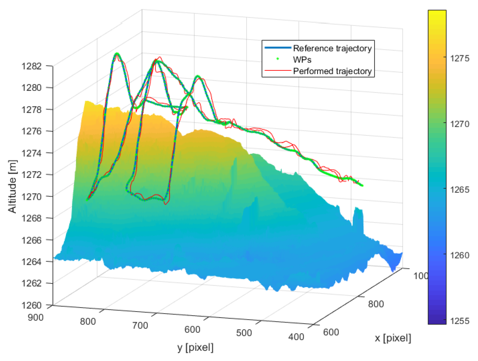
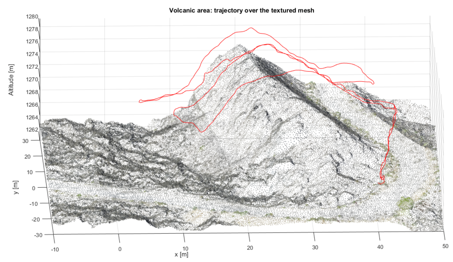
After the successful preliminary test, the second on-field testing at the Mount Etna volcano were carried out. Figure 24 shows again the projections of the executed trajectory, the reference trajectory and the obtained WPs on the longitude-latitude plane. In Figure 25 the same trajectories are plotted over the DSM. This last figure allows us to appreciate how the UAV follows the more complex morphology of the terrain (compared to the preliminary test) while flying close to the ground. Figure 26 shows in red the executed trajectory, plotted over the point cloud of the area.
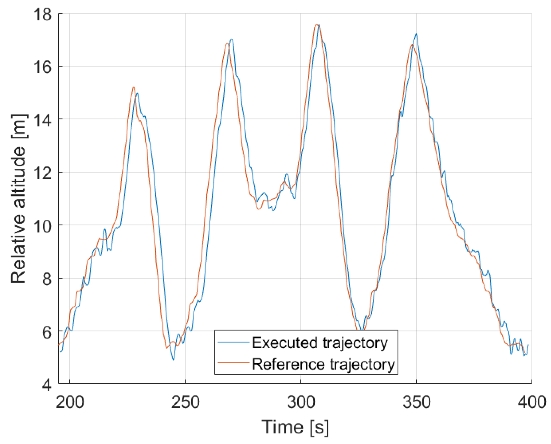
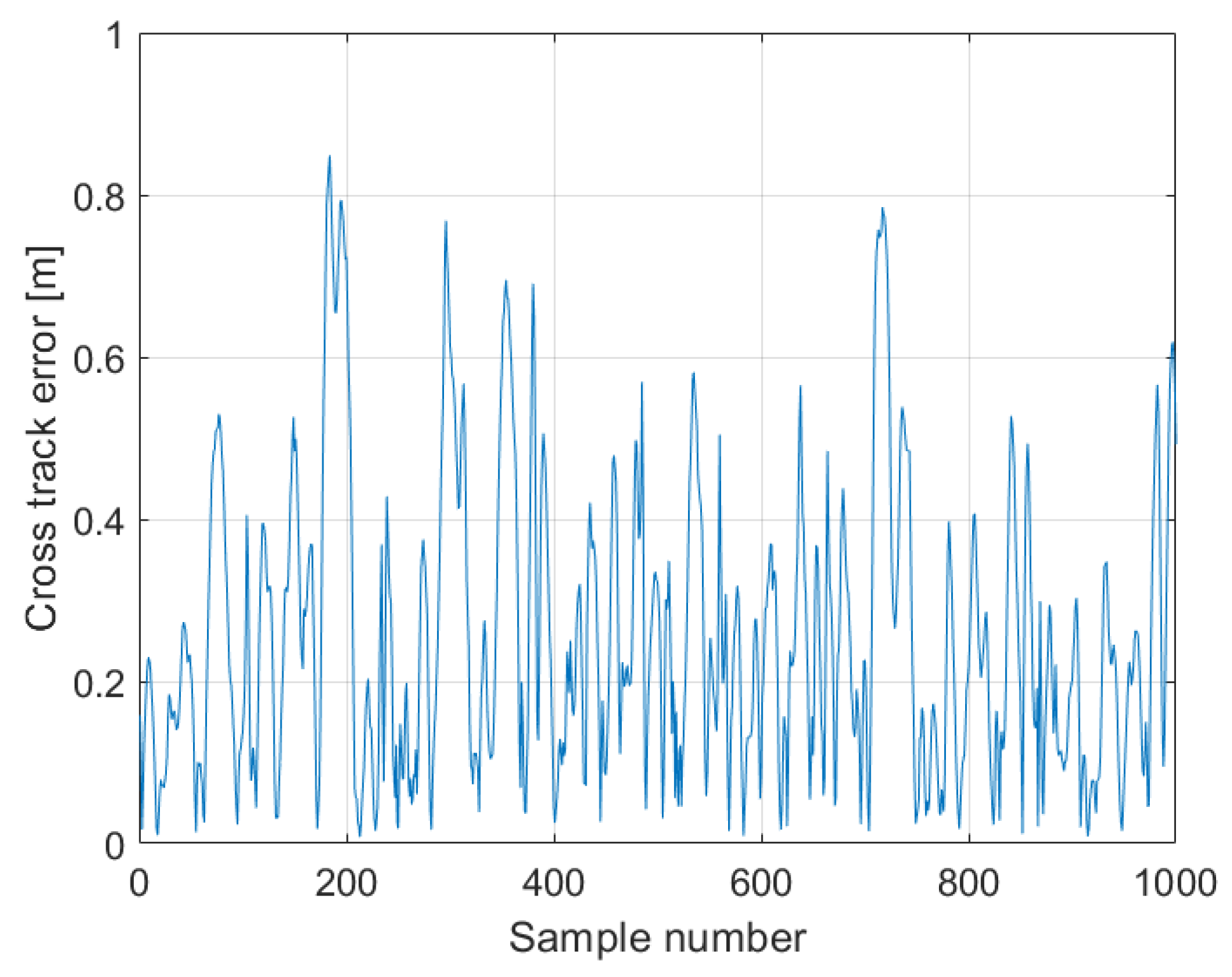
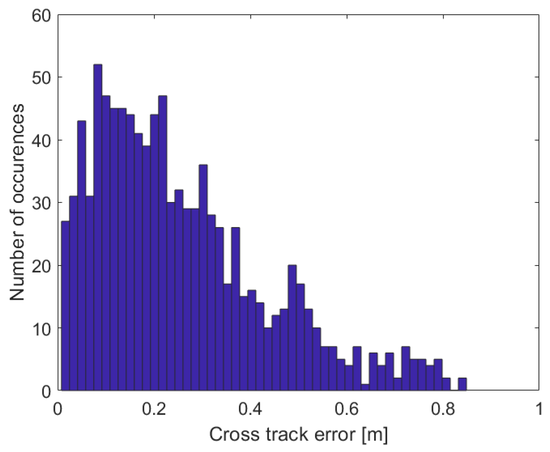
The plot of Figure 27 represents the relative altitude of the reference trajectory along with the trajectory of the executed mission against the mission time. Also in this case the temporal lag between the two trends can be observed. Figure 28 and Figure 29 represent the cross track error and its histogram, respectively. In this case, there is a maximum error of about 0.84 m. This represents a good performance, since it ensures a safe distance from the obstacles and ground, according to the errors in the localization. In general, the histogram shows that the values of the error are mostly between 0.1 and 0.3 m. This is a much better result compared to the one observed during the preliminary test.
We suppose the slightly worse performance in the landslide-like area is essentially related to the worse GPS localization performance, probably due to the presence of buildings in the surrounding zone. On the other hand, in the volcanic area we had an open field with no obstructions or buildings. This preliminary results call for a further statistical investigation on the GPS system behavior in different types of scenarios (urban, natural), weather conditions and, ideally, different geometries of the satellite constellation.
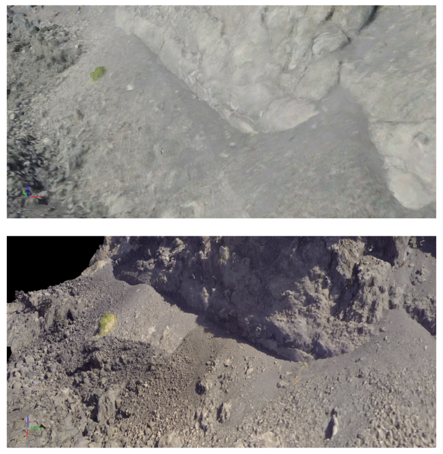
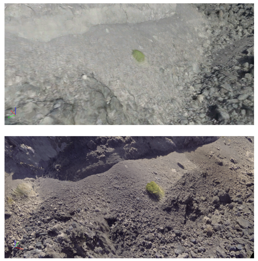
As an example of application, the images acquired during the low-altitude mission at the volcanic scenario were used as an input to Pix4Dmapper, in order to enhance the reconstruction quality of the 3D model of the area. The same processing options reported in Section 4 were used. However, ground control points could not be introduced in this case as they were not covered during the path execution of the mission and, hence, they were not acquired by the onboard camera. Figure 30 and Figure 31 show two details of the volcanic area as reconstructed by Pix4Dmapper by using the images acquired during the two survey flights at high and low altitude. The acquired data allows us to obtain a high-resolution 3D textured mesh that can be used for accurate measurements or for the identification of small objects, thus supporting the benefit of the proposed method.
The resulting average ground sampling distance is 1.36 cm/pixel. This value might appear worse than the one obtained with the 20 m-altitude flight (where we had GSD = 1.26 cm/pixel). However, it must be recalled that this is the average value derived by Pix4Dmapper for the whole DSM. Therefore, the higher GSD value for the 5 m-altitude flight, compared to the previous one, can be mainly ascribed to the poorly covered areas within the DSM matrix. In fact, this second reconstruction was carried out from the pictures acquired during the testing mission which was not a coverage mission. Moreover, the lack of ground control points worsen the georeferencing process by the mapping software and, as a consequence, the whole matching process. In summary, Pix4Dmapper was able to obtain a GSD for the 5 m-altitude flight which is comparable to the one previously achieved at 20 m, even without ground control points and by covering a much smaller area.
10. Conclusions and Future Work
This paper presents a method for multirotor flights close to the ground following the terrain profile and taking into account the uncertainties of both the environment DSM and the onboard GPS. As explained, this type of missions are extremely useful for the collection of imagery close to the ground, which have a wide spectrum of applications.
The proposed solution is versatile, including the assignment of a desired mean and maximum velocity to the survey mission. The computed trajectory is exported as a list of waypoints. In this manner, the mission can be imported in several commercial and open-source ground control stations and uploaded to almost all autopilots and multirotors.
The experimental missions confirmed the preliminary results obtained during the simulation and development phase. The vehicle always kept a safe distance from the terrain and the obstacles, even with a standard GPS localization system.
To summarize, the main contributions of this work are:
- generation of flights at lower altitudes compared to the solutions available for low-cost autopilots, including terrain awareness;
- desired velocity assignment for the survey mission, in accordance with the specificity of the mission and the vehicle’s performance;
- safety margin derivation after rotor downwash assessment;
- adoption of low-cost hardware.
One of the main limitations of our solution is related to the need for the surface model, which may require a long time through the photogrammetry software. This prevents our approach to be applied in situations where responsiveness is crucial. Another limiting aspect is related to the lack of robustness against potential severe failures of the GPS localization system or to dynamic changes of the environment. However, this limit may be overcome by providing the vehicle with range sensors and including a reactive-based local obstacle avoidance control as the ones discussed in [26]. Furthermore, the current solution was conceived and tested for multirotors only, as only this type of vehicles are able to perform the survey with a loiter time and, more generally, to hover above a specified target. Further investigation would be needed whether this solution should be adapted to other types of aerial vehicles (e.g., fixed wing). However, if no loiter time is needed, our solution may be applied to other vehicles as well.
Finally, moving to solutions for even lower altitudes, proper control strategies may be integrated as the one presented in [19], which may be enhanced with the terrain-following feature. A further enhancement to our solution could also be the integration of a prior assessment of the minimum distance between the computed trajectory and the DSM, according to the given radius of the structuring element of the dilation. This feature would provide a measure of the actual safe distance ensured throughout the mission execution.
Author Contributions
Conceptualization, C.D.M. and G.M.; Investigation, C.D.M., D.C.G. and L.C.; Methodology, C.D.M., D.C.G. and G.M.; Software, G.D.M. and I.M.; Supervision, G.M.; Writing—original draft, C.D.M.; Writing—review & editing, D.C.G. All authors have read and agreed to the published version of the manuscript.
Funding
This research has been partially supported by University of Catania under the project “Piano della Ricerca 2016-18. Linea intervento 2”.
Conflicts of Interest
The authors declare no conflicts of interest.
Abbreviations
The following abbreviations are used in this manuscript:
| AGL | Above Ground Level |
| DSM | Digital Surface Model |
| GCP | Ground Control Point |
| GCS | Ground Control Station |
| GNSS | Global Navigation Satellite System |
| GSD | Ground Sampling Distance |
| RTK | Real-Time Kinematic |
| UAV | Unmanned Aerial Vehicle |
| WP | Waypoint |
References
- Colomina, I.; Molina, P. Unmanned aerial systems for photogrammetry and remote sensing: A review. ISPRS J. Photogramm. Remote. Sens. 2014, 92, 79–97. [Google Scholar] [CrossRef] [Green Version]
- Nex, F.; Remondino, F. UAV for 3D mapping applications: A review. Appl. Geomat. 2014, 6, 1–15. [Google Scholar] [CrossRef]
- Melita, C.D.; Longo, D.; Muscato, G.; Giudice, G. Measurement and Exploration in Volcanic Environments. In Handbook of Unmanned Aerial Vehicles; Springer: Berlin/Heidelberg, Germany, 2015; pp. 2667–2692. [Google Scholar]
- Niethammer, U.; James, M.; Rothmund, S.; Travelletti, J.; Joswig, M. UAV-based remote sensing of the Super-Sauze landslide: Evaluation and results. Eng. Geol. 2012, 128, 2–11. [Google Scholar] [CrossRef]
- Achille, C.; Adami, A.; Chiarini, S.; Cremonesi, S.; Fassi, F.; Fregonese, L.; Taffurelli, L. UAV-based photogrammetry and integrated technologies for architectural applications-Methodological strategies for the after-quake survey of vertical structures in Mantua (Italy). Sensors 2015, 15, 15520–15539. [Google Scholar] [CrossRef] [PubMed] [Green Version]
- Immerzeel, W.; Kraaijenbrink, P.; Shea, J.; Shrestha, A.; Pellicciotti, F.; Bierkens, M.; De Jong, S. High-resolution monitoring of Himalayan glacier dynamics using unmanned aerial vehicles. Remote. Sens. Environ. 2014, 150, 93–103. [Google Scholar] [CrossRef]
- Qi, J.; Song, D.; Shang, H.; Wang, N.; Hua, C.; Wu, C.; Qi, X.; Han, J. Search and rescue rotary-wing UAV and its application to the Lushan Ms 7.0 earthquake. J. Field Robot. 2016, 33, 290–321. [Google Scholar] [CrossRef]
- Duncan, B.A.; Murphy, R.R. Comparison of flight paths from fixed-wing and rotorcraft small unmanned aerial systems at SR530 mudslide Washington state. In Proceedings of the 2015 IEEE International Conference on Robotics and Automation (ICRA), Seattle, WA, USA, 26–30 May 2015; pp. 3416–3421. [Google Scholar]
- Murphy, R.R.; Duncan, B.A.; Collins, T.; Kendrick, J.; Lohman, P.; Palmer, T.; Sanborn, F. Use of a Small Unmanned Aerial System for the SR-530 Mudslide Incident near Oso, Washington. J. Field Robot. 2016, 33, 476–488. [Google Scholar] [CrossRef] [Green Version]
- Grasso, V.F.; Singh, A.; Pathak, J. Early Warning Systems: State-of-Art Analysis and Future Directions; Technical Report; Division of Early Warning and Assessment (DEWA); United Nations Environment Programme (UNEP): Nairobi, Kenya, 2012. [Google Scholar]
- Pajares, G. Overview and current status of remote sensing applications based on unmanned aerial vehicles (UAVs). Photogramm. Eng. Remote. Sens. 2015, 81, 281–330. [Google Scholar] [CrossRef] [Green Version]
- Nissen, E.; Krishnan, A.K.; Arrowsmith, J.R.; Saripalli, S. Three-dimensional surface displacements and rotations from differencing pre-and post-earthquake LiDAR point clouds. Geophys. Res. Lett. 2012, 39. [Google Scholar] [CrossRef]
- Stumpf, A.; Malet, J.P.; Kerle, N.; Niethammer, U.; Rothmund, S. Image-based mapping of surface fissures for the investigation of landslide dynamics. Geomorphology 2013, 186, 12–27. [Google Scholar] [CrossRef] [Green Version]
- Jin, X.; Liu, S.; Baret, F.; Hemerlé, M.; Comar, A. Estimates of plant density of wheat crops at emergence from very low altitude UAV imagery. Remote. Sens. Environ. 2017, 198, 105–114. [Google Scholar] [CrossRef] [Green Version]
- Reza, M.N.; Na, I.S.; Baek, S.W.; Lee, K.H. Rice yield estimation based on K-means clustering with graph-cut segmentation using low-altitude UAV images. Biosyst. Eng. 2019, 177, 109–121. [Google Scholar] [CrossRef]
- Zufferey, J.C.; Beyeler, A.; Floreano, D. Autonomous flight at low altitude with vision-based collision avoidance and GPS-based path following. In Proceedings of the 2010 IEEE International Conference on Robotics and Automation, Anchorage, AK, USA, 3–7 May 2010; pp. 3329–3334. [Google Scholar]
- Campos, I.S.; Nascimento, E.R.; Freitas, G.M.; Chaimowicz, L. A height estimation approach for terrain following flights from monocular vision. Sensors 2016, 16, 2071. [Google Scholar] [CrossRef] [Green Version]
- González, V.; Monje, C.; Moreno, L.; Balaguer, C. UAVs mission planning with flight level constraint using Fast Marching Square Method. Robot. Auton. Syst. 2017, 94, 162–171. [Google Scholar] [CrossRef]
- Chen, Y.; Zhang, G.; Zhuang, Y.; Hu, H. Autonomous flight control for multi-rotor UAVs flying at low altitude. IEEE Access 2019, 7, 42614–42625. [Google Scholar] [CrossRef]
- Johnson, E.N.; Mooney, J.G. A comparison of automatic nap-of-the-earth guidance strategies for helicopters. J. Field Robot. 2014, 31, 637–653. [Google Scholar] [CrossRef]
- Küng, O.; Strecha, C.; Beyeler, A.; Zufferey, J.C.; Floreano, D.; Fua, P.; Gervaix, F. The Accuracy of Automatic Photogrammetric Techniques on Ultra-Light UAV Imagery; UAV-g 2011—Unmanned Aerial Vehicle in Geomatics: Zürich, Switzerland, 2011. [Google Scholar]
- Harwin, S.; Lucieer, A. Assessing the accuracy of georeferenced point clouds produced via multi-view stereopsis from unmanned aerial vehicle (UAV) imagery. Remote. Sens. 2012, 4, 1573–1599. [Google Scholar] [CrossRef] [Green Version]
- Gonzalez, R.C.; Woods, R.E.; Eddins, S.L. Digital Image Processing Using Matlab; Pearson Prentice Hall: Upper Saddle River, NJ, USA, 2004. [Google Scholar]
- Hooi, C.G.; Lagor, F.D.; Paley, D.A. Height estimation and control of rotorcraft in ground effect using spatially distributed pressure sensing. J. Am. Helicopter Soc. 2016, 61, 1–14. [Google Scholar] [CrossRef] [Green Version]
- Bristeau, P.J.; Martin, P.; Salaün, E.; Petit, N. The role of propeller aerodynamics in the model of a quadrotor UAV. In Proceedings of the 2009 European Control Conference (ECC), Budapest, Hungary, 23–26 August 2009; pp. 683–688. [Google Scholar]
- Berger, C.; Rudol, P.; Wzorek, M.; Kleiner, A. Evaluation of reactive obstacle avoidance algorithms for a quadcopter. In Proceedings of the 14th International Conference on Control, Automation, Robotics and Vision (ICARCV), Phuket, Thailand, 13–15 November 2016; pp. 1–6. [Google Scholar]
Figure 1.
(a) Reconstructed orthomosaic and (b) DSM of the volcanic area on Mount Etna (area covered 0.0209 km, av. GSD = 1.26 cm/pixel).
Figure 1.
(a) Reconstructed orthomosaic and (b) DSM of the volcanic area on Mount Etna (area covered 0.0209 km, av. GSD = 1.26 cm/pixel).

Figure 2.
Textured 3D mesh of the lava flow.

Figure 3.
(a) Reconstructed orthomosaic and (b) DSM of the landslide-like area (area covered 0.0114 km, av. GSD = 0.98 cm/pixel).
Figure 3.
(a) Reconstructed orthomosaic and (b) DSM of the landslide-like area (area covered 0.0114 km, av. GSD = 0.98 cm/pixel).

Figure 4.
Textured 3D mesh of the semi-urban environment.

Figure 5.
The graphical user interface adopted to process the DSM and to generate the trajectory, including the considered color-coded DSM.
Figure 5.
The graphical user interface adopted to process the DSM and to generate the trajectory, including the considered color-coded DSM.

Figure 6.
Resulting smoothed and dilated DSM (faded) superimposed upon the downsampled DSM (solid).

Figure 7.
Flow chart of the proposed trajectory generation approach, from the original DSM up to the waypoints list.
Figure 7.
Flow chart of the proposed trajectory generation approach, from the original DSM up to the waypoints list.

Figure 8.
Downwash simulations of a UAV rotor at different altitudes according to the model in [24]. The gray rectangle depicts the side view of rotor disk.
Figure 8.
Downwash simulations of a UAV rotor at different altitudes according to the model in [24]. The gray rectangle depicts the side view of rotor disk.

Figure 9.
Computed trajectory (black line) for the selected points of interest in the volcanic area.
Figure 9.
Computed trajectory (black line) for the selected points of interest in the volcanic area.

Figure 10.
Volcanic area: details of the altitude trends obtained with two different values of the structuring element radius in the dilation operator.
Figure 10.
Volcanic area: details of the altitude trends obtained with two different values of the structuring element radius in the dilation operator.

Figure 11.
Volcanic area: minimum distance trends from the downsampled DSM for the two altitude trends in Figure 10.
Figure 11.
Volcanic area: minimum distance trends from the downsampled DSM for the two altitude trends in Figure 10.

Figure 12.
The altitude trends versus the covered distance for the volcanic area: in red the computed reference trajectory for the UAV, in blue the altitude trend of the downsampled DSM representing the terrain.
Figure 12.
The altitude trends versus the covered distance for the volcanic area: in red the computed reference trajectory for the UAV, in blue the altitude trend of the downsampled DSM representing the terrain.

Figure 13.
Computed trajectory (black line) for the selected points of interest in the landslide-like area.
Figure 13.
Computed trajectory (black line) for the selected points of interest in the landslide-like area.

Figure 14.
The altitude trends versus the covered distance for the landslide-like area: in red the computed reference trajectory for the UAV, in blue the altitude trend of the downsampled DSM representing the terrain.
Figure 14.
The altitude trends versus the covered distance for the landslide-like area: in red the computed reference trajectory for the UAV, in blue the altitude trend of the downsampled DSM representing the terrain.

Figure 15.
Setup used for the on-field tests.

Figure 16.
The architecture implemented for SITL simulations.

Figure 17.
SITL simulations—volcanic area: the reference trajectory (blue line), the WPs of the reference trajectory (green points) and the performed trajectory (red line) of the executed simulation are shown over the DSM.
Figure 17.
SITL simulations—volcanic area: the reference trajectory (blue line), the WPs of the reference trajectory (green points) and the performed trajectory (red line) of the executed simulation are shown over the DSM.

Figure 18.
SITL simulations—landslide-like area: the reference trajectory (blue line), the WPs of the reference trajectory (green points) and the performed trajectory (red line) of the executed simulation are shown over the DSM.
Figure 18.
SITL simulations—landslide-like area: the reference trajectory (blue line), the WPs of the reference trajectory (green points) and the performed trajectory (red line) of the executed simulation are shown over the DSM.

Figure 19.
Preliminary on-field test—landslide-like area: performed trajectory (in red) and reference path (in blue), together with the assigned waypoints (in green) in the longitude-latitude plane.
Figure 19.
Preliminary on-field test—landslide-like area: performed trajectory (in red) and reference path (in blue), together with the assigned waypoints (in green) in the longitude-latitude plane.

Figure 20.
Preliminary on-field test—landslide-like area: a detail of the trajectories plotted over the DSM of the area.
Figure 20.
Preliminary on-field test—landslide-like area: a detail of the trajectories plotted over the DSM of the area.

Figure 21.
Preliminary on-field test—landslide-like area: altitudes of the reference path (in red) and of the executed trajectory (in blue).
Figure 21.
Preliminary on-field test—landslide-like area: altitudes of the reference path (in red) and of the executed trajectory (in blue).

Figure 22.
Preliminary on-field test—landslide-like area: the cross track error values during the mission.
Figure 22.
Preliminary on-field test—landslide-like area: the cross track error values during the mission.

Figure 23.
Preliminary on-field test—landslide-like area: histogram of the cross track error.

Figure 24.
On-field test—volcanic scenario: performed trajectory (in red) and reference path (in blue), together with the assigned waypoints (in green) in the longitude-latitude plane.
Figure 24.
On-field test—volcanic scenario: performed trajectory (in red) and reference path (in blue), together with the assigned waypoints (in green) in the longitude-latitude plane.

Figure 25.
On-field test—volcanic scenario: a detail of the trajectories plotted over the DSM of the area.
Figure 25.
On-field test—volcanic scenario: a detail of the trajectories plotted over the DSM of the area.

Figure 26.
On-field test—volcanic scenario: a detail of the executed trajectory plotted over the point cloud of the area.
Figure 26.
On-field test—volcanic scenario: a detail of the executed trajectory plotted over the point cloud of the area.

Figure 27.
On-field test—volcanic scenario: altitudes of the reference path (in red) and of the executed trajectory (in blue).
Figure 27.
On-field test—volcanic scenario: altitudes of the reference path (in red) and of the executed trajectory (in blue).

Figure 28.
On-field test—volcanic scenario: the cross track error values during the mission.

Figure 29.
On-field test—volcanic scenario: histogram of the cross track error.

Figure 30.
On-field test: a visual comparison of the 3D meshes of the lava flow reconstructed by Pix4D mapper. The image on the top shows the results obtained by using the images acquired during the first flight, at high altitude (20 m). The image at the bottom shows the same area reconstructed by using the images acquired during the flight at low altitude (5 m).

Figure 31.
On-field test: a comparison of the 3D meshes of the lava flow reconstructed by Pix4D mapper. The image on the top shows the results obtained by using the images acquired during the first flight, at high altitude (20 m). The image at the bottom shows the same area reconstructed by using the images acquired during the flight at low altitude (5 m).

© 2020 by the authors. Licensee MDPI, Basel, Switzerland. This article is an open access article distributed under the terms and conditions of the Creative Commons Attribution (CC BY) license (http://creativecommons.org/licenses/by/4.0/).
Share and Cite
MDPI and ACS Style
Melita, C.D.; Guastella, D.C.; Cantelli, L.; Di Marco, G.; Minio, I.; Muscato, G. Low-Altitude Terrain-Following Flight Planning for Multirotors. Drones 2020, 4, 26. https://doi.org/10.3390/drones4020026
AMA Style
Melita CD, Guastella DC, Cantelli L, Di Marco G, Minio I, Muscato G. Low-Altitude Terrain-Following Flight Planning for Multirotors. Drones. 2020; 4(2):26. https://doi.org/10.3390/drones4020026
Chicago/Turabian StyleMelita, Carmelo Donato, Dario Calogero Guastella, Luciano Cantelli, Giuseppe Di Marco, Irene Minio, and Giovanni Muscato. 2020. "Low-Altitude Terrain-Following Flight Planning for Multirotors" Drones 4, no. 2: 26. https://doi.org/10.3390/drones4020026