Article

Elasmobranch Use of Nearshore Estuarine Habitats Responds to Fine-Scale, Intra-Seasonal Environmental Variation: Observing Coastal Shark Density in a Temperate Estuary Utilizing Unoccupied Aircraft Systems (UAS)

by
Alexandra E. DiGiacomo
*,
Walker E. Harrison
,
David W. Johnston
and
Justin T. Ridge
Duke University Marine Laboratory, Division of Marine Science and Conservation, Nicholas School of the Environment, Duke University, 135 Duke Marine Lab Rd, Beaufort, NC 28516, USA
*
Author to whom correspondence should be addressed.
Drones 2020, 4(4), 74; https://doi.org/10.3390/drones4040074
Submission received: 26 November 2020 / Revised: 3 December 2020 / Accepted: 5 December 2020 / Published: 8 December 2020
(This article belongs to the Special Issue Drone Technology for Wildlife and Human Management)

Abstract

:
Many coastal shark species are known to use estuaries of the coastal southeastern United States for essential purposes like foraging, reproducing, and protection from predation. Temperate estuarine landscapes, such as the Rachel Carson Reserve (RCR) in Beaufort, NC, are dynamic habitat mosaics that experience fluctuations in physical and chemical oceanographic properties on various temporal and spatial scales. These patterns in abiotic conditions play an important role in determining species movement. The goal of this study was to understand the impact of environmental conditions around the RCR on shark density within the high-abundance summer season. Unoccupied Aircraft System (UAS) surveys of coastal habitats within the reserve were used to quantify shark density across varying environmental conditions. A combination of correlation analyses and Generalized Linear Modelling (GLM) revealed that density differs substantially across study sites and increases with rising water temperatures, conclusions that are supported by previous work in similar habitats. Additionally, density appears to increase moving towards dawn and dusk, potentially supporting crepuscular activity in coastal estuarine areas. By describing shark density dynamics in the RCR, this study provides new information on this population and presents a novel framework for studying elasmobranchs in temperate estuaries.

1. Introduction

Estuarine and coastal ecosystems of the southeastern United States are rich in both species’ diversity and abundance [1]. Often considered biodiversity hotspots, these areas are home to high concentrations of organisms compared to open ocean habitats [1]. Salt marshes and oyster reefs characteristic of southeastern coastlines support the maintenance of commercial and recreational fisheries by providing reproductive space, nursery grounds, and plentiful foraging habitat for fish. Sandy beaches and coastal dunes serve as a recreational space for tourism and offer habitat to fish, shellfish, and birds [2]. Although coastal areas only account for 4% of earth’s total land surface area, they are inhabited by more than 30% of the world’s human population [3]. Considering that these areas are twice as densely populated as their inland counterparts, marine coastal zones and the resident species are particularly vulnerable to anthropogenic effects, including increased direct human interactions with marine wildlife [3]. Resultant global losses in the estuarine and coastal ecosystem area have threatened the viability of fisheries, diminished the nursery habitat for mobile species, and jeopardized coastal communities through erosion [2]. In some locations, nearshore fishing, development, and recreational activities have led to habitat degradation and loss, excess nutrients and changes in water quality, and species introductions [4]. As coastal development and shore-based activities increase in North Carolina, it is crucial to understand the spatial and temporal scales with which species utilize these ecosystems.
Sharks, which often act as high trophic-level predators in coastal communities, are a critical component of nearshore ecosystems [5]. Directly, sharks influence estuarine food webs through the consumption of prey. Indirectly, the presence of sharks in the ecosystem can modulate the dispersal and behavior of prey seeking to avoid predation [6] which can subsequently alter the wider dynamics of estuarine ecosystems [7]. Though variable by location and trophic structure, the impact of shark presence on prey can substantially affect the distribution and behavior of lower trophic-level organisms [5], which has been shown in similar systems to influence community dynamics and population structure [5,7]. Shark presence may vary in coastal habitats because, unlike many sessile and small-ranging organisms, the mobile nature of sharks allows them to periodically inhabit these areas for critical purposes and take advantage of optimal habitat conditions [5]. Many shark species cycle between open ocean and nearshore environments, relying heavily on the protections and productivity afforded by coastal habitats [8]. These nearshore areas may provide a nursery and foraging habitat for sharks, and some shark species demonstrate fidelity to smaller estuarine areas [8].
To understand the spatial dynamics of these predators in nearshore coastal environments, it must be recognized that estuarine coastal areas have high oceanographic variability [9]. Major changes in flow, turbidity, temperature, depth, and bottom topography occur on the scale of hours, weeks, or years [5]. Tidal changes, rainfall, and both seasonal and periodic weather patterns (e.g., storms and hurricanes) make these shallow ecosystems susceptible to considerable environmental fluctuation on varied temporal scales [5]. The patchy distribution of mobile predators, like sharks, often reflects changes in these physical and chemical oceanographic factors [5,9].
Though the importance of top predators is well known, the spatiotemporal movements of shark populations across nearshore coastal environments is poorly understood [5]. However, in the past decade, increased efforts have been made to understand the impact of physical environmental drivers on shark presence in shallow estuarine ecosystems. Several studies in the eastern United States’ coastal zone have demonstrated important changes in shark presence with seasonal changes in environmental conditions [8,10,11,12,13]. For example, in the Pamlico Sound of North Carolina, Bangley et al. (2018) used seasonal environmental data to predict the spatial habitats of different shark species in the sound [8].
These previous studies of coastal shark population dynamics traditionally have relied on the fishing or capture of sharks [8,10,11,12,13,14]. Gillnet and longline surveys have provided important information on shark abundance, but these studies generally result in some level of mortality and, therefore, may cause unnecessary harm to the ecosystem at large. For example, a review of capture and post-release mortality [15] cited a study in which a gillnet survey of spiny dogfish (S. acanthias) had a 17.5% mortality rate [16] and a study in which blacktip sharks (C. limbatus) and bonnethead sharks (S. tiburo) had a capture mortality between 58–62% [17]. Additionally, capture data only allow researchers to observe individual sharks at one point in time, providing minimal information on their wider distribution and behavior. As an alternative, tagging and biologging methodologies have been used to understand nearshore shark movement in similar habitats across a variety of species [18]. These studies provide detailed data on the behavior and habitat use of several individuals but are limited in sample size given the expense of tag technology. Also, the catch-and-release methods used to tag individuals may be unnecessarily invasive and can result in indirect mortality or long-term negative effects [19,20].
Non-invasive techniques like aerial surveys via manned aircraft have been employed to assess the distribution of large-bodied elasmobranchs [21,22]. However, these analyses require both experienced pilots and onboard observers and usually require observers to count individuals in real time. To provide reviewable evidence of elasmobranch sightings, video data techniques, such as Baited Remote Underwater Video (BRUV) systems, have been deployed to understand coastal shark spatial distribution and abundance [23,24,25]. While this method improves upon real-time observations by providing a permanent record of elasmobranch abundance, they are limited by a small field of view and often require many deployments across a study site to understand animal distribution [23,24,25]. Additionally, BRUV data may not reflect the natural distribution or density of these organisms given that the video system is baited and target species are potentially artificially attracted to the field of view.
Alternatively, Unoccupied Aircraft Systems (UAS), or drones, have the potential to collect behavioral and distributional data across large spatial and temporal scales while minimizing disturbance to animals. The availability of small, consumer-grade UAS has increased greatly in the recent decade, leading to a rise in the application of UAS for studying marine fauna in coastal environments [26]. Many UAS studies of marine organisms focus on marine mammals, which regularly come to the surface to breathe [27,28,29], but increased quality of UAS imagery now allows for the exploration of sub-surface organisms [26,30,31]. For example, Kiszka et al. (2016) used a consumer-grade UAS to determine the density of blacktip reef sharks (C. melanopterus) and pink whiprays (H. fai) in Moorea, French Polynesia, to determine the density of organisms. Additionally, Hensel et al. (2018) used a strip-transect methodology with UAS to understand the abundance of sharks, rays, and sea turtles in developed versus undeveloped areas of Great Abaco Island, The Bahamas. Some studies have used fixed-wing UAS to assess the density of small sharks in temperate estuaries (e.g., Benavides et al., 2020). Despite these examples, the abilities and limitations of drones to study sub-surface organisms in temperate waters have not been extensively explored.
The present study investigated the influence of intra-seasonal fluctuations in abiotic conditions on the presence of sharks. Patterns of density in a temperate estuary, assessed via UAS video data, were analyzed in relation to changes in environmental factors. Specifically, an environmental suite of variables relating to weather (temperature, wind speed, pressure), tide (tidal height, tidal phase), time (time of day, time relative to dawn/dusk, day count), and space (sampling location) were tested for effects on shark density. The hypothesized direction of each of these relationships (Table 1), informed by previous work in similar environments [8,10,11,12,13,14], was tested. This study describes changes in shark density in relation to environmental conditions at the resolution of hours to days, allowing for a better understanding of coastal shark habitat use as it relates to small-scale environmental variation. Moreover, the novel application of UAS to assess coastal shark population dynamics in temperate waters provides a breakthrough in methodology for observing shark populations and a non-invasive alternative to gillnet- and longline-based research.

2. Materials and Methods
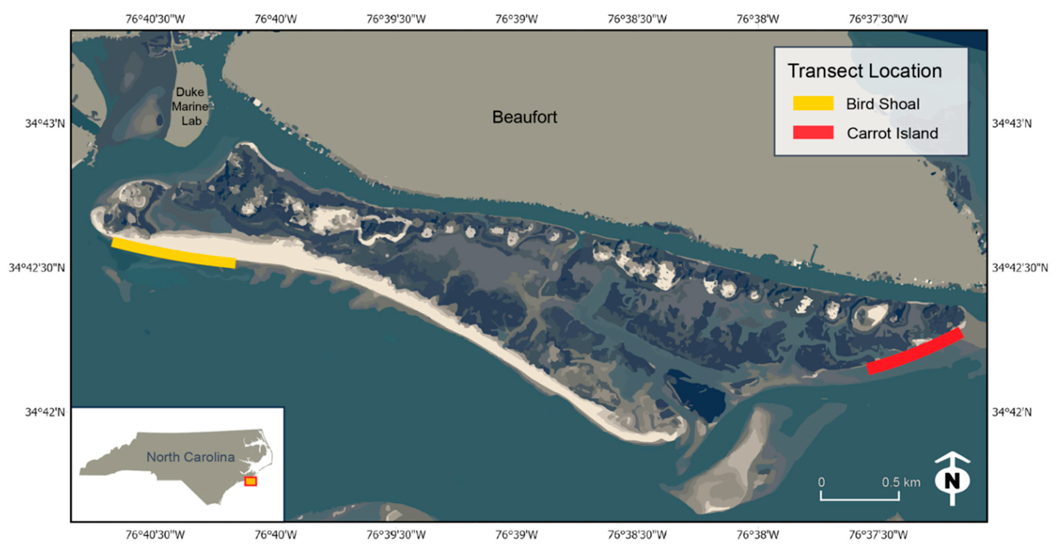
2.1. Study Area

Surveys of coastal sharks were conducted along the coastline (<10 m from shore) of the Rachel Carson Reserve (RCR) in Beaufort, North Carolina. The RCR is part of the North Carolina National Estuarine Reserve System, a network of ten protected sites along the North Carolina coast reserved for education, research, and stewardship managed by a federal-state partnership between the National Oceanic and Atmospheric Administration (NOAA) and the North Carolina Division of Coastal Management [32]. The RCR is comprised of four islands, covering over 2000 acres of area [32]. Bird Shoal and Carrot Island were selected as the two study sites, each representing different coastal habitats in the reserve (Figure 1). Bird Shoal represents sandy beach habitat, and Carrot Island represents both a salt marsh and oyster reef habitat. The close proximities of these sites to an inlet, which opens from the estuary to the open ocean, means that the sites were characterized by estuarine waters and impacted by inlet dynamics. However, the two sites were located at different distances to the inlet, so the intensity of inlet dynamics, including influxes of freshwater and the physical forces of tides, differed between the two sites. Surveys by UAS across each site covered approximately 1 km of coastline length.

2.2. UAS Imagery and Collection

Aerial surveys, resulting in video data, were conducted using a DJI Phantom 4 Quadcopter (n = 68) or DJI Mavic Pro Quadcopter (n = 9). Phantom quadcopters were equipped with a 1-inch 20-megapixel CMOS sensor and weighed approximately 3 lbs. Mavic Pro quadcopters were equipped with 12.35-megapixel sensors and weighed less than 2 lbs. Batteries used to power the UAS were lithium-ion polymer batteries. One battery was used per transect and allowed for 20–30 min of flight time flying at 3 m/s.
Flight paths were developed by manually flying the aircraft across a transect area using a flight controller. GPS waypoints (latitude, longitude) were dropped along the transect to develop a flight plan. Subsequent flights were flown over the same area, tracking the GPS points using the DJI Go 4 app, a flight-assistance application integrated with the DJI flight controller. Videos were collected by the 12.35-megapixel (Mavic Pro) or 20-megapixel (Phantom) aircraft camera at between 2720 × 1536–4096 × 2160 pixels, and a video speed of between 23–59 frames per second. Ground sampling distance was approximately 0.5–0.8cm per pixel depending on changes in UAS altitude and video resolution. Onboard SD cards recorded video information and were offloaded to computers during post-processing. UAS information (altitude, latitude, longitude) was recorded locally on the aircraft at a sampling rate of one observation per millisecond. Flight logs were downloaded during the post-processing phase.
Flights were conducted after sunrise and before sunset over the course of 17 days, from July 24th, 2019, to August 9th, 2019. A total of 77 UAS transects were conducted parallel to the shoreline. During each transect, approximately 1 km of coastline was covered (Figure 2). The camera field of view was approximately 30 m (perpendicular to the shoreline) by 15 m (parallel to the shoreline). Aircraft performance was sometimes limited by high winds and rain, preventing sampling during these times. Flights were conducted in compliance with the Federal Aviation Administration 14 CFR Part 107 regulations, and UAS operations were prevented in cases in which persons not involved in the UAS operation were occupying the study area. Aircrafts were launched and retrieved from a flat surface at the Duke Marine Lab for flights of Bird Shoal and ground-based launches were performed for flights of Carrot Island. Specialized launching equipment was not required. UAS details are provided in accordance with Barnas et al. 2020 [33].

2.3. Video Observation

Two independent reviewers identified individual sharks from each video transect, following observation methods of previous UAS-based studies of shark abundance [30,31]. Reviewers were trained to identify sharks by viewing example imagery and video clips. Videos were played at true speed in QuickTime Media Player. Videos were paused at each sighting to record the time stamp at which an individual entered the video frame to the nearest second. It was observed that the speed of the drone always outpaced the swimming speed of the sharks, so each sighted shark was assumed to be a new individual and double counts were not considered to impact the data. Discrepancies between the two individual counts were settled through a third review. For the third review, the lead author analyzed the transect video within a ten-second window around the reported time stamp of the sighting in question. Unlike the initial two observations, the third review allowed for replaying the video segment to reconcile the count discrepancy with greater certainty. An availability correction factor, used to correct for potential organisms present in the study area but not visible in the imagery [22], was not applied. Because all transects had maximum water depths <2 m, full detection was likely and environmental variables (e.g., water clarity, turbidity) were not assumed to impact shark availability for visual detection.

2.4. Environmental Data

Environmental data were collected from a NOAA buoy station at the Duke Marine Lab, proximate to both study sites (see Figure 1). For each transect, several variables were recorded (Table 2). Environmental variables were associated with each transect using time-date information. Original data is available in the Supplementary Information (S2, S3, S4).
Area covered by the transect varied slightly due to minor differences in transect strip length and flight altitude, which impacts strip width through field of view. In order to account for these differences in strip length and strip width of the transect, the area covered per transect was calculated. Strip length, defined as the distance traveled parallel to the coastline, was calculated from UAS log data. Strip width, defined as the field of view perpendicular to the coastline, was derived from the focal length of the UAS camera, flight altitude, and size of the sensor through Equation (1) from photogrammetry software Pix4D [34]:
S = (Sw × H)/F
where S is the strip width (m), Sw is UAS sensor width (mm), H is the height of the UAS flight (m), and F is the focal length of the UAS sensor (mm). Area covered by the UAS in a given transect was calculated by the Equation (2):
A = (S × 0.001) × (SL × 0.001)
where A represents transect area (km2), and S and SL are the length (m) and width (m) of the strip transect, respectively. Area is used to standardize abundance counts in correlation analyses and is included as an offset to abundance counts in the generalized linear model.

2.5. Statistical Analyses

2.5.1. Correlation Analyses

Correlation analyses were performed to assess relationships within environmental variables (predictors). Relatedness within predictors was explored to identify potential autocorrelation amongst environmental characteristics as well as the significance of date-driven trends. Because the transect observations were taken throughout time, date-driven trends (e.g., warming of air temperature from late July into early August) may have been represented in several variables selected for analyses. These relationships are explored through correlation plots and described by Pearson’s correlation coefficient (r) and significance (p, α = 0.05) for each variable pair. In the case of strongly correlated predictors, some variables were chosen for removal from further modeling.
Correlation analyses were also conducted to determine the strength of predictor relationships with observed shark density. For this section of the analysis, shark abundance counts were standardized over the transect area using Equations (1) and (2) (Section 2.4). To assess relationships with shark density (sharks/km2), Pearson’s correlation coefficient (r) and significance of the linear relationship (p, α = 0.05) were computed for numeric predictors, a Mann–Whitney U Test was performed for two-level categorical predictors Location and Time of Day, and a Kruskal–Wallis rank sum test was performed for four-level categorical variable tidal phase. While simple correlation analyses provided initial insights into the data, the dataset contains a large number of zero-count transects (n = 19) that may have obscured relationships using simple correlations. Moreover, simple correlations may miss logarithmic and other non-linear relationships between environmental variables and density. To further clarify these relationships, a generalized linear modeling structure was implemented.

2.5.2. Generalized Linear Model (GLM)

To parse apart the influence of individual variables on shark density, a generalized linear model (GLM) with a negative binomial error distribution and logarithmic link was constructed to estimate the relationship between the environmental conditions of each transect and the count of sharks observed. Several distributions were considered to explore changes in shark abundance. A Poisson distribution was examined, but a negative binomial distribution was ultimately chosen in order to accommodate potential overdispersion [35]. A zero-inflated negative binomial was tested to address apparent zero-inflation in the data, but was deemed unnecessary given that the incidence of structural zeroes, or zeros related to the ecological system rather than random zeros from sampling variability [36], was estimated to be small (<5%). Similarly, a “hurdle” model that combined a Bernoulli process with a truncated negative binomial was used to test zero deflation but did not demonstrate improvement over the ordinary negative binomial.
Traditionally, the negative binomial describes the process of drawing binary variables with success probability p until a given number of failures, r, occur. Substituting p = μ/(μ + Φ) and r = Φ allows us to reparameterize the distribution according to its mean μ, which is more useful for modeling purposes. The variance of this alternate paramaterization is equal to μ + μ2/Φ, so that Φ dictates the amount of overdispersion. The distribution converges toward a Poisson for large values of Φ. The model is described by Equations (3) and (4):
Y   ~   NegBin ( μ ,   ϕ )
log ( μ ) = X β + Ζ u + log ( A )
where we model μ using a mixed effects approach, with fixed coefficients Β for the environmental predictors and a random intercept u assigned to each sampling session (Equation (3)). We considered these random intercepts necessary to capture the dependence between consecutive flights during a single sampling session, when there was likely correlation between counts beyond what could be explained by the measured environmental factors. Here, Z is a design matrix assigning each observation to a session. All continuous predictors were normalized before fitting. The logarithm of the area surveyed (A) for each transect is included as an offset, since there was slight variation in the area covered in each transect.
We applied a Bayesian approach to estimate the parameters B, Φ, and Z. We chose wide, weakly informative priors for B (B ~ Normal (0, 10)) as well as Φ (Φ ~ Gamma (0.01, 0.01)). We drew the random effects (u) from a zero-centered normal distribution (u ~ Normal (0, σ2)), with a moderately informative hierarchical prior set on the variance (σ ~ Exponential (1)).
Best subset selection was performed across all possible subsets of the seven predictors. Models were evaluated and compared using leave-one-group-out cross validation (LOGO-CV). This approach is similar to K-fold cross-validation [37], but observations were grouped to sampling sessions (consisting of 1–4 transects in sequence) and each session was held out from the fitting process and then predicted on. The evaluation criterion was the estimated log predictive density (ELPD) accumulated across the out-of-sample points. While the goal of the study is not to maximize predictiveness, using out-of-sample predictive power is an effective way to simplify our model and avoid spurious relationships.
In many cases, the computation required for both best subset selection and “brute-force” ELPD estimates (as opposed to an approximation) is prohibitively expensive. It was feasible, however, for our dataset of 77 transects with 29 unique sampling sessions. The model was fit using the RStan package in R (v.4.0.2) [38,39]. Given a hierarchical model structure, the Stan language implements the Hamiltonian Monte Carlo algorithm to draw samples from a target distribution [38]. The script used for model generation is available in the Supplementary Information (S5, S6). For each model in consideration, we ran four chains initialized with random values from the prior distributions. Each chain ran for 2000 iterations, 1000 of which were used for warm-up. Based on the potential scale reduction statistic ( R ^ ), there was no evidence of non-convergence.

3. Results

A total of 381 sharks were sighted over the course of 77 transects. Observer counts of sharks had high levels of agreement (difference = 0.60 ± 0.66 individuals) and demonstrated identical sightings in 53 transects. A third review reconciled count differences of one (n = 21) or two (n = 3) sharks, the majority of which confirmed the presence of an individual missed by one observer (82% of count discrepancies). The resultant median density across all transects was 74.8 sharks/km2 (median = 74.8, IQR = (13.9, 298)). The distribution of shark density was right skewed, impacted by zero-shark transects (n = 19). The original dataset used for analysis is available in Supplementary Information (S1).

3.1. Species Identification

This study examined coastal shark dynamics at large as opposed to a targeted species-specific population analysis. Due to limits of the UAS imagery resolution and sparse literature on the aerial identification of sharks, this UAS-based methodology did not allow for positive species identification. However, several shark species matching the body size and shape observed from the UAS that are known to frequent the area were blacktip, blacknose, Atlantic sharpnose, spiny dogfish, smooth dogfish, bonnethead, bull, and sandbar sharks [40]. Several of these species, though, were unlikely to be represented in the survey: bull sharks are thought to prefer estuaries near river mouths [8]. Spiny dogfish and Sandbar sharks have been shown to be rare in nearby estuaries during the summer months [8], and Bonnethead sharks observed in exploratory UAS studies prior to the sampling transects showed a distinctive spade-like head that was not observed during the sampling session. Several Blacktip sharks were observed during the sampling transects, identifiable by dark black tips on the pectoral and dorsal fins, but the majority of sharks in this study lacked this feature. For these reasons, it was likely that the majority of sharks observed in this study were Atlantic Sharpnose, Smooth Dogfish, or Blacknose sharks.

3.2. Correlation Analyses

Bivariate combinations of environmental variables were plotted and analyzed to understand relationships between predictors of shark density (Figure 3). Six of the 15 continuous variable pairs were significantly correlated (p < 0.05) with each other. The variables water temperature, pressure, and wind speed demonstrated highly significant correlations with day elapsed (r = 0.75, −0.65, −0.45 (respectively), p < 0.001). To avoid highly correlated predictors variables, day elapsed was dropped from statistical modeling. Also, the distribution of samples across tidal phase categories demonstrates an uneven number of samples across tidal phase categories (Tidal Phase x Tidal Phase matrix cell, Figure 3). With more samples during ebb tides (n = 48) than flood, high, and low tides combined (n = 29), tidal phase was dropped from the modeling analysis.
Before model construction, individual relationships between environmental variables and shark density were assessed (Figure 4). Wind speed (p < 0.05), pressure (p < 0.01), water temperature (p < 0.01), time relative to dawn/dusk (p < 0.01), day count (p < 0.001), and location (p < 0.001) all demonstrated significant relationships with shark density. Wind speed and pressure showed negative relationships with density while water temperature and day count appeared to be positively correlated with density. Within each session (a series of 1–4 transects performed after sunrise or before sunset on a given day), time relative to dawn/dusk demonstrated a negative relationship with proportional density. In other words, transects closer to dawn and dusk (less time elapsed from sunrise/sunset) were associated with the greatest shark density while transects farther from dawn and dusk were associated with progressively lower shark densities, comparatively. Analyzing the categorical variables, it can be seen that significantly greater shark density was observed at Bird Shoal relative to Carrot Island (Mann–Whitney U test). The variables considered for predictive analysis using a GLM were wind speed, pressure, water temperature, tidal height, time relative to dawn/dusk, location, and time of day.

3.3. Model

While all subsets of the chosen environmental predictors were considered for the GLM, out-of-sample predictive accuracy, as measured by expected log predictive density (ELPD), was maximized when using the following four variables to predict count: wind speed, water temperature, time relative to dawn and dusk, and location. In addition to the highest ELPD, our final model had a root mean square error (RMSE) of 4.38 and a median absolute error (MAE) of 2.13 for out-of-sample observations using predicted counts based on the posterior means of all the estimated parameters (Figure 5).
The model was most confident in the direction of the parameters for time relative to dawn/dusk and location, as the entire 95% credible intervals for both of those coefficients were below zero (Figure 6). The direction of the effect of wind speed and water temperature were not as unambiguous, but their 80% and 50% credible intervals, respectively, also did not include zero.
As a result of the logarithmic link between the linear predictor and the expected value of the negative binomial, the effect of parameters on the count is non-linear (Table 3). However, using an example of eight sharks (median of n = 44 counts at Birds Shoal), the final model implies the following associations: (1) Wind Speed: An increase of 1 m/s in windspeed would decrease the expected shark count to 6.82, (2) Water Temperature: An increase of 1° in water temperature would increase the expected shark count to 9.32, (3) Time Relative to Dawn/Dusk: An additional 10 min after dawn (or before dusk) would decrease the expected shark count to 6.96, and (4) Location: Moving locations to Carrot Island would decrease the expected shark count to 0.62.
These effect sizes are moderate, implying that much of the variation in shark abundance cannot be explained by the covariates alone. As a result, the scale of the random intercepts is relatively large. The standard deviation of random intercepts (σ) was estimated to be 0.69 (95% CI: 0.42–1.04), with a range in the posterior means of −0.73 to 0.95. To illustrate the impact of these parameters, consider session 12, which had an estimated random intercept of 0.48, the 14th largest of all 29 intercepts in terms of absolute value. The in-sample predicted counts for the two transects from session 12 were 8.96 and 10.98, compared to the actual counts of 12 and 9, respectively. Without the boost from the random intercept, those predicted counts would be 5.56 and 6.81.
The ability of these parameters to account for some of the remaining variance in the counts allowed for large values of Φ (posterior mean of 79.02, 95% CI: 11.64–264.01) in the posterior, indicating only limited levels of overdispersion and implying that Poisson regression would likely also be an adequate choice in this study. However, even large values of Φ can only diminish overdispersion so much for high counts (i.e., 20 sharks or more), and we think the added flexibility of the negative binomial makes it a wise choice for future research. Moreover, without the use of a random effect to explain some of the variability, Φ would be much lower.

4. Discussion

The results of the present study indicate that the density of sharks is driven by a combination of fine-scale physical forcing elements in the local coastal ecosystem at the RCR. These relationships are discussed in detail below. These results also indicate that UAS can be used effectively in temperate estuaries to study the distribution and density of estuarine sharks, representing a cost effective and non-invasive approach available to researchers.
Weather—Water temperature was found to be positively correlated with shark density (r = 0.32, p < 0.01, Figure 4). This is supported by the GLM parameters, which predicts that, at an abundance of 8 sharks, a 1° increase in water temperature would increase the predicted count by 1.32 individuals. This supports the original hypothesis that more sharks would be observed in warmer waters (Table 1) given that, on an annual scale, more sharks are observed in these areas in summer months and associated warmer waters [41]. Also, other studies investigating the impact of long-term temperature trends on similar species in coastal estuarine landscapes support this positive relationship [8,12,13,14]. Warmer waters may be used for thermoregulation as a result of physiological constraints or in response to the temperature ranges and associated distribution of prey in these ecosystems. However, this relationship may be driven partially by the linear increase in water temperature over the sampling session, shown by the strong correlation between water temperature and day count (r = 0.75, p < 0.001, Figure 3). Because temperature is associated with seasonality, and with higher temperatures in summer months and cooler temperatures in winter months, this may indicate that shark abundance is seasonally influenced. Though this has been recognized on a large scale [42], this result may provide increased resolution of small-scale variability in abundance on the scale of weeks, not just seasonally over the course of a year. Because this study did not capture peak water temperatures, the peak of shark abundance in these estuaries may be even higher than observed from transects in early August. Though this study indicates that shark abundance increases linearly over time from late July into early August (time series (day): r = 0.50, p < 0.001), future studies should investigate the possibility that shark abundance in the estuaries’ peaks in late August or even early September.
Wind speed was significantly negatively correlated with shark density, and at high wind speeds, lower shark density was observed (r = −0.27, p < 0.05, Figure 4). This significant negative correlation with shark abundance indicates that wind speed may impact shark presence in the estuary. This relationship is supported by the GLM results, which predict that with an abundance of 8 sharks in a given transect, a 1 m/s increase in wind speed would decrease the expected count by 1.18 individuals. This supports the original prediction that, in high winds, fewer sharks would be present (Table 1) as winds impact shallow water environments through the generation of surface currents [43]. These surface currents may present increased difficulty of locomotion through the estuary with the risk of stranding. However, it should be noted that UAS were not operational at high wind speeds (>6 m/s), and so this trend is not representative of the full range of wind speed values at the study sites. An additional potential drawback to using a UAS-based methodology is that wind speed has been cited as a factor impacting shark detection probability by UAS in temperate estuaries [44]. However, the conditions of this study make it highly unlikely that environmental variation would lead to changes in detection. In contrast to Benavides et al. (2020), which tested the abilities of UAS to detect bonnethead sharks in temperate estuaries, this study used video data, rather than still images, to detect moving objects, which added to their visibility. Moreover, transects were flown at a lower altitude than Benavides et al. (2020), resulting in an increased resolution at ground sampling distance (GSD) of 0.5–0.8 cm/pixel compared to the GSD of ~2 cm/pixel used by Benavides et al. (2020). The results of lower shark abundance in the estuary at high wind speeds may be due to avoidance of strong surface currents that might limit mobility within the estuary. For this reason, it is possible that sharks use deeper water environments that are less impacted by wind-induced surface currents when wind speeds are high. An extension of this study would be to analyze the magnitude and direction of surface currents as well as other estuarine currents in association with shark abundance.
Pressure was significantly correlated with shark density (r = −0.34, p < 0.01, Figure 5), but was not selected as a strong predictor of abundance in the GLM. Fewer sharks were anticipated in the estuary at low barometric pressure because decreases in barometric pressure, associated with storms, have been linked to shark movement out of estuarine habitats. However, these movements may be species-specific and the magnitude of pressure change required to induce movement has not been well quantified [42]. While barometric pressure has been shown to influence shark movement, studies that support these conclusions are widely focused on severe changes in pressure (e.g., before a hurricane) [42,45]. The significant correlation of pressure and shark density may provide evidence that elasmobranchs respond to fine-scale changes in pressure, although the significant correlation of pressure with water temperature may be driving the individual relationship and explain the absence of pressure in GLM variable selection (Figure 3).
Tides—Tidal height was not significantly correlated with shark density in the correlation analyses (p > 0.05, Figure 4). After GLM variable selection, tidal height was dropped from the final model. It was expected that increased density might be observed with higher tides (Table 1) based on physical forcing into the estuary and increased relative water depth. Though shark movement in response to tides has been shown to vary [8], a study of juvenile sandbar sharks in the southeastern United States demonstrated movement in the direction of tidal flow [8]. The data do not support this hypothesis. However, although tidal phase (pointing to tidal direction) was excluded from this analysis given that some phases were sparsely represented, future research should target varied tidal stages to understand the impact of tidal direction on shark movement. This would provide greater insights into estuarine habitat utilization given that movement of sharks in the direction of tides in similar nearshore environments of the southeastern United States coast has been cited in previous studies.
Time—Within sampling sessions (repeated samples following dawn or preceding dusk), time relative to dawn and dusk was significantly correlated with proportional shark density. There appeared to be a trend of decreasing activity moving into the day with higher observed density close to sunrise and sunset (Figure 4). This is supported by the results of the GLM, which indicate that, at an abundance of 8 sharks, increasing time by 10 min after dawn (or before dusk) would decrease the expected shark count by 1.04 individuals. This supports the initial expectation that shark density would decrease with time elapsed from dawn or dusk due to the crepuscular activity of many elasmobranchs [42]. This is similar to other studies that indicate elasmobranchs exhibit crepuscular behavior, with more activity closer to sunrise and sunset [42,46,47]. In order to understand the influence of time relative to sunrise and sunset on shark abundance, additional transects should be done within a given sampling session.
Between dawn and dusk transects, there appeared to be no significant difference in density (Mann–Whitney U Test, p > 0.05), supporting the prediction of no relationship between dawn and dusk sampling sessions (Table 1). Sharks were expected to be similarly observed between dawn and dusk sessions as crepuscular behavior indicates increasing activity near both sunrise and sunset, but does not distinguish between them.
Although day of the study period was found to be significantly positively correlated with density (Figure 4), it was strongly correlated with environmental variable water temperature (Figure 3) and dropped from further analysis in the GLM. In contrast to the results, day of the study period (day count) was anticipated to be negatively correlated with abundance given that sharks in this area are thought to reach peak abundance in July, before or near the beginning of the study period. A study of shark activity in Pamlico Sound, an estuarine area slightly north of the study site in the present study, shows that common shark species in this area appear to peak in abundance in July and move out of the estuary in greater numbers in August [8]. It is possible that the correlation of day count with several other variables in the analysis (Figure 3) may have obscured our ability to isolate the true trend of density throughout time (on the scale of days).
Location—The significant difference between shark abundance at the two study sites (Figure 4, Mann–Whitney U Test, p < 0.001) indicates that shark abundance may be impacted by site characteristics. This is supported by the GLM, which predicts that at a transect abundance of 8 sharks, changing locations from Bird Shoal to Carrot Island would decrease the expected abundance by 7.38 individuals. These data support the original hypothesis that higher shark density would be observed at Bird Shoal (Table 1). The direction and high magnitude of site location’s influence on abundance may be attributed to several factors. One important difference between locations is the distance of each site to the inlet, which opens to the ocean. Bird Shoal, which was characterized by significantly higher shark abundance, is located closer to the inlet (approx. 1.5 km, straight-line distance) whereas Carrot Island is located farther away (approx. 4 km) (Figure 1). Given previous studies investigating the impact of inlet proximity on shark abundance [8,33], higher density was expected at the sampling site closer to the inlet as areas with access to open water may be preferred for organisms navigating between open water and estuarine habitats. The idea that abundance may vary based on distance to an inlet is supported by several other studies of coastal sharks found in these nearshore estuarine environments. A study in the Pamlico sound, a similar estuarine area slightly north of the study sites in this analysis, found that shark presence was strongly associated with distance to an inlet and that inlet distance may be one of the main drivers of these sharks’ presence in these areas [8]. Other studies supporting this conclusion include an analysis of estuaries in the Florida panhandle where there was increased shark abundance at inlets to the Gulf of Mexico [13] and Texas estuaries where sharks were observed almost exclusively near inlets [14]. The result of this study, along with the results from these previous studies, indicate that sharks may select estuarine areas near inlets to have better access to open water.
There are other characteristics of the study sites that may also be driving shark abundance differences between Bird Shoal and Carrot Island. Bird Shoal has a mostly sandy beach habitat, whereas Carrot Island is mostly oyster reef and salt marsh habitat. However, inlet proximity is also linked to salinity, with salinity tending to decrease with greater distance from the inlet [8]. Given salinity gradients observed at a similar site [8], it is possible that the two study sites differ in salinity, with the site closer to open water (Bird Shoal) having higher saline content and the site farther from open ocean (Carrot Island) having lower saline content. One limitation of this study is that these site-specific attributes cannot be decoupled. For future studies, the addition of study sites at varying distances from the inlet but with similar coastal habitats would allow for a greater understanding of the impact of inlet distance while controlling for habitat type. Alternatively, having more study sites across a range of coastal habitats with similar distances to the inlet would be helpful for parsing out habitat type preferences. Using this demonstrated drone methodology could allow for rapid, broader surveying of these coastal habitats with limited disturbance to the study species. Furthermore, future studies could be enhanced by employing new video-based machine learning techniques to identify sharks as opposed to manual counts [48]. With a clear species identification, biological inferences about habitat preference and salinity ranges could be made in response to these types of studies. To address the species identification limitations of this study, a combined methodology is proposed for future work synthesizing high-resolution sub-surface data, such as baited remote underwater videos (BRUVs) known to successfully observe sharks [49], and aerial data to identify individual species while also observing population-wide dynamics.

5. Conclusions

This study provides new information about shark density dynamics within the RCR, an area frequented by tourists and locals for recreation. This study suggests that coastal shark density in the temperate estuarine landscapes of Beaufort, NC, may increase at times closer to dawn and dusk and in locations potentially closer to an open ocean inlet as well as conditions of warm water temperatures and low wind speeds. Future studies should explore the predictive capacity of these variables to understand shark activity in other estuaries across a wide range of conditions. These analyses lay the groundwork for future studies assessing shark abundance responses to fine-scale variation in abiotic conditions and provide a novel methodological framework using UAS to assess shark abundance in coastal estuaries.

Supplementary Materials

Supplementary Materials are available online at https://www.mdpi.com/2504-446X/4/4/74/s1. Scripts and original data are available in the supplementary files.

Author Contributions

Conceptualization, A.E.D.; methodology, A.E.D. and J.T.R.; formal analysis, A.E.D. and W.E.H.; investigation, A.E.D.; resources, D.W.J.; data curation, A.E.D.; writing—original draft preparation, A.E.D. and W.E.H.; writing—review and editing, J.T.R. and D.W.J.; visualization, A.E.D. and W.E.H.; supervision, J.T.R. and D.W.J.; project administration, A.E.D. and D.W.J.; funding acquisition, A.E.D. and D.W.J. All authors have read and agreed to the published version of the manuscript.

Funding

This research was supported by Duke University Bass Connections and the Duke University Rachel Carson Scholars Program.

Acknowledgments

The authors wish to acknowledge support from the Marine Robotics and Remote Sensing Laboratory (MaRRS Lab) and the Duke Marine Laboratory (DUML) at Duke University. We would like to specifically thank Julian Dale and Everett Newton of the MaRRS Lab for UAS flight training and execution support. The authors wish to thank Meagan Dunphy-Daly of Duke University for funding assistance through the Duke University Rachel Carson Scholars Program and scientific mentorship of the lead author. We appreciate the field support from students of DUML’s Summer 2019 Drones in Marine Science and Conservation course. We would also like to thank independent observers Alicia Porile, Ally Livingston, Emily Fechner, Emma Schmaltz, Julia Saveliff, Madeleine Cochrane, and Sakiko Nishida of Duke University for volunteering their time to support this research.

Conflicts of Interest

The authors declare no conflict of interest.

References

  1. Noss, R.F.; Platt, W.J.; Sorrie, B.A.; Weakley, A.S.; Means, D.B.; Costanza, J.; Peet, R.K. How global biodiversity hotspots may go unrecognized: Lessons from the North American Coastal Plain. Divers. Distrib. 2015, 21, 236–244. [Google Scholar] [CrossRef]
  2. Barbier, E.B.; Hacker, S.D.; Kennedy, C.; Koch, E.W.; Stier, A.C.; Silliman, B.R. The value of estuarine and coastal ecosystem services. Ecol. Monogr. 2011, 81, 169–193. [Google Scholar] [CrossRef]
  3. Mehvar, S.; Filatova, T.; Dastgheib, A.; de Ruyter van Steveninck, E.; Ranasinghe, R. Quantifying economic value of coastal ecosystem services: A review. J. Mar. Sci. Eng. 2018, 6, 5. [Google Scholar] [CrossRef] [Green Version]
  4. Suchanek, T.H. Temperate coastal marine communities: Biodiversity and threats. Integr. Comp. Biol. 1994, 34, 100–114. [Google Scholar] [CrossRef]
  5. Knip, D.M.; Heupel, M.R.; Simpfendorfer, C.A. Sharks in nearshore environments: Models, importance, and consequences. Mar. Ecol. Prog. Ser. 2010, 402, 1–11. [Google Scholar] [CrossRef]
  6. Moxley, J.; Skomal, G.; Chisholm, J.; Halpin, P.; Johnston, D. Daily and seasonal movements of Cape Cod gray seals vary with predation risk. Mar. Ecol. Prog. Ser. 2020, 644, 215–228. [Google Scholar] [CrossRef]
  7. Dill, L.M.; Heithaus, M.R.; Walters, C.J. Behaviorally mediated indirect interactions in marine communities and their conservation implications. Ecology 2003, 84, 1151–1157. [Google Scholar] [CrossRef] [Green Version]
  8. Bangley, C.W.; Paramore, L.; Dedman, S.; Rulifson, R.A. Delineation and mapping of coastal shark habitat within a shallow lagoonal estuary. PLoS ONE 2018, 13, e0195221. [Google Scholar] [CrossRef]
  9. Haulsee, D.E.; Breece, M.W.; Miller, D.C.; Wetherbee, B.M.; Fox, D.A.; Oliver, M.J. Habitat selection of a coastal shark species estimated from an autonomous underwater vehicle. Mar. Ecol. Prog. Ser. 2015, 528, 277–288. [Google Scholar] [CrossRef] [Green Version]
  10. Dean Grubbs, R.; Musick, J.A. Spatial Delineation of Summer Nursery Areas for Juvenile Sandbar Sharks in Chesapeake Bay, Virginia. In Shark Nursery Grounds of the Gulf of Mexico and the East Coast Waters of the United States; American Fisheries Society: New York, NY, USA, 2007; Volume 50, pp. 63–86. Available online: https://fisheries.org/bookstore/all-titles/afs-symposia/54053p/ (accessed on 10 November 2020).
  11. Sagarese, S.R.; Frisk, M.G.; Cerrato, R.M.; Sosebee, K.A.; Musick, J.A.; Rago, P.J. Application of generalized additive models to examine ontogenetic and seasonal distributions of spiny dogfish (Squalus acanthias) in the Northeast (US) shelf large marine ecosystem. Can. J. Fish. Aquat. Sci. 2014, 71, 847–877. [Google Scholar] [CrossRef]
  12. Simpfendorfer, C.A.; Freitas, G.G.; Wiley, T.R.; Heupel, M.R. Distribution and habitat partitioning of immature bull sharks (Carcharhinus leucas) in a southwest Florida estuary. Estuaries 2005, 28, 78–85. [Google Scholar] [CrossRef]
  13. Ward-Paige, C.A.; Britten, G.L.; Bethea, D.M.; Carlson, J.K. Characterizing and predicting essential habitat features for juvenile coastal sharks. Mar. Ecol. 2015, 36, 419–431. [Google Scholar] [CrossRef]
  14. Froeschke, J.; Stunz, G.W.; Wildhaber, M.L. Environmental influences on the occurrence of coastal sharks in estuarine waters. Mar. Ecol. Prog. Ser. 2010, 407, 279–292. [Google Scholar] [CrossRef]
  15. Ellis, J.R.; McCully Phillips, S.R.; Poisson, F. A review of capture and post-release mortality of elasmobranchs. J. Fish Biol. 2017, 90, 653–722. [Google Scholar] [CrossRef] [PubMed]
  16. Hueter, R.E.; Manire, C.A.; Tyminski, J.P.; Hoenig, J.M.; Hepworth, D.A. Assessing Mortality of Released or Discarded Fish Using a Logistic Model of Relative Survival Derived from Tagging Data. Trans. Am. Fish. Soc. 2006, 135, 500–508. [Google Scholar] [CrossRef] [Green Version]
  17. Rulifson, R.A. Spiny Dogfish Mortality Induced by Gill-Net and Trawl Capture and Tag and Release. N. Am. J. Fish. Manag. 2007, 27, 279–285. [Google Scholar] [CrossRef]
  18. Huish, M.T.; Benedict, C. Sonic Tracking of Dusky Sharks in the Cape Fear River, North Carolina. J. Elisha Mitchell Scien. Soc. 1978, 93, 21–26. [Google Scholar]
  19. Hammerschlag, N.; Gallagher, A.J.; Lazarre, D.M. A review of shark satellite tagging studies. J. Exp. Mar. Biol. Ecol. 2011, 398, 1–8. [Google Scholar] [CrossRef]
  20. Jewell, O.J.D.; Wcisel, M.A.; Gennari, E.; Towner, A.V.; Bester, M.N.; Johnson, R.L.; Singh, S. Effects of smart position only (SPOT) tag deployment on white sharks carcharodon carcharias in South Africa. PLoS ONE 2011, 6, e27242. [Google Scholar] [CrossRef] [Green Version]
  21. Rowat, D.; Gore, M.; Meekan, M.G.; Lawler, I.R.; Bradshaw, C.J.A. Aerial survey as a tool to estimate whale shark abundance trends. J. Exp. Mar. Biol. Ecol. 2009, 368, 1–8. [Google Scholar] [CrossRef]
  22. Kessel, S.T.; Gruber, S.H.; Gledhill, K.S.; Bond, M.E.; Perkins, R.G. Aerial Survey as a Tool to Estimate Abundance and Describe Distribution of a Carcharhinid Species, the Lemon Shark, Negaprion brevirostris. J. Mar. Biol. 2013, 2013, 597383. [Google Scholar] [CrossRef] [Green Version]
  23. Acuña-Marrero, D.; Smith, A.; Salinas-de-León, P.; Harvey, E.; Pawley, M.; Anderson, M. Spatial patterns of distribution and relative abundance of coastal shark species in the Galapagos Marine Reserve. Mar. Ecol. Prog. Ser. 2018, 593, 73–95. [Google Scholar] [CrossRef]
  24. Osgood, G.J.; McCord, M.E.; Baum, J.K. Using baited remote underwater videos (BRUVs) to characterize chondrichthyan communities in a global biodiversity hotspot. PLoS ONE 2019, 14, e0225859. [Google Scholar] [CrossRef] [PubMed]
  25. White, J.; Simpfendorfer, C.A.; Tobin, A.J.; Heupel, M.R. Application of baited remote underwater video surveys to quantify spatial distribution of elasmobranchs at an ecosystem scale. J. Exp. Mar. Biol. Ecol. 2013, 448, 281–288. [Google Scholar] [CrossRef]
  26. Johnston, D.W. Unoccupied aircraft systems in marine science and conservation. Annu. Rev. Mar. Sci. 2019, 11, 439–463. [Google Scholar] [CrossRef] [PubMed] [Green Version]
  27. Koski, W.R.; Allen, T.; Ireland, D.; Buck, G.; Smith, P.R.; Macrender, A.M.; Halick, M.A.; Rushing, C.; Sliwa, D.J.; McDonald, T.L. Evaluation of an unmanned airborne system for monitoring marine mammals. Aquat. Mamm. 2009, 35, 347–357. [Google Scholar] [CrossRef]
  28. Loughlin, T.R.; Perlov, A.S.; Vladimirov, V.A. Range-wide survey and estimation of total number of steller sea lions in 1989. Mar. Mammal Sci. 1992, 8, 220–239. [Google Scholar] [CrossRef]
  29. Marsh, H.; Sinclair, D.F. An experimental evaluation of dugong and sea turtle aerial survey techniques. Wildl. Res. 1989, 16, 639–650. [Google Scholar] [CrossRef]
  30. Hensel, E.; Wenclawski, S.; Layman, C.A. Using a small, consumer-grade drone to identify and count marine megafauna in shallow habitats. Lat. Am. J. Aquat. Res. 2018, 46, 1025–1033. [Google Scholar] [CrossRef]
  31. Kiszka, J.; Mourier, J.; Gastrich, K.; Heithaus, M. Using unmanned aerial vehicles (UAVs) to investigate shark and ray densities in a shallow coral lagoon. Mar. Ecol. Prog. Ser. 2016, 560, 237–242. [Google Scholar] [CrossRef]
  32. NC DEQ: Rachel Carson Reserve. Available online: https://deq.nc.gov/about/divisions/coastal-management/nc-coastal-reserve/reserve-sites/rachel-carson-reserve (accessed on 10 November 2020).
  33. Barnas, A.F.; Chabot, D.; Hodgson, A.J.; Johnston, D.W.; Bird, D.M.; Ellis-Felege, S.N. A standardized protocol for reporting methods when using drones for wildlife research. J. Unmanned Veh. Syst. 2020, 8, 89–98. [Google Scholar] [CrossRef] [Green Version]
  34. TOOLS—GSD Calculator—Support. Available online: https://support.pix4d.com/hc/en-us/articles/202560249-TOOLS-GSD-calculator (accessed on 10 November 2020).
  35. Lindén, A.; Mäntyniemi, S. Using the negative binomial distribution to model overdispersion in ecological count data. Ecology 2011, 92, 1414–1421. [Google Scholar] [CrossRef] [PubMed]
  36. Blasco-Moreno, A.; Pérez-Casany, M.; Puig, P.; Morante, M.; Castells, E. What does a zero mean? Understanding false, random and structural zeros in ecology. Methods Ecol. Evol. 2019, 10, 949–959. [Google Scholar] [CrossRef]
  37. Gelman, A.; Carlin, J.B.; Stern, H.S.; Dunson, D.B.; Vehtari, A.; Rubin, D.B.; Carlin, J.; Stern, H.; Rubin, D.; Dunson, D. Bayesian Data Analysis, 3rd ed.; CRC Press: Boca Raton, FL, USA, 2013. [Google Scholar]
  38. Stan Development Team. “RStan: The R Interface to Stan.” R Package Version 2.21.2. 2020. Available online: http://mc-stan.org/ (accessed on 10 November 2020).
  39. RStudio Team. RStudio: Integrated Development for R. RStudio, PBC, Boston, MA. 2020. Available online: http://www.rstudio.com/ (accessed on 10 November 2020).
  40. Pamlico Sound Independent Gill Net Survey [2009: July 1–2014: June 30]—State Publications II—North Carolina Digital Collections. Available online: https://digital.ncdcr.gov/digital/collection/p16062coll9/id/170689/rec/7 (accessed on 10 November 2020).
  41. Schwartz, F.J. Occurrence, Abundance, and Biology of the Blacknose Shark, Carcharhinus acronotus, in North Carolina. Northeast Gulf Sci. 1984, 7, 29–47. [Google Scholar] [CrossRef] [Green Version]
  42. Schlaff, A.M.; Heupel, M.R.; Simpfendorfer, C.A. Influence of environmental factors on shark and ray movement, behaviour and habitat use: A review. Rev. Fish Biol. Fish. 2014, 24, 1089–1103. [Google Scholar] [CrossRef]
  43. Elliott, A.; Aj, E. Wind-Driven Flow in a Shallow Estuary. Oceanologica Acta 1982, 5, 7–10. [Google Scholar]
  44. Benavides, M.T.; Fodrie, F.J.; Johnston, D.W. Shark detection probability from aerial drone surveys within a temperate estuary. J. Unmanned Veh. Syst. 2020, 8, 44–56. [Google Scholar] [CrossRef]
  45. Heupel, M.R.; Simpfendorfer, C.A.; Hueter, R.E. Running before the storm: Blacktip sharks respond to falling barometric pressure associated with Tropical Storm Gabrielle. J. Fish Biol. 2003, 63, 1357–1363. [Google Scholar] [CrossRef]
  46. Andrews, K.S.; Williams, G.D.; Farrer, D.; Tolimieri, N.; Harvey, C.J.; Bargmann, G.; Levin, P.S. Diel activity patterns of sixgill sharks, Hexanchus griseus: The ups and downs of an apex predator. Anim. Behav. 2009, 78, 525–536. [Google Scholar] [CrossRef]
  47. Nelson, D.R.; McKibben, J.N.; Strong, W.R.; Lowe, C.G.; Sisneros, J.A.; Schroeder, D.M.; Lavenberg, R.J. An acoustic tracking of a megamouth shark, Megachasma pelagios: A crepuscular vertical migrator. Environ. Biol. Fishes 1997, 49, 389–399. [Google Scholar] [CrossRef]
  48. Gorkin, R.; Adams, K.; Berryman, M.J.; Aubin, S.; Li, W.; Davis, A.R.; Barthelemy, J. Sharkeye: Real-Time Autonomous Personal Shark Alerting via Aerial Surveillance. Drones 2020, 4, 18. [Google Scholar] [CrossRef]
  49. Brooks, E.; Sloman, K.; Sims, D.; Danylchuk, A. Validating the use of baited remote underwater video surveys for assessing the diversity, distribution and abundance of sharks in the Bahamas. Endanger. Species Res. 2011, 13, 231–243. [Google Scholar] [CrossRef]
Figure 1. Field sites at the Rachel Carson Reserve (RCR) in Beaufort, North Carolina, represent different coastal habitats and distances to an inlet to open water. Bird shoal is characterized by sandy beach habitat and a closer proximity to the inlet, while Carrot Island consists of salt marsh and oyster reef habitat and is located farther from the inlet.
Drones 04 00074 g001
Figure 2. Field operations using Unoccupied Aircraft Systems (UAS) to observe coastal shark density along transects parallel to shore. (A) Study design schematic. (B) True example video frame at Bird Shoal (enlarged for visualization purposes).
Drones 04 00074 g002
Figure 3. Correlation matrix of environmental variables demonstrates significant correlations between several variable pairs. Pearson’s correlation coefficient was used to assess relationships. *: p < 0.05, ***: p < 0.001.
Drones 04 00074 g003
Figure 4. Relationships of environmental variables with shark density. Environmental data were derived from a local buoy (Table 2) and variables were correlated with standardized shark density (sharks/km2) or, for time relative to dawn/dusk, proportional density (proportion of sharks observed of total observed during that sampling session). Correlations were calculated using Pearson’s correlation coefficient for continuous variables, an independent Mann–Whitney U test for two-level categorical variables (Location, Time of Day), and a Kruskal–Wallis rank sum test for four-level categorical variables (Tidal Phase). *: p < 0.05, **: p < 0.01, ***: p < 0.001.
Drones 04 00074 g004
Figure 5. Predicted shark abundance demonstrates close agreement with actual (true) shark abundance. Out-of-sample predicted abundance counts were generated using the posterior means of all estimated parameters in the final Generalized Linear Model (GLM).
Drones 04 00074 g005
Figure 6. Posterior distributions of the five fixed effects. Demarcations represent the mean and boundaries of a 95% credible interval.
Drones 04 00074 g006
Table 1. Hypothesized impact of environmental conditions on shark density. For continuous variables, expected relationship direction is shown (+: positive relationship predicted, −: negative relationship predicted, NA: no relationship predicted). For categorical variables, the relative density across levels is predicted (e.g., greater density is expected to be associated with high tides than low tides). Expected relationships are postulated based on previous research and biological and physiological knowledge of coastal shark species.
VariableExpected Relationship with Shark Density
Tidal Height+
Tidal PhaseHigh: +, Ebb: −, Low: −, Flood: +
Water Temperature+
Wind Speed
Barometric Pressure+
Time of DayDawn: NA, Dusk: NA
Time (minutes elapsed from dawn/dusk)
Day Count
LocationBird Shoal: +, Carrot Island: −
Table 2. Environmental variables used to understand changes in shark density. Associated data sources, sampling intervals, and details are provided. NOAA: National Oceanic and Atmospheric Administration. NA: Not applicable.
VariableSourceRecording IntervalData Details
Tidal Height (m)NOAA Tide & Currents, Tides/Water Levels
Station ID: 8656483, Duke Marine Lab, Beaufort, NC
6 minWater level relative to Mean Lower Low Water (MLLW)
Tidal PhaseNOAA Tide & Currents, Tides/Water Levels
Station ID: 8656483, Duke Marine Lab, Beaufort, NC
1 minDefined as:
High: within ± 1 h of reported high tide
Low: within ± 1 h of reported low tide
Ebb: Water level decreasing, from high to low tide
Flood: Water level increasing, from low to high tide
Water temperature (°C)NOAA Tide & Currents, Meteorological Observations
Station ID: 8656483, Duke Marine Lab, Beaufort, NC
6 min
Wind speed (m/s)NOAA Tide & Currents, Meteorological Observations
Station ID: 8656483, Duke Marine Lab, Beaufort, NC
6 min
Pressure (hPa)NOAA Tide & Currents, Meteorological Observations
Station ID: 8656483, Duke Marine Lab, Beaufort, NC
6 min
Time of DayUAS Aircraft Log: TimeNADefined as:
Dawn: Transects following sunrise
Dusk: Transects preceding sunset
Time relative to dawn/dusk (minutes)UAS Aircraft Log: Time1 minCalculated as:
time elapsed since sunrise (Dawn transects)
time remaining until sunset (Dusk transects)
LocationUAS Aircraft Log: GPSNABird Shoal (34.708503, −76.677384) Carrot Island (34.704096, −76.620851) (See Figure 1)
Day CountUAS Aircraft Log: DateNADefined as days elapsed from the start of sampling (dayCount = 1) to the end of sampling (dayCount = 17). To highlight temporal trends.
Table 3. Parameter estimates for the five fixed effects in the selected GLM.
CovariateParameterMeanMedianStandard Deviation2.5th Percentile97.5th Percentile
InterceptΒ10.7540.7590.1910.3661.111
Wind SpeedΒ2−0.218−0.2180.149−0.5170.074
Water TemperatureΒ30.1180.1210.165−0.2140.435
Time Relative to Dawn/DuskΒ4−0.256−0.2560.073−0.401−0.114
Location (Carrot Island)Β5−2.564−2.5540.375−3.310−1.861
Publisher’s Note: MDPI stays neutral with regard to jurisdictional claims in published maps and institutional affiliations.

