
Development and Validation of an Aeropropulsive and Aeroacoustic Simulation Model of a Quadcopter Drone


1
Department of Industrial Engineering, University of Salerno, 84084 Fisciano, SA, Italy
2
Aerospace Italian Research Center (CIRA), 81100 Capua, CE, Italy
*
Author to whom correspondence should be addressed.
Drones 2022, 6(6), 143; https://doi.org/10.3390/drones6060143
Submission received: 25 May 2022
/
Revised: 1 June 2022
/
Accepted: 7 June 2022
/
Published: 9 June 2022
(This article belongs to the Section Drone Design and Development)
Abstract
:In the present work a dynamic simulation model for a quadcopter drone is developed and validated through experimental flight data. The aerodynamics of the rotors is modeled with the blade element theory combined with the Peters and He dynamic wake model, using an appropriate number of states. The aerodynamic forces and moments thus calculated feed the dynamic equations of a drone and an aeroacoustics model, to obtain an estimate of the noise generated during the flight. Loading and thickness noise are calculated as a time domain solution of the wave equation (Farassat 1A formulation), with mobile sources in stagnant flow. The results of numerical simulations are compared with experimental data recorded during flights performed at the Aerospace Italian Research Center (CIRA), both for the flight dynamics and the aeroacoustics models. To customize the model to the drone used, a laser scanner is used to obtain the geometric characteristics of the blades and the XFOIL program is used to calculate the blade profile aerodynamic coefficients.
1. Introduction
With the growing demand for urban air mobility (UAM) vehicles, in particular small unmanned multirotor helicopters, new methodologies and tools are needed to calculate the loads generated by the rotors, in order to predict trajectories and noise emitted during flight. Noise exposure and annoyance from these vehicles, which will be operating in suburban and urban areas with high population density, could limit the success of integrating UAM into the transportation system. Its noise features differ from that of existing rotorcraft: a larger number of rotors will be used to lift UAM vehicles rather than the one or two rotors used on conventional helicopters and tiltrotors and, unlike conventional rotorcrafts, the rotors on some UAM vehicles may operate with variable rotational speed and lower tip Mach numbers, using different propulsors for different functions. Although the types of the noise sources remain the same, their relative importance changes and low noise conditions need to be studied [1,2,3]. A crucial aspect is related to the interactional effects between the rotors and with the airframe, which lead the broadband noise components to assume greater importance [3,4,5]. In addition, electric motors that drive the rotors may be an additional noise source for UAM that are not typically present in conventional rotorcraft [6]. Typically, a hybrid approach is used for propeller tonal noise calculation. This consists of first modeling the blades’ motion and loading using various methodologies and then feeding an acoustic solver, which often consists of one with a solution to the Ffowcs Williams–Hawkings (FWH) equation [7].
The typical control strategy of a multirotor drone moves away from the traditional cyclic control of helicopters, introducing a differential control logic thanks to the presence of several electronically piloted rotors: each rotor has a variable rotation speed that guarantees the thrust and the moments necessary to perform flight’s maneuvers. Multirotor helicopters are generally modeled as rigid, six degrees of freedom bodies [8,9,10], with the rotors treated as concentrated loads acting on the fuselage. In the existing literature, there are several ways these loads have been calculated, starting from simple relations as a function of the rotation speed of the rotors [11,12,13]. Such models neglect all side and drag forces, as well as pitching and rolling moments and the assumption could affect the representativeness in conditions far from a hover. At the other extreme, a high fidelity solution is given by computational fluid dynamics (CFD), often used to identify complex aerodynamic interactions [14,15]. Unfortunately, these analyses have too expensive computational costs and for this reason models with lower fidelity are preferred. For this purpose, blade element theory (BET) [16,17,18] is a widely used solution and it can also be used to derive closed-form expressions for the forces and moments on a rotor [19], but only under particular assumptions (linear aerodynamics, uniform inflow, and simple blade geometry). Using BET, a strong discriminant is given by the model used for the induced velocity of the rotors. The first to propose a relationship for the calculation of the induced velocity starting from the total thrust generated by the blades was Glauert [20], modeling a uniform inflow across the rotor disc, that can only be used for preliminary performance predictions of rotorcraft where detailed knowledge about the inflow distribution is not needed. Since Glauert’s work, multiple models [21] have been developed to remove the restriction of uniform inflow across the rotor disk, up to obtain increasingly complex models, both stationary [22] and dynamic ones [23,24,25,26,27,28]. The results obtained from these models are so satisfactory that they are widely used in the literature and in rotorcraft simulation codes [29,30,31].
The aim of this work is to derive and experimentally validate a model for both the aeropropulsive and aeroacoustic characterization of a quadcopter drone, evaluating the effects of induced velocity modeling. For this purpose, BET and quasi-stationary aerodynamics are combined with the Peters and He finite state wake model [23,24], to feed both the flight dynamics of the drone and the aeroacoustic solver. The proposed methodology is formulated to be compatible with a dynamic system simulation, by developing an easily generalizable model: by modeling the individual rotors and the airframe separately, it allows the study to be extended to other configurations of rotary wing aircraft, not only quadcopter drones but also helicopters and innovative configurations such as those being designed for UAM, with rotors arranged both vertically and horizontally or even tiltable. This way of proceeding is common to other works [1,9] but, at least for the part of flight dynamics, in the literature it is difficult to find comparisons with experimental analyses that establish the differences obtained varying the number of the inflow states. The rotor model is customized to the design of the drone blades used in the experimental analysis by using a laser scanner 3D for the geometry and the XFOIL program for the profile aerodynamic coefficients. The forces and moments calculated in this way are stored in lookup tables, feeding a trim tool developed by Aerospace Italian Research Center (CIRA). In this way it is possible to obtain the values of the rotor commands (the four rotational speeds) and the attitude of the aircraft needed to maintain steady flight conditions, to be compared with the experimental results. For the aeroacoustic part, propeller noise is usually divided into a tonal and a broadband component: the latter is closely linked to the presence of turbulence [3,4,5] and is not taken into account in this work. The model is based on the hypothesis of compact noise sources, modelled as monopoles (thickness noise) and dipoles (loading noise) [7,32,33,34,35], following the Farassat 1A formulation [36,37,38,39,40]. Given accurate blade geometry and blade motion, thickness noise is accurately predicted. For loading noise, the values of the aerodynamic forces acting on the blades are saved at any instant of time, allowing the calculation of the acoustic pressure they generate at any microphone point. The pressure contributions are algebraically added together, taking into account the different arrival times, since each point is at a different distance from the microphone.
The main part of this work concerns the experimental–numerical comparisons for the validation of the models. For the flight dynamics part, the values of the rotor commands and the drone attitudes calculated numerically by the trim tool are compared with those recorded in the experimental analyses, for three different flight conditions (hovering, axial climb, and forward flight) and three different levels of complexity of the Peters and He wake (1, 15, and 45 inflow states models). For the aeroacoustics part, the comparisons are made on the noise spectra, in particular for the tonal noise in correspondence with the blade pass frequency (BPF) (i.e., the number of revolutions per second of the rotor multiplied by the number of blades), as has been done several times in the literature [6,41,42,43]. In this case the numerical results are obtained considering two levels of complexity of the Peters and He wake (15 and 45 inflow states models), for three different flight conditions: for the first two (hovering and forward flight) the commands and assets of the drone are taken by the experimental acquisitions, in order to evaluate separately the quality of the aeroacoustic solver; for the third one (hovering), the solver takes the numerical data from the flight dynamics simulation, so as to allow a global evaluation of the entire model.
The article is organized to briefly present the theoretical framework used to create the model, so as to give more attention to experimental–numerical comparisons, the results of which are discussed in the conclusions. The appendices contain useful information for the reader to reproduce the results.
2. Simulation Model
The model developed in this work can be divided into two parts: one for the isolated rotors and the latter for the entire body of the aircraft. The simulation is applied to a small quadrotor drone developed by Intel (total weight of 1450 g) and a 3D scanner Hexagon Absolute Arm 7-Axis has been used to obtain the chord and pitch values of the blades (see Appendix A). To get the aerodynamic coefficients of the blade profile, we used the XFOIL program, loading the section shape at the 75% radial station. According to the operating conditions and geometric properties of the blade, we used a Reynolds number and five different Mach numbers, from 0 to 0.4. Under the conditions in which the program showed convergence issues (at high angles of attack), the coefficient’s values have been connected with the experimental ones of a NACA 4412 profile, at the same Reynolds number.
2.1. Rotor Model
The forces and moments produced by each rotor are determined using BET and the Peters and He finite state model [16,17,18,23,24]. This theory calculates the forces generated by a blade element located at each radial and azimuthal position, and then integrates over the span of the rotor, and sums over the blades. In a conventional rotor, the flapping hinge located near the root of the blade prevents much of the moment loading from being transferred to the aircraft. A stiff rotor, such as those on a typical quadrotor drone, however, readily transmit these moments, and therefore must be accounted for in the analysis. Each rotor has a rotational velocity, and a direction that is either clockwise (CW) or counterclockwise (CCW). The azimuthal angle of a rotor blade () is defined to be zero at the aft of the rotor disk, and increases in the direction of rotation. The four rotors are assumed to be identical in their pitch and chord distributions, except for the fact that half are designed to spin clockwise and the other half counterclockwise. On any single blade element, the angle of attack is determined by the blade pitch and the velocity components of relative wind measured in a frame of reference jointed with the blade (x positive from root to tip, y positive from leading edge to trailing edge and z positive down). All the velocity components depend on the linear and angular velocity of the body and on the atmospheric wind: to calculate the y-component of velocity the main contribution is due to the rotational speed of the rotor; the z-component instead is influenced by the local induced velocity generated by the rotor. The three components are reported below, calculated in the blade reference system:
where u, v, w, p, q, and r are the components of the linear and angular velocity of the aircraft, , , and are the coordinates of hub center respect to body axes, is the radial distance from the hub axis, is the induced velocity and the signs at the top are valid for a counterclockwise (CCW) rotor, while those at the bottom are for a clockwise (CW) one.
Peters and He Inflow Model
The Peters and He inflow model is a dynamic wake model based on Euler equations, with first-order dynamics in the inflow states [23,24]. The induced inflow distribution is expressed azimuthally by a Fourier series and radially by Legendre functions, as showed in Equation (4).
where the induced flow distribution at the rotor plane can be truncated at a desired harmonic, N, and, for each harmonic, a specific number of radial shape function, , can be chosen. The radial expansion functions have the following form:
where
In general, the model is truncated in a way that is consistent with blade structural dynamics modeling in both azimuthal harmonic and radial variations. The truncation of the harmonic number depends on the frequency range of the specific problem of interest. Authors have established a table for a proper choice of the number of the inflow radial shape functions based on mathematical consistency of the highest polynomial power of r for the radial shape function related to each harmonic [29,30]. An important feature of the Peters and He inflow model is that the derivatives of the inflow can be defined as a function of the lift distribution.
In this work we will examine three different state models (1 state 0 × 0, 15 states 4 × 4, 45 states 8 × 8), indicated as where m is the number of harmonic and n is the highest power for radial variation. The code written in Matlab for an isolated rotor (i.e., a rotor having a fixed hub, on which wind can blow from any direction) allows obtaining useful information along the rotor blade. First of all, the blades are discretized into 25 radial stations, equally spaced, in the center of which the aerodynamic computational points (ACP) are positioned. After assigning the rotational velocity of the rotor and the wind vector, at each instant of time, starting from zero initial conditions, the Peters and He matrices are calculated and the value of the wake states are obtained (see Appendix B).
2.2. Drone Model
For the flight dynamic model, short-term atmospheric fights at reduced speed assumptions can be considered valid [44]. The aircraft dynamics are completely defined by 12 scalar variables, in particular: position and velocity of the center of mass G with respect to an inertial reference system; angular velocity with respect to the center of mass and attitude angles of a reference system jointed with the aircraft with respect to the inertial reference system. By projecting the conservation equations of momentum and angular momentum in the body reference system we have the classic formulation of the equation of motion of a rigid body and the system is completed by the kinematic attitude equations [16,17,18]. The airloads acting on the drone fuselage along the three body axis have been modeled as those provided by an equivalent flat plate area. The equivalent areas have been computed from CAD files of the drone 3D scanning.
The quadrotor helicopter uses two sets of two counter-rotating rotors to achieve trim, with adjacent rotors spinning in opposite directions. The speed of each rotor can be individually controlled to change its thrust and torque, each of which can be calculated in the way described in the previous section. The aircraft subject of the simulation model is inherently unstable and requires a control system to stabilize its dynamics. A classic control logic for the four rotor speeds acts on four axis channels: the first one provides a baseline rotational speed for all the rotors, used to balance the drone’s weight; a “differential pitch RPM” increases the rotational speed on the front rotor and decreasing the speed on the aft rotors causing a nose up pitching moment; similarly, “differential roll RPM” creates a roll right moment by increasing the speed on the left rotors and decreasing the speed on the right ones; lastly, “differential yaw RPM” increases the speed of the rotors spinning counterclockwise and decreases the speed of the rotors spinning clockwise inducing a nose-right yawing torque on the aircraft.
The equations of motion of the quadrotor helicopter are solved for the four control inputs defined above as well as the pitch and roll attitude needed to maintain steady flight conditions. A trim tool developed by CIRA has been used and, to take into account the wake models, different lookup tables have been created: by varying the intensity and the direction of the wind on an isolated rotor at various rotational speeds, using the model described above, the average forces and moments in a rotation period have been calculated, for the three different Peters and He models.
2.3. Aeroacoustics Solver
Two main sources of sound may be associated with a moving propeller blade: the displacement of fluid by the moving body leading to thickness noise, and the moving lift force distribution leading to loading noise. A description of the loading noise is obtained by representing the propeller blade force by an equivalent distribution of point forces, followed by a summation of the respective sound fields. In a similar way, the thickness noise is obtained by discretizing the propeller blade volume by an equivalent collection of volumes, followed by a summation of the respective sound fields. Because the acoustics considered here are likely linear, the effects of all sources may be summed by the observer independently. However, the effect that a body has on the acoustic field from another body (i.e., fuselage and ground) is neglected in that instance. Effectively, the sound propagates to the observer as if no other bodies are present. Aeroacoustics results are obtained in post processing using the numerical implementation of Farassat 1A formulation of the Ffowcs Williams–Hawkings equation, for loading and thickness noise, simplifying the integral considering constant values at each blade station (ACP) [7,32,35,36,37,38,39,40].
During the dynamic simulation, the vectors of the aerodynamic forces and the inertial positions and velocities of the blade points are stored at all times, and at the end, these can be used to calculate the total acoustic pressure generated by the four rotors in any microphone position in the inertial space. It is important to underline that the atmospheric wind effects have been modeled only through the load oscillations (calculated by the rotor model), while the convection effect of the mean flow is not taken into account in the aeroacoustic equations used.
3. Experimental–Numerical Comparisons
3.1. Experimental Setup
The experimental setup for the validation of the developed models includes a flight section, which consists of a suitably instrumented quadrotor vehicle, a ground section that includes the remote for quadrotor control, and a laptop with ground station function. The ground segment was completed, for validation purpose of the aeroacoustic modeling, with the instrumentation consisting of eight microphones and a dedicated laptop.
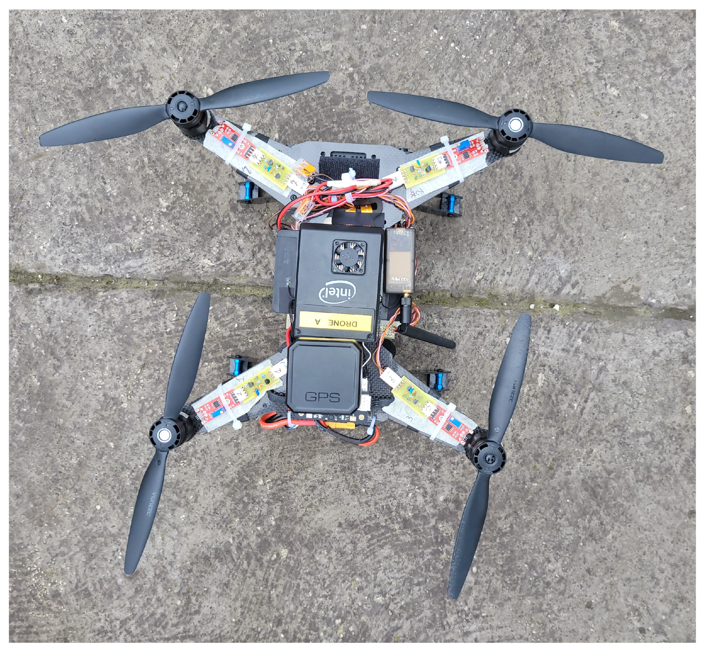
The drone used is a UAV development platform developed by Intel®Aero (total weight 1450 g, during tests), as shown in Figure 1. The platform includes an Intel Aero Compute Board for advanced computation such as video based navigation (mostly not used in the experimental validation test), four electric motors with their Electronic Speed Controller (ESC), a flight controller, and a sensor suite including the following sensors required to control the vehicle:
- a six degrees of freedom (three accelerometers and three gyroscopes) IMU (BMI160);
- a magnetometer (BMM150);
- an altimeter (MS5611);
- a GPS Receiver (u-blox Neo-M8N GPS/GLONASS receiver).
The flight controller runs a Flight Control Software Dronecode PX4. The basic Intel Aero configuration has been expanded for a limited number of fight tests with a custom setup that includes an angular speed sensor for each propeller. These additional sensors were required to validate the representativeness of the propeller angular speed estimate, available from the SW of the flight controller. In fact, these quantities in the basic configuration are not directly measured but estimated through the parameters of the ESC.
3.2. Flight Dynamics Results
In order to validate the flight dynamic model, experimental–numerical comparisons are performed. For three different trim conditions (hovering, climb, and forward flight) the angular velocities of the four rotors and the attitude angles of roll and pitch are shown. The experimental tests were carried out outdoors in Capua and from the online available weather data, it was possible to obtain information on the average intensity and direction of the wind, as shown in Figure 2, where the local reference system is shown in a solid line and the north-east reference system in a broken line. The plane of both references coincides with the ground.
3.2.1. Hovering
The hovering test was performed with the drone fixed in point of the local system, at an altitude of 3.5 m above the ground, pointing towards the local x axis. Graphical comparisons are shown below in Figure 3a,b and Table 1 below shows the percentage relative errors of the three models.
Already in this simple case, it can be seen that the three models give very different results between them, albeit following the same trend. As we can see, the 45 state model recovers the experimental results better, and the error increases as the number of the wake states decreases. In a hover condition without atmospheric wind one would expect to obtain very similar RPM values from the different models, as the total thrust is largely governed by the mean inflow on the rotor disk. In the presence of wind, as can be seen from the Figure A2a,b, as the number of states increases, the thrust generated by the rotors tends to decrease, with the same rotation speed. This is reflected in an increase in RPM to balance the weight of the drone. In general an underestimation of the angular speed of the propellers is observed from the numerical results. This trend can be justified by the fact that the blade has been modeled as rigid while in the real case the presence of negative blade aerodynamic pitching moment produces a pitch down blade torsion with a consequent reduction of the average angle of attack, which is compensated by the increase of the rotor angular speeds. In particular, the errors on the attitude angles are very high for the 0 × 0 Peters He model, due to its inability to correctly predict the rotor moments and side forces.
3.2.2. Climb
The same experimental–numerical comparisons were done for the climb condition. The drone starts from point at an altitude of 3.5 m above the ground and reaches a constant speed of about 4.6 m/s. Again the results and errors are shown below, in Figure 4a,b and Table 2.
Additionally, in this case, it is possible to make similar considerations: the best model is represented by the one with the highest number of states, and the angular speeds are underestimated by numerical results.
3.2.3. Forward
The last test was performed in forward flight, at a speed of 5 m/s and an altitude of 4.5 m from the ground, pointing towards the negative direction of the local y axis.
To better discuss the results of this case reported in Figure 5, Figure 6 shows the induced velocities of the four rotors, obtained with the 45 states model.
The increase in the Peters and He number of states produces a significant improvement in the accuracy of the predictions, especially for the attitude angles. Despite the deviation in the prediction of rotor angular speed, we observed a good agreement of the mean values and an underestimation for the rear rotors which is compensated by an overestimation for the front ones (Table 3). This is probably due to the approximations of the point of application of body airloads (modeled as equivalent flat plate), which may probably lead to a low agreement on the drone pitching moment. Figure 6 shows how the inflow distribution in forward flight is such that the front of the disk experiences less downwash than the rear of the disk, and the lateral distribution is such that the advancing side sees more downwash than the retreating side. From Figure A2 it can also be seen that higher order inflow models amplify this trend, increasing the downwash in the rear and advancing sides and decreasing it in the front and retreating sides. In the Peters and He model, the inflow is directly related to the lift distribution of the rotor, so that a greater inflow corresponds to a higher lift (this can also be seen as the effect of the induced velocity in deflecting the relative wind direction on the blade section, effectively increasing the angle of attack). This causes the drone to tilt in the direction from which the wind is coming, lowering both the pitch and roll angle. The 0 × 0 model fails to recover this lift distribution across the four rotors, leading to higher trim angle errors.
3.3. Aeroacoustics
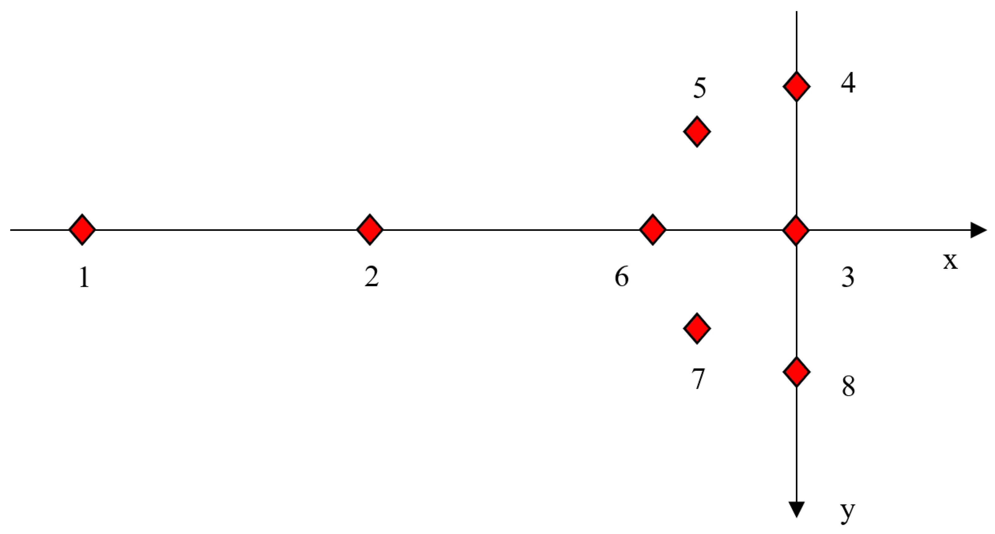
For the aeroacoustics validation the eight microphones sketched in Figure 7 were used. Their position are shown in local reference system in Table 4. In particular, the experimental–numerical comparisons are computed on the eight microphones for two hover conditions and for a forward flight. The microphones are positioned 1.5 m above the ground.
As mentioned in the introduction, the comparisons are shown in the frequency domain. From the graphs of the experimental results it is expected to observe the tonal noise values in correspondence of the blade pass frequencies (BPF), in the form of peaks that clearly deviate from the broadband noise, as simplified in Figure 8.
For the numerical results, the same behavior is expected, except for the absence of the broadband part, due to non-modeled interaction effects, electric motors, and background noise. Since each rotor has a different rotational speed, it is expected to have four peaks in correspondence to each BPF. Due to non-modeled interactional effects (between the rotors and with the ground) in the calculation of the aerodynamic forces, it is expected that only the first two BPF are correctly provided by the model [1]. The higher frequency noise content, although smaller, can affect the way it is perceived by humans, as hearing is biased towards high frequencies (>1000 Hz). Furthermore, at higher frequencies the noise produced by electric motors becomes increasingly important, up to the point of overcoming the contribution given by the propellers [6].
The experimental–numerical comparison graphs in the frequency domain can be found in Appendix C. In addition, the overall SPL values in the frequency ranges analyzed for the three cases are reported, comparing the experimental values with those obtained from Peters and He models with 15 and 45 states.
3.3.1. Hovering with Experimental Data
A first aeroacoustic comparison has been performed using experimental attitude and controls as input for the aeroacoustic solver, Table 5. The drone is positioned in and the first average BPF is equal to approximately 195 Hz.
Below, in Figure 9, are the experimental–numerical comparisons of the overall SPLs in the frequency range analyzed.
The difference between the experimental and numerical values is always less than 3 dB, except for the first two microphones which, being further away, are characterized by a lower noise level, considering that angle under which the observer sees the source is smaller. Conversely, the microphones placed under the drone have on average higher pressure values, since the loading noise acts the most under the plane of the rotors. As can be seen, increasing states from 15 to 45 does not result in a significant improvement in low-frequency noise prediction.
3.3.2. Forward with Experimental Data
The second test case is representative of a forward flight at 5 m/s. In particular, we examined the instant when the drone flies over microphone 3, pointing towards the negative direction of the local y axis. Experimental attitude and controls have been used as inputs for numerical calculations (Table 6). The first average BPF is equal to approximately 185 Hz.
Below, in Figure 10, are the experimental–numerical comparisons of the overall SPLs in the frequency range analyzed.
In this case, the numerical underestimation is greater than the hover case since the interactional effects increase due to the greater oscillation of the loads on the blades.
3.3.3. Hovering with Numerical Data
In this hovering comparison, the numerical analysis is complete on the entire aeropropulsive and aeroacoustic simulation chain. In particular, the values used in input to the aeroacoustic solver are obtained from the dynamics simulation discussed in Section 3.2.1, Table 7. This analysis is important due to the need to obtain noise predictions for strategic flight planning when online flight data is not available.
The graphs below show the comparison between the experimental results and the numerical ones, with the 15 and 45 Peters and He state models. The spectrum is reported down to about 530 Hz. The first average BPF is equal to approximately 193 Hz and the yaw angle is zero.
Below, in Figure 11, are the experimental–numerical comparisons of the overall SPLs in the frequency range analyzed.
Even if the correlations in this case are worse than the hover seen previously, the accuracy levels are still satisfactory, taking into account that the dynamics of the aircraft and rotors are numerically simulated.
4. Conclusions
In the present work, an integrated code for the aeropropulsive and aeroacoustics characterization of a quadcopter drone has been developed and validated through experimental data. The impact of the induced velocity on the attitude and commands in flight conditions has been evaluated using BET and the Peters and He dynamic wake model. It has been found that the 45 states of the Peters and He dynamic model give good adherence to the experimental results obtained for flight dynamics, in particular for the prediction of angular velocities and attitude in trim conditions. On the other hand, models with a few states in atmospheric wind conditions show quite high errors even in simple conditions such as hovering. For the aeroacoustics part, the 15 and 45 states models do not show evident differences between them, and both are able to correctly predict the tonal noise values up to the second BPF since the interactional effects of aerodynamics have not been modeled. In general is possible to observe a good agreement for the first BPF of each rotor and an underestimation for the second one. Since the proposed model is generalizable, the same procedure exhibited can also be applied to other types of rotary-wing aircraft, although new experimental–numerical comparisons should be made to evaluate the effect of the number of wake states. In order to obtain better correlations in the future, more attention will have to be paid to the airloads acting on the fuselage, through CFD simulation and using the drone 3D scanner, to correctly predict the moments acting on the fuselage in forward flight; the effects of elasticity of the blades can be considered to more accurately estimate the angles of attack of the blade sections; models for broadband noise can be added in the aeroacoustics model as well as models of unsteady aerodynamics, instead of only considering tonal noise in the OSPL estimate; new experimental tests may be carried out, in the absence of external disturbances, reducing as much as possible the effect of wind and background noise to obtain better comparisons and more easily generalizable analyses.
In conclusion, the integrated model developed has shown satisfactory results and, if appropriately improved, it is useful to evaluate the impact of design strategies on noise emitted by propellers, such as increasing the number of blades, optimizing the blade airfoil and planform shapes, modifying the rotor-airframe and inter-rotor distances and positions, manipulating the rotor phasing, etc. Furthermore, it is suitable for planning low-noise trajectory for drones in complex scenarios such as the urban one, both in the tactical phase, based on assets and commands acquired online during the flights, and in the strategic phase on the basis of simulated data.
Author Contributions
Conceptualization, L.F. and R.C.; Data curation, F.F. and L.F.; Formal analysis, F.F. and M.C.; Investigation, F.F., L.F. and M.C.; Methodology, L.F., M.C. and R.C.; Resources, L.F. and M.C.; Software, F.F. and M.C.; Supervision, L.F., M.C. and R.C.; Visualization, F.F.; Writing—original draft, F.F.; Writing—review & editing, F.F., M.C. and R.C. All authors have read and agreed to the published version of the manuscript.
Funding
This research received no external funding.
Institutional Review Board Statement
Not applicable.
Informed Consent Statement
Not applicable.
Data Availability Statement
Not applicable.
Conflicts of Interest
The authors declare no conflict of interest.
Abbreviations
The following abbreviations are used in this manuscript:
| ACP | Aerodynamic Computational Points |
| BET | Blade Element Theory |
| BPF | Blade Pass Frequency |
| CFD | Computational Fluid Dynamics |
| CCW | Counterclockwise |
| CW | Clockwise |
| SPL | Sound Pressure Level |
| UAM | Urban Air Mobility |
Appendix A. Blade’s Geometry and Properties
The blade’s chord and pitch along the radius are shown in Figure A1a,b below.
Figure A1.
Blade geometry.

The blade’s properties are shown in Table A1 below.

Table A1.
Blade properties.
| Length | Weight | Density | Hub Diameter |
|---|---|---|---|
Appendix B. Peters and He Model Results
From Figure A2a,b below, in which the thrust values versus time are reported for four different wake models (at a fixed rotational speed), it is possible to see how, integrating every degree of blade’s rotation, the solution converges and becomes periodic after a few (about 2) complete revolutions. In general, it can be seen that few-state models tend to predict a higher average value of thrust.
In Figure A2 are graphical results for three different forward flight conditions and two different wake models, respectively with 15 and 45 total states. In particular, the values of the induced velocity on the disk are shown, for a counterclockwise (CCW) rotor rotating at 525 rad/s (wind blowing from the left).
Figure A2.
CCW Rotor, Induced Velocity.


It is possible to observe an increase in the reverse flow size region and of the maximum downwash in the blade advancing side when the number of Peters and He states is increased.
Appendix C. Aeroacoustics Results Comparisons
Figure A3.
Experimental–Numerical Comparison—Hover Numerical data.


References
- Smith, B.; Healy, R.; Gandhi, F.; Lyrintzis, A. eVTOL Rotor Noise in Ground Effect. In Proceedings of the Vertical Flight Society’s 77th Annual Forum & Technology Display, Online, 10–14 May 2021. [Google Scholar]
- Rizzi, S.A.; Huff, D.L.; Boyd, D.D.J.; Bent, P.; Henderson, B.S.; Pascioni, K.A.; Sargent, D.C.; Josephson, D.L.; Marsan, M.; He, H.; et al. Urban Air Mobility Noise: Current Practice, Gaps, and Recommendations; NASA Langley Research Center: Hampton, VA, USA, 2020.
- Pagano, A.; Barbarino, M.; Casalino, D.; Federico, L. Tonal and broadband noise calculations for aeroacoustic optimization of a pusher propeller. J. Aircr. 2010, 47, 835–848. [Google Scholar] [CrossRef]
- Brooks, T.F.; Schlinker, R.H. Progress in rotor broadband noise research. Vertica 1983, 7, 287–307. [Google Scholar]
- Glegg, S.A.L.; Glendinning, S.M.B.A.G. The prediction of broadband noise fromwind turbines. J. Sound Vib. 1987, 118, 217–239. [Google Scholar] [CrossRef]
- Vieira, A.; Cruz, L.; Lau, F.; Mortagua, J.P.; Santos, R. A New Computational Framework for UAV Quadrotor Noise Prediction. In Proceedings of the 5th CEAS Air & Space Conference, Delft, The Netherlands, 7–11 September 2015. [Google Scholar]
- Ffowcs-Williams, J.E.; Hawkings, D.L. Sound generation by turbulence and surfaces in arbitrary motion. Philos. Trans. R. Soc. 1969, 264, 321–342. [Google Scholar]
- Quan, Q. Introduction to Multicopter Design and Control; Springer Nature: Singapore, 2020. [Google Scholar]
- Niemiec, R.; Gandhi, F. Effects of Inflow Model on Simulated Aeromechanics of a Quadrotor Helicopter; American Helicopter Society International, Inc.: Fairfax, VA, USA, 2016. [Google Scholar]
- Niemiec, R.; Gandhi, F. Development and Validation of the Rensselaer Multicopter Analysis Code (RMAC): A Physics-Based Comprehensive Modeling Tool. In Proceedings of the Vertical Flight Society 75th Annual Forum & Technology Display, Philadelphia, PA, USA, 13–16 May 2019. [Google Scholar]
- Pounds, P. Design of a Four-Rotor Aerial Robot. In Proceedings of the Australasian Conference on Robotics and Automation, Auckland, Australia, 27–29 November 2002. [Google Scholar]
- Erginer, B.; Altug, E. Modeling and PD Control of a Quadrotor Vehicle. In Proceedings of the IEEE Intelligent Vehicles Symposium, Istanbul, Turkey, 13–15 June 2007. [Google Scholar]
- Mueller, M.; D’Andrea, R. Stability and Control of a Quadrocopter Despite the Complete Loss of One, Two, or Three Propellers. In Proceedings of the IEEE International Conference on Robotics and Automation, Hong Kong, China, 31 May–7 June 2014. [Google Scholar]
- Yoon, S.; Diaz, P.; Boyd, D.D.; Chan, W.; Theodore, C. Computational Aerodynamic Modeling of Small Quadcopter Vehicles. In Proceedings of the 73rd Annual Forum of the American Helicopter Society International, Fort Worth, TX, USA, 8–11 May 2017. [Google Scholar]
- Misiorowski, M.; Gandhi, F.; Oberai, A. A Computational Study on Rotor Interactional Effects for a Quadcopter in Edgewise Flight. In Proceedings of the 74th Annual Forum of the American Helicopter Society, Phoenix, AZ, USA, 14–17 May 2018. [Google Scholar]
- Bramwell, A.R.S.; Done, G.; Balmford, D. Bramwell’s Helicopter Dynamics; Butterworth-Heinemann: Oxford, UK, 2001. [Google Scholar]
- Padfield, G.D. Helicopter Flight Dynamics; Blackwell Science Ltd.: Oxford, UK, 1996. [Google Scholar]
- Leishman, J.G. Principles of Helicopter Aerodynamics; Cambridge University Press: New York, NY, USA, 2000. [Google Scholar]
- Fay, G. Derivation of the Aerodynamic Forces for the Mesicopter Simulation; Stanford University: Stanford, CA, USA, 2001. [Google Scholar]
- Glauert, H. The Elements of Aerofoil and Airscrew Theory; Cambridge University Press: Cambridge, UK, 1926. [Google Scholar]
- Hoydonck, W.R.M.V.; Haverdings, H.; Pavel, M.D. A review of rotorcraft wake modeling methods for flight dynamics applications. In Proceedings of the 35th European Rotorcraft Forum, Hamburg, Germany, 22–25 September 2009. [Google Scholar]
- Mangler, K.W.; Squire, H.B. The induced velocity field of a rotor. In Aeronautical Research Council Reports and Memoranda; Her Majesty’s Stationery Office: London, UK, 1953. [Google Scholar]
- Peters, D.A.; Boyd, D.D.; He, C.J. Finite-State Induced-Flow Model for Rotors in Hover and Forward Flight. In Proceedings of the 43rd Annual Forum of the American Helicopter Society, St. Louis, MO, USA, May 18–20 1987. [Google Scholar]
- Peters, D.A.; He, C.J. Finite State Induced Flow Models Part II: Three-Dimensional Rotor Disk. J. Aircr. 1995, 32, 323–333. [Google Scholar] [CrossRef]
- Pitt, D.M.; Peters, D.A. Theoretical Prediction of Dynamic—Inflow Derivatives. Vertica 1981, 5, 21–34. [Google Scholar]
- Pitt, D.M.; Peters, D.A. Rotor Dynamic Inflow Derivatives and Time Constants from Various Inflow Models. In Proceedings of the Ninth European Rotorcraft Forum, Stresa, Italy, 13–15 September 1983. [Google Scholar]
- Carpenter, P.J.; Fridovitch, B. Effect of Rapid Blade-Pitch Increase on the Thrust and Induced Velocity Response of a Full-Scale Helicopter Rotor; NACA: Langley Field, VA, USA, 1953. [Google Scholar]
- Drees, J.M., Jr. A Theory of Airflow Through Rotors and its Application to Some Helicopter Problems. J. The Helicopter Assoc. Great Br. 1949, 3, 79–104. [Google Scholar]
- FLIGHTLAB Theory Manual (Vol. One); Advanced Rotorcraft Technology: Sunnyvale, CA, USA, 2011.
- FLIGHTLAB Theory Manual (Vol. Two); Advanced Rotorcraft Technology: Sunnyvale, CA, USA, 2011.
- Bauchau, O.A. Dymore User’s Manual; School of Aerospace Engineering, Georgia Institute of Technology: Atlanta, GA, USA, 2007. [Google Scholar]
- Delfs, J. Basics of Aeroacoustics; DLR-German Aerospace Center: Braunschweig, Germany, 1996. [Google Scholar]
- Wang, Y.; Göttsche, U.; Abdel-Maksoud, M. Sound Field Properties of Non-Cavitating Marine Propellers. J. Mar. Sci. Eng. 2020, 8, 885. [Google Scholar] [CrossRef]
- Lummer, M.; Richter, C.; Prober, C.; Delfs, J. Validation of a Model for Open Rotor Noise Predictions and Calculation of Shielding Effects Using a Fast BEM; American Institute of Aeronautics and Astronautics: Reston, VA, USA, 2013. [Google Scholar]
- Rienstra, S.W.; Hirschberg, A. An Introduction to Acoustics; Eindhoven University of Technology: Eindhoven, The Netherlands, 2021. [Google Scholar]
- Farassat, F. Linear acoustic formulas for calculation of rotating blade noise. AiAA J. 1981, 19, 1122–1130. [Google Scholar] [CrossRef]
- Farassat, F.; Succi, G.P. A review of propeller discrete frequency noise prediction technology with emphasis on two current methods for time domain calculations. J. Sound Vib. 1980, 71, 399–419. [Google Scholar] [CrossRef]
- Farassat, F.; Brentner, K.S. The acoustic analogy and the prediction of the noise of rotating blades. Theor. Comput. Fluid Dyn. 1998, 10, 155–170. [Google Scholar] [CrossRef]
- Farassat, F. Derivation of Formulations 1 and 1A of Farassat; NASA Langley Research Center: Hampton, VA, USA, 2007.
- Brentner, K.S.; Farassat, F. An Analytical Comparison of the Acoustic Analogy and Kirchhoff Formulation for Moving Surfaces; NASA Langley Research Center: Hampton, VA, USA, 1997.
- Succi, G.P.; Munro, D.H.; Zimmer, J.A. Experimental verification of propeller noise prediction. AiAA J. 1980, 20, 1483–1491. [Google Scholar] [CrossRef]
- Marino, L. Experimental analysis of UAV-propeller noise. In Proceedings of the 16th AIAA/CEAS Aeroacoustic Conference, Stockholm, Sweden, 7–9 June 2010. [Google Scholar]
- Sinibaldi, G.; Marino, L. Experimental analysis on the noise of propellers for small UAV. Appl. Acoust. 2013, 74, 79–88. [Google Scholar] [CrossRef]
- Etkin, B. Dynamics of Atmospheric Flight; John Wiley & Sons: Toronto, ON, Canada, 1972. [Google Scholar]
Figure 1.
Experimental setup—drone.

Figure 2.
Wind components.

Figure 3.
Experimental–Numerical Comparison, Hovering.

Figure 4.
Experimental–Numerical Comparison, Climb.

Figure 5.
Experimental–Numerical Comparison, Forward.

Figure 6.
Induced velocities in forward flight (m/s).

Figure 7.
Microphones’ positions.

Figure 8.
Tonal and broadband noise.

Figure 9.
Experimental–Numerical Comparison—Hover Exp—OSPL.

Figure 10.
Experimental–Numerical Comparison—Forward—OSPL.

Figure 11.
Experimental–Numerical Comparison—Hover Num—OSPL.

Table 1.
Percent Error—Hovering.
| Roll | Pitch | Rotor 1 | Rotor 2 | Rotor 3 | Rotor 4 | |
|---|---|---|---|---|---|---|
| 0 × 0 model | −33.53% | −34.31% | −6.65% | −5.81% | −8.03% | −9.46% |
| 4 × 4 model | −3.44% | 7.01% | −3.74% | −2.50% | −4.82% | −5.19% |
| 8 × 8 model | −0.86% | −0.53% | −0.75% | −0.78% | −2.75% | −2.74% |
Table 2.
Percent Error—Climb at 4.6 m/s.
| Roll | Pitch | Rotor 1 | Rotor 2 | Rotor 3 | Rotor 4 | |
|---|---|---|---|---|---|---|
| 0 × 0 model | 10.79% | 18.27% | −6.07% | −10.06% | −12.03% | −13.27% |
| 4 × 4 model | 6.66% | 6.57% | −0.35% | −3.05% | −5.95% | −6.72% |
| 8 × 8 model | 5.41% | 4.05% | 3.20% | 0.00% | −2.45% | −3.35% |
Table 3.
Percent Error—Forward at 5 m/s.
| Roll | Pitch | Rotor 1 | Rotor 2 | Rotor 3 | Rotor 4 | |
|---|---|---|---|---|---|---|
| 0 × 0 model | −24.39% | −16.20% | 7.33% | −11.20% | 4.02% | −10.97% |
| 4 × 4 model | −1.95% | −2.23% | 7.80% | −6.99% | 4.17% | −6.56% |
| 8 × 8 model | −1.66% | −1.24% | 9.29% | −5.56% | 5.26% | −5.34% |
Table 4.
Microphones’ positions.
| Microphone | x (m) | y (m) | z (m) |
|---|---|---|---|
| 1 | −15 | 0 | 1.5 |
| 2 | −9 | 0 | 1.5 |
| 3 | 0 | 0 | 1.5 |
| 4 | 0 | −3 | 1.5 |
| 5 | −2.12 | −2.12 | 1.5 |
| 6 | −3 | 0 | 1.5 |
| 7 | −2.12 | 2.12 | 1.5 |
| 8 | 0 | 3 | 1.5 |
Table 5.
Hovering with experimental data.
| Roll (deg) | Pitch (deg) | Yaw (deg) | Rotor 1 (rpm) | Rotor 2 (rpm) | Rotor 3 (rpm) | Rotor 4 (rpm) |
|---|---|---|---|---|---|---|
| −1.98 | 0.30 | −129.93 | 5562 | 5882 | 5751 | 6164 |
Table 6.
Forward with experimental data.
| Roll (deg) | Pitch (deg) | Yaw (deg) | Rotor 1 (rpm) | Rotor 2 (rpm) | Rotor 3 (rpm) | Rotor 4 (rpm) |
|---|---|---|---|---|---|---|
| 0.19 | −5.69 | −79.23 | 4595 | 6035 | 4621 | 6210 |
Table 7.
Hovering with numerical data.
| Roll (deg) | Pitch (deg) | Rotor 1 (rpm) | Rotor 2 (rpm) | Rotor 3 (rpm) | Rotor 4 (rpm) | |
|---|---|---|---|---|---|---|
| Experimental | −1.62 | 1.28 | 5706 | 5744 | 5743 | 5998 |
| 4 × 4 model | −1.57 | 1.38 | 5501 | 5604 | 5479 | 5702 |
| 8 × 8 model | −1.61 | 1.27 | 5664 | 5699 | 5589 | 5838 |
Publisher’s Note: MDPI stays neutral with regard to jurisdictional claims in published maps and institutional affiliations. |
© 2022 by the authors. Licensee MDPI, Basel, Switzerland. This article is an open access article distributed under the terms and conditions of the Creative Commons Attribution (CC BY) license (https://creativecommons.org/licenses/by/4.0/).
Share and Cite
MDPI and ACS Style
Fruncillo, F.; Federico, L.; Cicala, M.; Citarella, R. Development and Validation of an Aeropropulsive and Aeroacoustic Simulation Model of a Quadcopter Drone. Drones 2022, 6, 143. https://doi.org/10.3390/drones6060143
AMA Style
Fruncillo F, Federico L, Cicala M, Citarella R. Development and Validation of an Aeropropulsive and Aeroacoustic Simulation Model of a Quadcopter Drone. Drones. 2022; 6(6):143. https://doi.org/10.3390/drones6060143
Chicago/Turabian StyleFruncillo, Felice, Luigi Federico, Marco Cicala, and Roberto Citarella. 2022. "Development and Validation of an Aeropropulsive and Aeroacoustic Simulation Model of a Quadcopter Drone" Drones 6, no. 6: 143. https://doi.org/10.3390/drones6060143