
Robust Path-Following Control for AUV under Multiple Uncertainties and Input Saturation

School of Ocean Engineering and Technology, Sun Yat-sen University, Southern Marine Science and Engineering Guangdong Laboratory (Zhuhai), Zhuhai 519000, China
*
Author to whom correspondence should be addressed.
Drones 2023, 7(11), 665; https://doi.org/10.3390/drones7110665
Submission received: 3 October 2023
/
Revised: 1 November 2023
/
Accepted: 2 November 2023
/
Published: 8 November 2023
Abstract
:In this paper, a robust path-following control strategy is proposed to deal with the path-following problem of the underactuated autonomous underwater vehicle (AUV) with multiple uncertainties and input saturation, and the effectiveness of the proposed control strategy is verified by semi-physical simulation experiments. Firstly, the control laws are constructed based on the traditional backstepping method; the multiple uncertainties are treated as lumped uncertainties, which can be estimated and eliminated by the employed extended state observers (ESOs). In addition, the influence of input saturation can be compensated by the designed auxiliary dynamic compensators. Secondly, to simplify controller design and address the “complexity explosion”, two command filters are used to obtain the estimated value of the unknown sideslip angular velocity and the desired yaw angular acceleration, respectively. Finally, the superiority and robustness of the proposed control strategy are verified through computer simulation. A semi-physical simulation experiment platform is built based on the NI Compact cRIO-9068 and PLC S7-1200 to further demonstrate the effectiveness of the proposed control strategy.
1. Introduction
In decades, the development of marine resources and marine exploration have developed rapidly. Unmanned underwater vehicles (UUVs) have the characteristics of flexible operation, strong autonomy in decision making, and deep intelligence, which have attracted much attention when completing certain tasks underwater [1,2,3]. However, due to underactuation, high nonlinearity, and coupling effects, achieving precise motion control in autonomous underwater vehicles (AUVs) remains a challenging task [4,5]. Furthermore, multiple uncertainties, such as internal parameter uncertainties, unknown environmental disturbances, and unmodeled dynamics, are widespread and inevitable in engineering practice, which may lead to performance degradation [6,7].
In recent years, there have been significant advancements in AUV motion control research, such as the backstepping control method [8,9], the sliding mode control (SMC) method [10,11], the disturbance observer-based control (DOBC) method [12,13], etc. To achieve better control performance, multiple methods are usually combined. In [14], the integral SMC and RBFNN are used to address modeling errors and unknown disturbances. In [15], a backstepping SMC based on an adaptive slow-varying observer was designed to estimate and eliminate the multiple disturbances. In [16], a neural network-based state observer is designed and a finite time controller is designed using backstepping and command filtering techniques to realize the finite time adaptive tracking control problem for AUVs. In [7], the H∞ control method is combined with the DOBC method to deal with the multiple disturbances according to their main characteristics. In addition, guidance law is irreplaceable in the design of motion controllers [17]. The line-of-sight (LOS) guidance scheme is simple and can mimic trained sailors [18], which has been widely used in driving the AUVs to converge to the desired path [7,19,20,21]. In [5], a LOS guidance law based on an indirect adaptive DO and an adaptive look-ahead distance was proposed, which enables the AUV to follow the curved path with sharp turning. In [22], an LOS guidance law based on the fixed-time predictor is designed to enable the underactuated USV with unknown disturbances to track the desired path. In [23], an ESO-based integral LOS with an adaptive fuzzy integral SMC scheme is proposed to deal with the problem of path following for underactuated USVs. It should be pointed out that input saturation is also a non-negligible problem in practical applications. If the influence of input saturation is not considered, the designed control strategy may lead to a degradation in system performance or even instability [24,25]. To address this issue, an auxiliary dynamic compensator is designed [26], and the auxiliary variable is brought into the design of the dynamic controller to limit the control input. In [27], formation control under input constraints is realized by employing the saturation function in a kinematics loop design. In addition, disturbances and input saturation have been simultaneously considered in the control of the quadrotor unmanned aerial vehicle (UAV). In [28], a fixed-time DO-based robust fault-tolerant tracking control scheme is used to drive the UAV to track a presupposed trajectory under the simultaneous existence of model uncertainties, external disturbances, actuator faults, and input delay. In [29], to achieve tracking control of the quadrotor UAV under disturbance and input saturation, the DO-based state estimator is used to tackle the disturbances, and the filtering error compensation mechanism, auxiliary control system, and first-order sliding mode differentiator are combined to address the adverse effects of filtering errors, input saturation, and the computing complexity problem. Therefore, constructing a high-performance path-following control strategy for AUVs that considers both the multiple uncertainties and input saturation is meaningful but challenging.
Physical experiments have always been the most direct means of verifying the effectiveness of control algorithms. However, the experimental cost is high, the cycle is long, and there is a possibility of being damaged by natural risks, which is not conducive to daily learning and research. Another noteworthy aspect is that semi-physical simulation experiments can simulate the interaction and collaboration of different subsystems to verify the stability and reliability of the system, which has been widely applied in various fields. In [30], a virtual hybrid power system was constructed to use a virtual controller to control the real motor. In [31], the speed control performance between anti-wind PI controllers and traditional PI controllers based on Scilab/Scicoslab was compared, and hardware simulations on the brushless DC motor were conducted. In [32], aiming at the hardware in the loop simulation test process of aircraft landing point coordinates, the concept of a data integrity test of landing point simulation was proposed, and an integrity test oracle machine based on field test data and expert estimation information was constructed. In addition, a semi-physical simulation experiment is important in the design, development, and testing processes of AUVs, which have been widely used in the field of AUVs [33,34]. By combining real physical devices with virtual models, it is possible to simulate and evaluate the performance and feasibility of different design options. In the development process of AUVs, multiple subsystems need to be integrated and work together, such as navigation systems, sensor systems, and communication systems. As a consequence, it is also very meaningful to build a semi-physical simulation experiment platform for AUVs to further verify the effectiveness of the proposed control strategy.
Considering the aforementioned challenges, this paper proposes a new robust control strategy for underactuated AUVs under multiple uncertainties and input saturations and demonstrates the effectiveness of the proposed control strategy through semi-physical simulation experiments. The main contributions of this paper can be summarized as follows:
- (1)
- A robust controller is constructed to achieve the path-following control of the underactuated AUV with multiple uncertainties and input saturation. The multiple uncertainties, including external environmental disturbances, internal uncertainties, and unmodeled dynamics, are treated as lumped uncertainties, and then the ESOs are employed to estimate and eliminate them. The input saturation constraints are compensated by the auxiliary dynamic compensators. In addition, two command filters are employed to simplify controller design and address the “complexity explosion”. Distinct from the previous literature, both the multiple uncertainties and input saturation are considered in this paper, which makes the designed control strategy more suitable for complex marine environments;
- (2)
- A semi-physical simulation experiment platform is built to further validate the effectiveness of the proposed control algorithm. The underactuated AUV actuators are connected to the control system, and the real-time data of the actuators is read by the NI Compact cRIO-9068 real-time control computer and PLC S7-1200 industrial control computer. A human–machine interaction interface is developed based on LabVIEW, which visualizes the simulation results and can intuitively display information such as AUV position and velocity. Compared with computer simulation, semi-physical simulation experiments involve actual actuators, which can verify the effectiveness of the control strategy on actual hardware devices and reduce uncertainties caused by differences between theoretical models and actual systems.
The remaining parts are arranged as follows. The model and error dynamics of the underactuated AUV are given in Section 2. The designed control laws are explained in Section 3. Stability analysis is introduced in Section 4. The computer simulation and semi-physical simulation experiments are shown in Section 5 and Section 6, respectively. The main work of this paper is summarized in Section 7.
2. Problem Formulation
2.1. Underactuated AUV Model in the Horizon Plane
The movement of the underactuated AUV in the horizon plane can be expressed by kinematic equations [5]:
where denotes the generalized position vector of the underactuated AUV in the inertial frame; and denotes the velocity vector of the underactuated AUV in the body-fixed frame.
Thor I. Fossen pointed out that wind and waves can be treated as generalized forces that can be directly added to nonlinear equations of motion [6]. Although the forces on a marine craft due to ocean currents are generally described by the relative velocity vector, K.D.Do proved that the force and moment produced by ocean current can be added to the nonlinear motion equation represented by the absolute velocity vector [35]. Therefore, the forces and moments produced by wind, waves, and currents are considered in the dynamic model and then treated as uncertainties in this paper. In addition, input saturation is an inevitable problem in practical engineering applications [24]. Hence, the control inputs should meet the following conditions: , where and denote the maximum and minimum values of the control input , respectively. Therefore, considering the multiple disturbances and input saturation, the dynamic model of the AUV can be represented as:
where , , and denote the total mass term of AUV, denotes the mass and denote the rotational inertia, respectively; , , , , , , , , and represent the hydrodynamic coefficients on different degrees of freedom; and denote the actual control input signal; and , , and denote the dynamic lumped uncertainties.
Assumption 1
Assumption 2
Remark 1:
Firstly, during normal operation of the AUV, external disturbances are limited. In addition, the internal uncertainties and unmodeled dynamics of the AUV are usually small. Assumption 1 is reasonable. Secondly, the underactuated AUV adopted in this paper is equipped with a variety of sensors, such as the Attitude and Heading Reference System (AHRS), Doppler Velocity Log (DVL), and Inertial Navigation System (INS). The AHRS is used to measure the attitude of the AUV, such as yaw angles. The DVL is used to measure the velocities of the AUV, such as surge and sway. The INS is used to measure the position of the AUV. Assumption 2 is practical.
2.2. The Error Dynamics Model
The control objective of path-following control is to drive the underactuated AUV to follow an arbitrary target point in a desired curve without time information. The desired curve can be expressed by a parameter , the path-tangential angle at point F is expressed as follows [39]:
where and are the positional coordinates of the point F, and and are the partial derivatives of and , respectively.
Assumption 3:
Remark 2:
AUVs are typically designed for tasks and data collection in underwater environments. To ensure the stability and accuracy of the AUV, its path needs to be smooth and finite.
Then, the error dynamic equation can be expressed as follows [40]:
where and and are the along-track error and cross-track error, respectively; denotes the angle tracking error; denotes the sideslip angle; and represents the total velocity.
The control objective of this paper is to design the control input and in Equation (2) to make the path-following errors and in Equation (4) rapidly converge to the neighborhood of zero.
3. Control Law Design
In this subsection, a robust path-following control strategy for the AUV under multiple uncertainties and input saturation is constructed, as shown in Figure 1, which can be divided into three components: LOS guidance law, kinematic control law, and dynamic control law. The LOS guidance law is constructed to calculate the desired yaw angle . In the kinematic control law, the virtual yaw angular velocity is proposed and the virtual surge velocity is given. In the dynamic control law, the designed ESOs are used to obtain the estimated value of the lumped uncertainties (, , and ), where the values ( and ) are used in designing the control inputs ( and ). To address the “explosion of complexity”, the command filters are employed to obtain the estimated value of the unknown sideslip angular velocity , virtual yaw angular velocity , and its derivative . In addition, the input saturations can be compensated by the auxiliary dynamic compensators.
3.1. The Design of the LOS Guidance Law
Considering the characteristics of simplicity and small computational footprint, the traditional proportional LOS guidance law is selected to generate the desired yaw angle
where represents the desired yaw angle and is the lookahead distance.
3.2. The Design of the Kinematic Control Law
For defining , , and . Equation (4) can be rewritten as follows:
where and .
Based on the Lyapunov direct method and the designed LOS guidance law, the kinematic control law for Equation (6) is proposed as follows:
where and are the control gains, which will be designed later. It should be pointed out that the constraint of the initial position is released by introducing an extra degree of freedom . To reduce the computational complexity, the command filter is used to obtain the estimated value of the sideslip angular velocity. Therefore, the kinematic control law for Equation (7) can be rewritten as follows:
where is the output of the command filter, which will be designed later.
3.3. The Design of Dynamic Control Law
Since the internal parameter uncertainties, environmental disturbances, and unmodeled dynamics are unknown, ignoring them will have a significant impact on control performance. In this subsection, the linear superposition of the multiple disturbances mentioned above is regarded as the lumped uncertainty, which can be estimated and eliminated by the designed ESOs. Finally, based on the designed ESO, the dynamic control law is derived.
The specific form of ESOs can be found in [4,35]. In previous studies [41,42], the error between the estimated values of the ESOs and the actual values for lumped disturbances has been proven to be bounded. Using the estimated value of and from the ESO, an anti-disturbance control law is proposed as:
where and are the controller gains to be designed. It should be noticed that the derivative ( and ) of the virtual command ( and ) is involved in Equation (12). To reduce the computational complexity, the desired surge velocity is given [43]. In addition, to handle the problem of “explosion of complexity”, the command filters are introduced to obtain the derivative of the desired yaw angular velocity. The command filters are constructed as follows [44]:
where is the input command signal, is the filtered signal of the input signal , is the derivative of , and the specific definitions of and can be found in [44]. It should be noted that, according to [44,45], the command filter technique can be introduced to obtain estimated values for their derivatives without affecting the system’s stability.
In addition, to compensate for the influence of input saturation, the auxiliary dynamic compensator designed in [7,46] is adopted in this paper. According to the outputs ( and ) of the command filter, the dynamic control law can be reorganized as follows:
where and denote the state of the designed auxiliary dynamic compensators; the detailed descriptions can be found in [7,46].
4. Stability Analysis
In this subsection, under Assumptions 1, 2, and 3, the whole control system formed by the guidance control law (5), the kinematic control law (8), the command filter (10), and the dynamic control law (11) is input-to-state stable. In addition, the tracking errors are uniformly and ultimately bounded, and the control performance can be improved by selecting control parameters.
Proof:
Considering a Lyapunov function as follows:
According to Equations (6) and (8), the time derivative of Equation (12) is attained by:
where , , .
And then, considering the following Lyapunov function:
According to Equations (2), (8), and (11), the time derivative of Equation (14) is attained by:
The next relation can be derived by using Young’s inequality [47]:
where , , , , , , , , , and , .
Solving the inequality (16) gives:
Therefore, the tracking errors and can be ultimately uniformly bound by selecting parameters to satisfy: , , , , , and . □
5. Computer Simulation Analysis
To demonstrate the superiority and robustness of the proposed control strategy, the performance is compared with the conventional backstepping approach proposed in [43] and the sliding mode approach proposed in [48,49] under multiple uncertainties and input saturation. Relevant parameters of AUV fluid dynamics can be referred to [7,20,50]. The AUV is driven to follow a curved path, and the corresponding parameters of the desired path can also be found in [20,43,51]. The lumped uncertainties , , and are assumed as follows:
The underactuated AUV’s initial conditions are chosen as follows: , , , , , , , and . The preset ranges of the saturation limit are , , , and . The underactuated AUV’s control parameters are designed as follows: , , , , , , , , , and , .
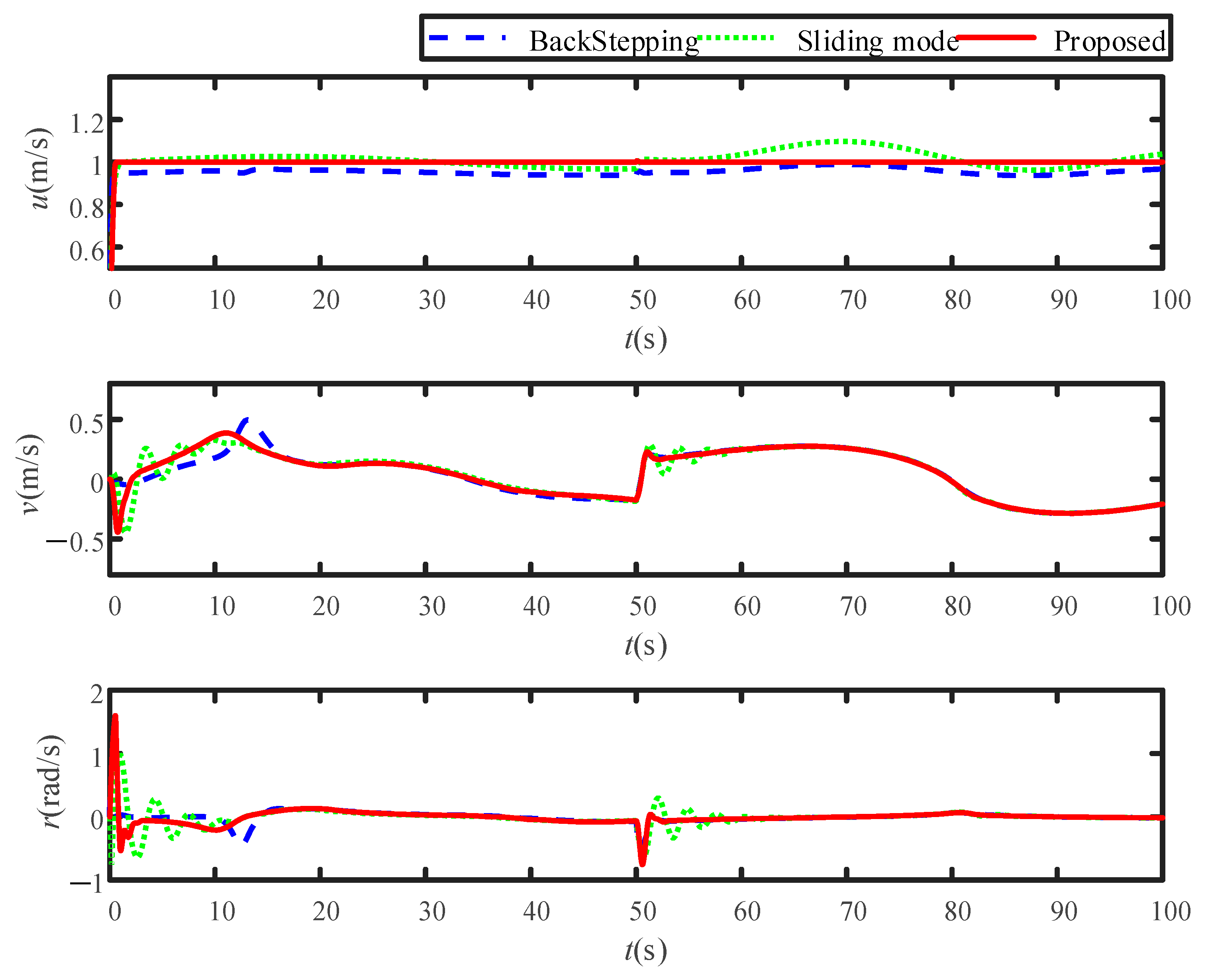
The simulation results are shown in Figure 2, Figure 3, Figure 4, Figure 5 and Figure 6. Figure 2 indicates that all three controllers can drive the AUV to follow the desired curve, and the performance of the proposed controller is superior to the other two controllers. Figure 3 shows that the path-following errors of all three controllers can converge to the neighborhood of zero, but there is a smaller following error under the proposed controller. From Figure 2 and Figure 3, it can be seen that the path-following errors under the proposed controller are smaller than the other two controllers. That is, the controller proposed in this paper has smaller steady-state errors and higher path-following accuracy. Figure 4 shows that the surge velocity and the yaw angular velocity of all three controllers converge to the desired speed in a short time. However, compared with the conventional backstepping controller and the sliding mode controller, the proposed controllers show better steady-state performance. The actual control inputs are expressed in Figure 5. The maximum capability of the AUV in this paper is 500 N. It is not difficult to see that the actual control inputs under the proposed controller always remain within the maximum capability of the AUV, which is attributed to the consideration of the input saturation constraint, whereas the control inputs under the other two controllers exceed the maximum capability, which cannot be achieved in practical engineering. The actual value and estimated value are illustrated in Figure 6. The results expressed that ESOs can accurately estimate the lumped uncertainties , , and , and the outputs (, , and ) of the command filters quickly converge to the desired commands (, , and ), respectively. It should be pointed out that after adding model parameter uncertainties to the lumped uncertainties, the proposed controller responds quickly and its control performance is almost unaffected, while the sliding mode controller requires a longer adjustment time, which proves the robustness of the proposed controller.
In addition, to evaluate the control performance of different methods more fairly and objectively, refer to [28,52], we have added four evaluation indicators in this paper, i.e., mean squared errors of position (MSEp), mean squared errors of attitude (MSEa), mean squared errors of surge velocity (MSEu), and mean squared errors of yaw angular velocity (MSEr). The values of the above performance indices are presented in Table 1 to better explain the superiority of the proposed controller.
6. Semi-Physical Simulation Experiment
6.1. Hardware Part
Hardware is a physical system in semi-physical simulation experiments, which is very important for the whole system. Based on the above computer simulation, a semi-physical simulation experiment platform is built to connect the underactuated AUV actuators to the control system. The real-time data of the actuators is read by the NI Compact cRIO-9068 real-time control computer and the PLC S7-1200 industrial control computer. The hardware structure of the semi-physical simulation experiment system is shown in Figure 7.
Next, a detailed description of the main hardware will be provided.
6.1.1. Propeller
The Siemens V90 is a standard model launched by Siemens worldwide that can achieve external pulse position control, internal setpoint position control, speed, and torque control and can meet various requirements. In addition, the motor is equipped with a standard braking resistor. The diversity and high integration of the Siemens V90 make it more cost-effective. Therefore, the Siemens V90 is selected as the propeller of the underactuated AUV, as shown in Figure 8.
6.1.2. Rudder
The rudder of the underactuated AUV adopts the Feite rudder SM150, which can be installed at any angle and can dynamically monitor data through software. The commands of the real-time simulation computer are collected by the RS485 bus and then processed by the motion controller to generate control signals to control the motor. The rudder is shown in Figure 9.
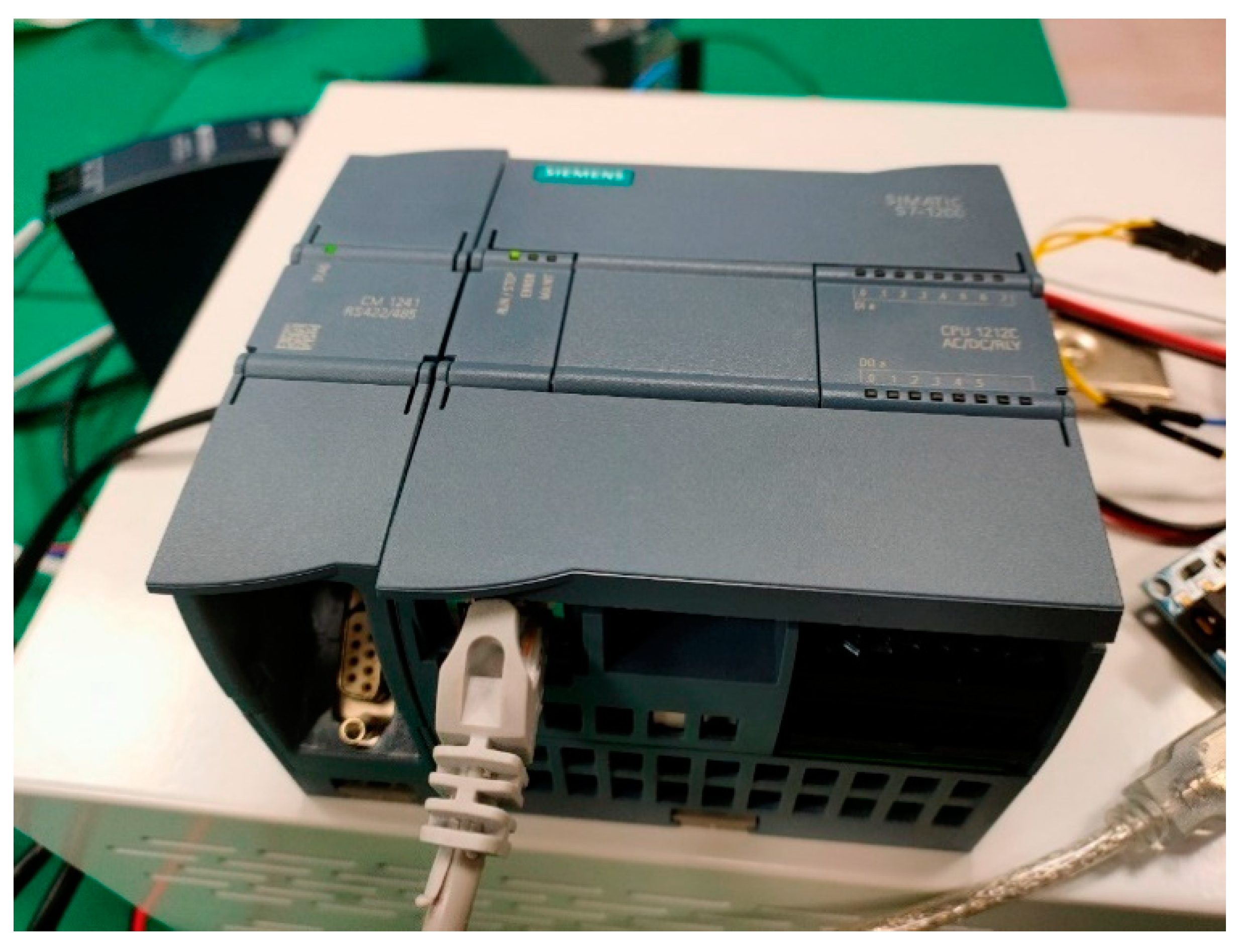
6.1.3. PLC S7-1200
PLC S7-1200 is selected as the controller of the underactuated AUV propeller, which is connected to the controller of the propeller through the network port, can convert the expected thrust generated by the control algorithm into speed and send it to the propeller in real-time, and can read the real-time speed generated by the thruster. The PLC S7-1200 selected in this article is shown in Figure 10.
6.1.4. NI Compact cRIO-9068
The NI Compact cRIO-9068 is selected as the controller of the underactuated AUV rudder. According to the control output of the path-following controller of the underactuated AUV, it sends the desired commands to the steering gear and reads the actual signals generated by the steering gear. The NI Compact cRIO-9068 used is shown in Figure 11.
6.2. Software Part
A human–machine interaction interface is developed based on LabVIEW, which visualizes the simulation results and can display information such as AUV position and velocity, etc. The human–computer interaction interface of the semi-physical simulation experiment system is shown in Figure 12.
After the propeller and rudder of the underactuated AUV are connected to the hardware in the loop simulation system, the designed path-following control strategy is verified by semi-physical simulation experiments in a situation close to the actual environment. Firstly, the motion model of the underactuated AUV is built through LabVIEW. Secondly, the general forces and moments generated by the control system are converted into propeller speed and rudder angle information through real-time simulation computers and industrial control computers, which are sent to the actuator of the underactuated AUV. Finally, the real-time data of the propeller and rudder will be input into the model of the underactuated AUV to obtain the motion trajectory of the AUV. In addition, the initial position, initial speed, and expected path parameters can be input on the upper computer interface.
6.3. Experimental Results
After transplanting the control strategy designed in this paper to the semi-physical simulation experimental system, the experimental results are shown in Figure 13, Figure 14 and Figure 15. As can be seen from Figure 13, the actual control input generated by the propeller and rudder can still enable the underactuated AUV to follow the desired curve with high accuracy, which effectively illustrates the feasibility of the path following the control strategy. The results in Figure 14 show that the path-following error of the underactuated AUV can converge to the neighborhood of zero. However, the control system is connected to the actual actuators, and there is a time delay and measurement noise, which makes the surge velocity and yaw angular velocity fluctuate, but it can still follow the desired velocity. In the lateral channel without control input, it can remain within the effective boundary under the coupling effect of surge velocity and yaw angular velocity. Figure 15 shows the actual control inputs. From the semi-physical simulation experiment results, it can be seen that the actual input of the actuator is within the given constraint range, indicating that the control strategy designed in this paper can be used in actual control systems and that the designed auxiliary dynamic compensator is effective.
7. Conclusions
In this paper, a robust path-following control strategy is proposed to deal with the path-following problem of the underactuated AUV with multiple uncertainties and input saturation, and the effectiveness of the proposed control strategy is demonstrated by semi-physical simulation experiments. The multiple uncertainties, including external environmental disturbances, internal uncertainties, and unmodeled dynamics, are treated as lumped uncertainties, and then the ESOs are employed to estimate and eliminate them. In addition, the input saturation constraints are compensated by the auxiliary dynamic compensators. To simplify controller design and overcome the problem of “complexity explosion”, two command filters are used to obtain the estimated value of the unknown sideslip angular velocity and the desired yaw angular acceleration, respectively. Finally, the superiority and robustness of the proposed control strategy are demonstrated through computer simulation. To further validate the effectiveness of the proposed control algorithm, a semi-physical simulation experiment platform is built. The semi-physical simulation experiment results demonstrate that the control algorithm designed in this paper can enable the underactuated AUV to follow the desired curve after being connected to the actuator but can also effectively compensate for input saturation constraints. It should be pointed out that, due to the complexity of the experiment setup and cost limitations, the semi-physical simulation experiments conducted in this paper only verified the performance of the AUV actuator. In future work, we will strive to carry out fully physical experiments to comprehensively validate the performance of the proposed control algorithm.
Author Contributions
Methodology, J.M.; software, X.S. and Q.C.; data curation, H.Z.; validation, W.L. and Y.W.; writing—original draft preparation, X.S. and Q.C.; writing—review and editing, J.M. and H.Z. All authors have read and agreed to the published version of the manuscript.
Funding
This research was funded by the National Natural Science Foundation of China (42227901 and 52371358), the Innovation Group Project of Southern Marine Science and Engineering Guangdong Laboratory (Zhuhai) (311020011), the Key-Area Research and Development Program of Guangdong Province (2020B1111010004), and the Special Project for Marine Economy Development of Guangdong Province (GDNRC [2022] 31).
Data Availability Statement
The data provided in this study can be provided at the request of the corresponding author. The data are not publicly available due to privacy.
Conflicts of Interest
The authors declare no conflict of interest.
References
- Ahmed, F.; Xiang, X.; Jiang, C.; Xiang, G.; Yang, S. Survey on traditional and AI based estimation techniques for hydrodynamic coefficients of autonomous underwater vehicle. Ocean Engineering 2023, 268, 113300. [Google Scholar] [CrossRef]
- Hung, N.; Rego, F.; Quintas, J.; Cruz, J.; Jacinto, M.; Souto, D.; Potes, A.; Sebastiao, L.; Pascoal, A. A review of path following control strategies for autonomous robotic vehicles: Theory, simulations, and experiments. J. Field Robot. 2022, 40, 747–779. [Google Scholar] [CrossRef]
- Wang, Z.; Guan, X.; Liu, C.; Yang, S.; Xiang, X.; Chen, H. Acoustic communication and imaging sonar guided AUV docking: System infrastructure, docking methodology and lake trials. Control. Eng. Pract. 2023, 136, 105529. [Google Scholar] [CrossRef]
- Miao, J.; Wang, S.; Zhao, Z.; Li, Y.; Tomovic, M.M. Spatial curvilinear path following control of underactuated AUV with multiple uncertainties. ISA Trans. 2017, 67, 107–130. [Google Scholar] [CrossRef] [PubMed]
- Du, P.; Yang, W.; Chen, Y.; Huang, S.H. Improved indirect adaptive line-of-sight guidance law for path following of under-actuated AUV subject to big ocean currents. Ocean. Eng. 2023, 281, 114729. [Google Scholar] [CrossRef]
- Fossen, T.I. How to Incorporate Wind, Waves and Ocean Currents in the Marine Craft Equations of Motion. IFAC Proc. Vol. 2012, 45, 126–131. [Google Scholar] [CrossRef]
- Miao, J.; Sun, X.; Peng, C.; Liu, W. DOPH∞-based path-following control for underactuated marine vehicles with multiple disturbances and constraints. Ocean. Eng. 2022, 266, 113160. [Google Scholar] [CrossRef]
- Kim, S.; Cho, H.; Jung, D. Robust Path Following Control Via Command-Filtered Backstepping Scheme. Int. J. Aeronaut. Space Sci. 2021, 22, 1141–1153. [Google Scholar] [CrossRef]
- Li, M.; Guo, C.; Yu, H.; Yuan, Y. Line-of-sight-based global finite-time stable path following control of unmanned surface vehicles with actuator saturation. ISA Trans. 2022, 125, 306–317. [Google Scholar] [CrossRef]
- Sun, H.; Zong, G.; Cui, J.; Shi, K. Fixed-time sliding mode output feedback tracking control for autonomous underwater vehicle with prescribed performance constraint. Ocean. Eng. 2022, 247, 110673. [Google Scholar] [CrossRef]
- Gonzalez-Garcia, A.; Castaneda, H. Guidance and Control Based on Adaptive Sliding Mode Strategy for a USV Subject to Uncertainties. IEEE J. Ocean. Eng. 2021, 46, 1144–1154. [Google Scholar] [CrossRef]
- Guo, X.-G.; Zhang, D.-Y.; Wang, J.-L.; Park, J.H.; Guo, L. Observer-Based Event-Triggered Composite Anti-Disturbance Control for Multi-Agent Systems Under Multiple Disturbances and Stochastic FDIAs. IEEE Trans. Autom. Sci. Eng. 2022, 20, 528–540. [Google Scholar] [CrossRef]
- Zhang, Y.; Wang, X.; Wang, S.; Miao, J. DO-LPV-based robust 3D path following control of underactuated autonomous underwater vehicle with multiple uncertainties. ISA Trans. 2020, 101, 189–203. [Google Scholar] [CrossRef] [PubMed]
- Wang, W.; Wen, T.; He, X.; Xu, G. Robust trajectory tracking and control allocation of X-rudder AUV with actuator uncertainty. Control. Eng. Pract. 2023, 136, 105535. [Google Scholar] [CrossRef]
- Wang, X.; Zhang, G.; Sun, Y.; Cao, J.; Wan, L.; Sheng, M.; Liu, Y. AUV near-wall-following control based on adaptive disturbance observer. Ocean. Eng. 2019, 190, 106429. [Google Scholar] [CrossRef]
- Guo, J.; Wang, J.; Bo, Y. An Observer-Based Adaptive Neural Network Finite-Time Tracking Control for Autonomous Underwater Vehicles via Command Filters. Drones 2023, 7, 604. [Google Scholar] [CrossRef]
- Liu, L.; Wang, D.; Peng, Z. ESO-Based Line-of-Sight Guidance Law for Path Following of Underactuated Marine Surface Vehicles With Exact Sideslip Compensation. IEEE J. Ocean. Eng. 2017, 42, 477–487. [Google Scholar] [CrossRef]
- Fossen, T.I.; Pettersen, K.Y. On uniform semiglobal exponential stability (USGES) of proportional line-of-sight guidance laws. Automatica 2014, 50, 2912–2917. [Google Scholar] [CrossRef]
- Fossen, T.I. Line-of-sight path-following control utilizing an extended Kalman filter for estimation of speed and course over ground from GNSS positions. J. Mar. Sci. Technol. 2022, 27, 806–813. [Google Scholar] [CrossRef]
- Miao, J.; Wang, S.; Tomovic, M.M.; Zhao, Z. Compound line-of-sight nonlinear path following control of underactuated marine vehicles exposed to wind, waves, and ocean currents. Nonlinear Dyn. 2017, 89, 2441–2459. [Google Scholar] [CrossRef]
- Yu, C.; Liu, C.; Xiang, X.; Zeng, Z.; Wei, Z.; Lian, L. Line-of-sight guided time delay control for three-dimensional coupled path following of underactuated underwater vehicles with roll dynamics. Ocean. Eng. 2020, 207, 107410. [Google Scholar] [CrossRef]
- Wang, S.; Sun, M.; Xu, Y.; Liu, J.; Sun, C. Predictor-Based Fixed-Time LOS Path Following Control of Underactuated USV With Unknown Disturbances. IEEE Trans. Intell. Veh. 2023, 8, 2088–2096. [Google Scholar] [CrossRef]
- Li, M.; Guo, C.; Yu, H. Extended state observer-based integral line-of-sight guidance law for path following of underactuated unmanned surface vehicles with uncertainties and ocean currents. Int. J. Adv. Robot. Syst. 2021, 18, 172988142110110. [Google Scholar] [CrossRef]
- Ma, J.; Liu, K.; Tan, C. Finite-time robust containment control for autonomous surface vehicle with input saturation constraint. Ocean. Eng. 2022, 252, 111111. [Google Scholar] [CrossRef]
- Zheng, Z.; Xie, L. Finite-time path following control for a stratospheric airship with input saturation and error constraint. Int. J. Control 2017, 92, 368–393. [Google Scholar] [CrossRef]
- Zheng, Z.; Sun, L.; Xie, L. Error-Constrained LOS Path Following of a Surface Vessel With Actuator Saturation and Faults. IEEE Trans. Syst. Man Cybern. Syst. 2018, 48, 1794–1805. [Google Scholar] [CrossRef]
- Xia, Y.; Xu, K.; Li, Y.; Xu, G.; Xiang, X. Improved line-of-sight trajectory tracking control of under-actuated AUV subjects to ocean currents and input saturation. Ocean. Eng. 2019, 174, 14–30. [Google Scholar] [CrossRef]
- Liu, K.; Wang, R.; Zheng, S.; Dong, S.; Sun, G. Fixed-time disturbance observer-based robust fault-tolerant tracking control for uncertain quadrotor UAV subject to input delay. Nonlinear Dyn. 2022, 107, 2363–2390. [Google Scholar] [CrossRef]
- Liu, K.; Wang, R. Antisaturation Command Filtered Backstepping Control-Based Disturbance Rejection for a Quadrotor UAV. IEEE Trans. Circuits Syst. II: Express Briefs 2021, 68, 3577–3581. [Google Scholar]
- Klein, S.; Xia, F.; Etzold, K.; Andert, J.; Amringer, N.; Walter, S.; Blochwitz, T.; Bellanger, C. Electric-Motor-in-the-Loop: Efficient Testing and Calibration of Hybrid Power Trains. IFAC Pap. OnLine 2018, 51, 240–245. [Google Scholar] [CrossRef]
- Chiah, T.L.; Hoo, C.L. Hardware simulation of semi-decoupled tuning gain anti-windup PI controllers for motor speed application. In Proceedings of the International Engineering Research Conference—12th Eureca 2019, Kedah, Malaysia, 3–4 July 2019. [Google Scholar]
- Suo, B.; Wang, M.; Yuan, F.; Geng, H.; Yan, Y. Integrity Detection and Supplementary Experimental Design of Semi-Physical Simulation Data on Aircraft Landing Points. Appl. Sci. 2023, 13, 2889. [Google Scholar] [CrossRef]
- Jun, N. Research on Path Following Robust Control for Underactuated Marine Surface Vessel. Ph.D. Thesis, Harbin Engineering University, Harbin, China, 2019. [Google Scholar]
- Xing, Z.; Jian, L.; Yibo, L. Design of AUV semi-physical simulation system based on LabVIEW/Matlab. Comput. Eng. Appl. 2014, 50, 48–53. [Google Scholar]
- Do, K.D. Robust adaptive tracking control of underactuated ODINs under stochastic sea loads. Robot. Auton. Syst. 2015, 72, 152–163. [Google Scholar] [CrossRef]
- Xia, Y.; Xu, K.; Wang, W.; Xu, G.; Xiang, X.; Li, Y. Optimal robust trajectory tracking control of an X-rudder AUV with velocity sensor failures and uncertainties. Ocean. Eng. 2020, 198, 106949. [Google Scholar] [CrossRef]
- Miao, J.; Deng, K.; Zhang, W.; Gong, X.; Lyu, J.; Ren, L. Robust Path-Following Control of Underactuated AUVs with Multiple Uncertainties in the Vertical Plane. J. Mar. Sci. Eng. 2022, 10, 238. [Google Scholar] [CrossRef]
- Zhuang, Y.; Sun, X.; Li, Y.; Huai, J.; Hua, L.; Yang, X.; Cao, X.; Zhang, P.; Cao, Y.; Qi, L.; et al. Multi-sensor integrated navigation/positioning systems using data fusion: From analytics-based to learning-based approaches. Inf. Fusion 2023, 95, 62–90. [Google Scholar] [CrossRef]
- Yu, C.; Liu, C.; Lian, L.; Xiang, X.; Zeng, Z. ELOS-based path following control for underactuated surface vehicles with actuator dynamics. Ocean. Eng. 2019, 187, 106139. [Google Scholar] [CrossRef]
- Peng, Z.; Wang, J.; Han, Q.-L. Path-Following Control of Autonomous Underwater Vehicles Subject to Velocity and Input Constraints via Neurodynamic Optimization. IEEE Trans. Ind. Electron. 2019, 66, 8724–8732. [Google Scholar] [CrossRef]
- Shao, X.; Wang, H. Active disturbance rejection based trajectory linearization control for hypersonic reentry vehicle with bounded uncertainties. ISA Trans. 2015, 54, 27–38. [Google Scholar] [CrossRef]
- Xingling, S.; Honglun, W. Back-stepping active disturbance rejection control design for integrated missile guidance and control system via reduced-order ESO. ISA Trans. 2015, 57, 10–22. [Google Scholar] [CrossRef]
- Lapierre, L.; Soetanto, D. Nonlinear path-following control of an AUV. Ocean. Eng. 2007, 34, 1734–1744. [Google Scholar] [CrossRef]
- Zheng, Z. Moving path following control for a surface vessel with error constraint. Automatica 2020, 118, 109040. [Google Scholar] [CrossRef]
- Farrell, J.A.; Polycarpou, M.; Sharma, M.; Wenjie, D.; Backstepping, C.F. Command Filtered Backstepping. IEEE Trans. Autom. Control. 2009, 54, 1391–1395. [Google Scholar] [CrossRef]
- Zheng, Z.; Ruan, L.; Zhu, M.; Guo, X. Reinforcement learning control for underactuated surface vessel with output error constraints and uncertainties. Neurocomputing 2020, 399, 479–490. [Google Scholar] [CrossRef]
- Arnold, V. Mathematical Method of Classic Mechanics; Springer: New York, NY, USA, 1988. [Google Scholar]
- Yao, X.; Wang, X.; Jiang, X.; Wang, F. Control for 3D path-following of underactuated autonomous underwater vehicle under current disturbance. J. Harbin Inst. Technol. 2019, 51, 37–45. [Google Scholar]
- Hu, C.; Wang, R.; Yan, F. Integral Sliding Mode-Based Composite Nonlinear Feedback Control for Path Following of Four-Wheel Independently Actuated Autonomous Vehicles. IEEE Trans. Transp. Electrif. 2016, 2, 221–230. [Google Scholar] [CrossRef]
- Xiang, X.; Lapierre, L.; Jouvencel, B. Smooth transition of AUV motion control: From fully-actuated to under-actuated configuration. Robot. Auton. Syst. 2015, 67, 14–22. [Google Scholar] [CrossRef]
- Lapierre, L.; Jouvencel, B. Robust nonlinear path-following control of an AUV. IEEE J. Ocean. Eng. 2008, 33, 89–102. [Google Scholar] [CrossRef]
- Liu, K.; Yang, P.; Wang, R.; Jiao, L.; Li, T.; Zhang, J. Observer-Based Adaptive Fuzzy Finite-Time Attitude Control for Quadrotor UAVs. IEEE Trans. Aerosp. Electron. Syst. 2023, 9, 69481–69491. [Google Scholar] [CrossRef]
Figure 1.
The overall framework structure of the path-following control.

Figure 2.
Desired path and actual path under different controllers.

Figure 3.
The path following errors under different controllers.

Figure 4.
The velocities under different controllers.

Figure 5.
The control inputs under different controllers.

Figure 6.
The actual value and estimated value.

Figure 7.
The hardware structure of a semi-physical simulation experiment system.

Figure 8.
The propeller.

Figure 9.
The rudder.

Figure 10.
PLC S7-1200.

Figure 11.
NI Compact cRIO-9068.

Figure 12.
The interaction interface of the semi-physical simulation experiment system.

Figure 13.
The desired path and the actual path.

Figure 14.
The path-following error and the velocity following.

Figure 15.
The actual control input.


Table 1.
The values of the performance indices.
| Controller | Value | |||
|---|---|---|---|---|
| The proposed controller | 9 | 5.1 | 1.4 | 6.1245 |
| The backstepping controller | 19 | 7.1 | 2.8 | 30 |
| The sliding mode controller | 14 | 7.5 | 11.1 | 6.4145 |
Disclaimer/Publisher’s Note: The statements, opinions and data contained in all publications are solely those of the individual author(s) and contributor(s) and not of MDPI and/or the editor(s). MDPI and/or the editor(s) disclaim responsibility for any injury to people or property resulting from any ideas, methods, instructions or products referred to in the content. |
© 2023 by the authors. Licensee MDPI, Basel, Switzerland. This article is an open access article distributed under the terms and conditions of the Creative Commons Attribution (CC BY) license (https://creativecommons.org/licenses/by/4.0/).
Share and Cite
MDPI and ACS Style
Miao, J.; Sun, X.; Chen, Q.; Zhang, H.; Liu, W.; Wang, Y. Robust Path-Following Control for AUV under Multiple Uncertainties and Input Saturation. Drones 2023, 7, 665. https://doi.org/10.3390/drones7110665
AMA Style
Miao J, Sun X, Chen Q, Zhang H, Liu W, Wang Y. Robust Path-Following Control for AUV under Multiple Uncertainties and Input Saturation. Drones. 2023; 7(11):665. https://doi.org/10.3390/drones7110665
Chicago/Turabian StyleMiao, Jianming, Xingyu Sun, Qichao Chen, Haosu Zhang, Wenchao Liu, and Yanyun Wang. 2023. "Robust Path-Following Control for AUV under Multiple Uncertainties and Input Saturation" Drones 7, no. 11: 665. https://doi.org/10.3390/drones7110665