Motion Control System Design for a Novel Water-Powered Aerial System for Firefighting with Flow-Regulating Actuators

Abstract

Flying water-jet propulsion devices, such as jet boards, jet packs, and jet bikes, can execute complex flight maneuvers. However, they require the direct involvement of trained operators to control, and their applications are very limited. In this study, we design an effective controller for a novel water-powered aerial system that aims for autonomous firefighting missions, especially at or in bodies water. Unlike existing water-powered systems, an assembly of flow-regulating actuators is proposed to fully operate the system in three-dimensional space. The paper first formulates the system dynamics by coupled partial ordinary differential equations. Then, the nonlinear controller is designed to ensure the desired system motion and stability. The design takes distinct characteristics of the system, such as coupling, under actuation, and effects of the hose conveying the water, into consideration so that the system is stabilized and uniform ultimate boundedness is achieved. Computational studies in comparison with previous control methods validated the superiority and feasibility of the proposed control system.

1. Introduction

These days, water-powered aerial systems are becoming popular. Especially in hydroflight sports, it is very likely that readers have seen spectacular performances performed by these systems either online or in person. Structurally, each of these systems features three main components: a jet ski that pumps water, a water-conveying hose, and a head assembly that carries a rider. In general, their operation basics is that the water jetted from the nozzles underneath the head assembly generates thrusts and lifts off. The rider controls the system either by leaning their body (as is the case for flyboards [1,2] and hoverboards [3]) or by rotating the direction of the water nozzle (as is the case for jet packs [4] and jet bikes [3,5]) to ride. Thereby, the rider can perform complex movements, such as turning, flipping, or spinning. With this maneuverability, water-powered systems have the potential for many aerial operations. However, their inevitable drawbacks make them currently only applicable to hydroflight sports or show performances. Firstly, the systems require a substantial amount of water for propulsion. Secondly, their flight distance is limited by the length of the water-conveying hose. Especially, most of the water-powered systems are manual or semiautomated such that only trained and skilled people are able to operate them. Newly developed products can operate autonomously, thanks to the use of sensors, actuators, and automatic controllers. For example, the Zapata Aquadrone [3] is equipped with an electric pump and four electric motors rotating four thrust nozzles for self-manipulation. Nevertheless, it is designed primarily for demonstration purposes.

Water-powered aerial systems have shown potential in firefighting missions, particularly in scenarios where fires occur in water-based environments, such as crowded harbors, bridges with vehicle traffic, or boats in the middle of the sea. These scenarios present a significant challenge due to limited accessibility and potential safety hazards. For example, the current method used to put out a boat fire on the sea is demonstrated in Figure 1. It involves the use of one or more vessels to approach the scene and spray water onto the burning boat, which can be inaccurate and potentially harmful to property and people still on the scene. Moreover, terrestrial robots are not deployable, and the firefighting methods of using commercial aerial vehicles, such as helicopters and fixed-wing aircraft, also face similar challenges in these scenarios. Nevertheless, small-scale aerial systems offer several advantages, including aerial perspective, remote control capabilities, and access to difficult-to-reach areas. Hence, drones can carry fire retardants [6,7,8,9] or attach with water-conveying hoses and fire nozzles [10,11,12,13] to battle the fire. Cooperative use of multiple drones, as in [14,15], can cover a large object. However, their adoption is still limited due to multiple constraints, such as their limited load-carrying capacity, the potential for generated airflow to exacerbate the fire, and the presence of dangerous high-speed rotating blades.

Meanwhile, in these scenarios, the water supply concern for water-powered systems is no longer a limiting factor. The systems can transport to get close to the accident areas, and their head assembly only needs to take off from there, thus overcoming their limitation on flight distance. By flying above the flames and taking advantage of high ground, water-powered systems can effectively extinguish fires. One demonstration is that firefighters in Dubai in 2007 used a flyboard to bring them to the height needed to extinguish fires on a bridge over the sea [16,17]. However, firefighters need skills to operate these because of the manual systems. Additionally, firefighting at a close distance puts a threat to firefighters’ lives. In [18,19,20,21], Dragon Firefighter, an aerial robot with a water-conveying hose and water-jet propulsion, was developed for firefighting. The robot features four rotatable nozzles that are controlled to maneuver the robot itself and suppress the fire. Experimental studies have demonstrated the robot’s successful and safe suppression of flames in some simple scenarios but have also revealed its limitations in reachability and maneuverability. Therefore, the development of a different method for actuation and control is needed to enable the autonomous operation of water-powered systems.

Three different actuating methods have been proposed in the literature for controlling the motion of water-powered aerial systems. The first method involves altering the weight distribution of the head assembly in order to change its attitude angles, such as the weight-shifting mechanism proposed by Tri et al. [22]. This mimics the way a person rides his/her flyboard or hoverboard. Unfortunately, this method has some drawbacks, including an increase in weight, nonminimum phase phenomena, and uncontrollable yaw rotation. The second, and the most common actuating method, is to rotate the thrust nozzles only instead of the whole head assembly to change the direction of the thrust force generated by each nozzle. Liu et al. [23] used two actuators to drive a nozzle rotating 360 degrees, two nozzles in total, for their unmanned water-powered aerial vehicle. The flying robots with water jets in [24,25,26,27,28] used a module consisting of two fixed nozzles and two biaxial active nozzles. Additionally, the Zapata Aquadrone [3] is equipped with four rotatable thrust nozzles. These systems are fully controllable in three-dimensional space but come with several drawbacks, such as nonminimum phase characteristics [23], very limited operational space in comparison to firefighting scenarios [24,25,26,27,28], or complex structure and high requirement of waterproofing [3], etc. Finally, the last method is to regulate the water flow rate out of the thrust nozzles, for example, the flow-regulated, unmanned, water-powered, aerial vehicle in [23]. Thereby, the amplitude of the thrust forces is controllable. This mechanism is simpler and easier to control in comparison to the two other methods. The available design in [23] is also not possible to control the yaw rotation though.

In terms of control strategy, several linear ones have been proposed to achieve the desired motion of the water-powered aerial systems, for example, proportional control with speed feedback in [24,25,26,27,28], proportional–derivative control in [23], and linear quadratic integrator in [22]. These control systems are simple and only require feedback from the motion of the head assembly. However, simulations and experiments show performance is poor and greatly influenced by the water-conveying hose movement. Controllers similar to those for multi-propeller drones have also been suggested, for example, cascade proportional–integral–derivative control and cascade sliding mode control [29]. Furthermore, numerous advanced control schemes have been developed in the literature and considered different aspects of aerial systems, such as decoupled control [30] and cooperative control of multiple systems [31,32]. However, it is worth noting that the hose dynamics are not fully represented in the model of the water-powered systems in the mentioned studies, which does not help validate the control performance and preserve control system stability. For instance, [22,29] only considered that the gravitation of the hose varies with the altitude of the system. The force from the hose was formulated via a heuristic assumption in [23]. In [26,27,28], the hose was approximated by multiple links connected by elastic joints and dampers.

The hose in the abovementioned systems can be considered as a cantilevered pipe that conveys fluid under deformation. Hence, a dynamical model of it, and subsequently of the whole system, can be obtained. Theoretical models of cantilevered pipes were introduced in [33,34,35] in the form of nonlinear partial differential equations. Although the resulting models are typically complex, they can be used to determine the pipe’s deformation and vibration characteristics. Thereby, a control system that takes the partial states of the hose into consideration is able to achieve effective and robust motion performances. He et al. [36,37,38,39,40] applied this principle to stabilize flexible marine risers, which share some characteristics with a water-conveying hose. In detail, their proposed controllers need to know up to third-order partial derivatives of the riser at the control position. However, these values are challenging to obtain in practice. Alternatively, the conditions for the hose stability can be deduced from its model, allowing a control system to be designed with only the feedback from the head assembly while still preserving the stability of the whole system. Ambe et al. [24] derived the model of their complete water-jet system in the form of partial differential equations, but only for small deformation of the hose in the lateral direction. The authors proposed a proportional–derivative controller for the motion of the head and ensured energy dissipation of the system. In [41], it is shown that if the rate of water flow inside the hose is below a critical value, the water-conveying hose can be kept stable, and the total effect of the hose on the head assembly is bounded. Hence, a state-feedback controller that considers the saturation of the control inputs can preserve the system’s stability. Unfortunately, the designed control law is still insufficient in dealing with disturbances effectively.

Therefore, in this study, we first introduce a water-powered aerial system with a novel flow-regulating mechanism that makes it fully controllable in three-dimensional space. The system is aimed at firefighting missions, especially at or in bodies of water. It also can be extended for land missions by using the water source from the available fire hydrant system. The dynamics of the designed system are derived in the form of coupled partial ordinary differential equations. We then proposed a composite controller that ensures the desired altitude and attitude of the head while still preserving the overall stabilization of the whole system. Distinct characteristics of the system, such as input coupling, saturation, and motion of the hose, were considered in the control system design process. The result is that uniform ultimate boundedness is achieved. Comparative studies with two previous control strategies validated the efficiency and robustness of the proposed system. Hence, the contributions of the paper can be summarized as follows:

• A novel water-powered aerial system with a flow-regulating mechanism is introduced and modeled.
• A composite controller is proposed to fully drive the system in three-dimensional space and preserve the system’s stability. The uniform ultimate boundedness of the control system is proven.
• Computational studies in comparison with two previous control strategies validated the efficiency and robustness of the proposed control system.

Accordingly, the remainder of the paper is organized as follows. Section 2 describes the design and operation of the system. Mathematical models of the water-conveying hose, the head assembly, and the whole system are derived in Section 3. The proposed controller is presented in Section 4. In Section 5, the comparative results are shown and discussed. Finally, conclusions are drawn in Section 6.

2. System Description

As indicated by its name, the proposed system uses water as a source of propulsion and firefighting. At or in bodies of water, the enormous amount of water is used. In other fire sites, water can be taken from fire hydrants. The proposed system utilizes a water pump that pulls water through a flexible hose and delivers it to a head assembly, where it flows through a manifold before being distributed to nozzles for generating thrust and performing maneuvering and firefighting actions. The head assembly, which contains major components of the system, such as nozzles, landing gear, instruments, actuators, etc., connects to the hose via a swivel ball joint to isolate the torques from the hose. The head is designed such that the water inlet is located at its mass center, while the water-conveying hose has a uniform cross-section to ensure a consistent flow rate at any point. The design of the water-powered firefighting system is illustrated in Figure 2a.

On the head assembly, there are four nozzles for generating thrust. Each nozzle has an outlet with a much smaller cross-sectional area than the head inlet. This structure accelerates the water flow, hence increasing its momentum and generating thrust. The four nozzles are numbered 1 to 4, with nozzle 1 being located at the front left and the remaining nozzles following in a counterclockwise direction. Each nozzle injects water downward and slightly out to the lateral sides, as shown in the figure. This arrangement gives several advantages over the other configuration in [1,3,4,5,23,42], including increased flight stability, ability to achieve yaw rotation, and decoupling of control input in the longitudinal and pitch directions. The system also features another nozzle located at the front of the head that sprays the water forward in fine droplets to cover and suppress a flame. The posture of this fire nozzle is slightly downward, and its axial line goes through the head’s center to prevent unwanted torque generation.

Three motorized valves, labeled as a, b, and c, regulate the water flow distribution among the four thrust nozzles. An additional on/off valve, labeled as valve d, is used to fully open or close the fire hose nozzle. Apparently, the fire hose nozzle only needs to open after approaching the fire. The corresponding flow diagram is shown in Figure 2b. At the neutral position of the motorized valves, the water flow is equally distributed among the four thrust nozzles. Manipulating one or more of these valves results in a difference in the flow rates and thus creates torques. For instance, opening valve a toward valve b increases the water flow rate and thrust of nozzles 1 and 3 and decreases those of nozzles 2 and 4. This results in a torque around the vertical axis passing through the center of the head, thereby producing a yaw rotation.

3. System Modeling

In order to realize the maneuverability of the proposed system, its mathematical model is derived in this section. Initially, a system of coordinates is defined, and the kinematic relationships among them are derived. Next, the nonlinear dynamics of the water-conveying hose and the head part are considered. Finally, a governor equation with initial and boundary conditions represents the completed model of the system.

3.1. Coordinates and System Kinematics

Two Cartesian coordinates and a curvilinear one are defined regarding the motion of the water hose and the system head. One Cartesian coordinate is the Earth-fixed reference frame XYZ, and the other is the body-fixed frame of the head assembly X_bY_bZ_b. The latter is placed at the mass center of the head with the water inside it. The X_b-, Y_b-, and Z_b-axes follow the longitudinal, lateral, and vertical of the head, with the X_b-axis pointing forward and the Z_b-axis pointing upward. The curvilinear coordinate starts at the pump outlet and is along the center line of the water-conveying hose. This is depicted in Figure 3. Forces acting on the head part are also shown in this figure.

In the reference frame, the hose element at a coordinate s at a time t can be described by the partial vector $X(s,t)={\left[\begin{array}{ccc}X(s,t)& Y(s,t)& Z(s,t)\end{array}\right]}^T$. Let the dots be denoted for time derivatives, and the primes stand for derivatives with respect to coordinate s. Then, the velocity of a hose element is $\dot{X}(s,t)$, and the velocity of the water flowing through that is computed by:

$$\hspace{0.17em}{V}_f(s,t)=\dot{X}(s,t)+V_h(t)X^{\prime }(s,t)$$

(1)

where $V_h(t)$ is the axial velocity of the water flow in the hose.

It is noted that $X(0,t)$ defines the position of the hose inlet, and $X(L,t)$, with L being the length of the hose, is for the hose outlet. In other words, $X(L,t)$ is also the position of the head assembly. Additionally, the completed motion of the head can be represented by:

$$\left[\begin{array}{c}\dot{X}(L,t)\\ {\dot{\phi }}_h(t)\end{array}\right]=\left[\begin{array}{cc}{R}_E^b(t)& O_3\\ O_3& R_{Euler}^b(t)\end{array}\right]\left[\begin{array}{c}{v}_b(t)\\ {\omega }_b(t)\end{array}\right]$$

(2)

In which:

• $v_b(t)={\left[\begin{array}{ccc}{v}_{xb}(t)& v_{yb}(t)& v_{zb}(t)\end{array}\right]}^T$: vector of translational velocity with respect to the body-fixed frame.
• $\phi (t)={\left[\begin{array}{ccc}\varphi (t)& \theta (t)& \psi (t)\end{array}\right]}^T$: vector of three Euler angles in XYZ order.
• ${\omega }_b(t)=\left[\begin{array}{ccc}{\omega }_x(t)& {\omega }_y(t)& {\omega }_z(t)\end{array}\right]$: vector of angular velocities.
• $R_E^b(t)=\left[\begin{array}{ccc}{\mathrm{c}}_{\psi }{\mathrm{c}}_{\theta }& {\mathrm{c}}_{\psi }{\mathrm{s}}_{\theta }{\mathrm{s}}_{\varphi }-{\mathrm{s}}_{\psi }{c}_{\varphi }& {\mathrm{c}}_{\psi }{\mathrm{s}}_{\theta }{\mathrm{c}}_{\varphi }+{\mathrm{s}}_{\psi }{\mathrm{s}}_{\varphi }\\ {\mathrm{s}}_{\psi }{\mathrm{c}}_{\theta }& {\mathrm{s}}_{\psi }{\mathrm{s}}_{\theta }{\mathrm{s}}_{\varphi }+{\mathrm{c}}_{\psi }{\mathrm{c}}_{\varphi }& {\mathrm{s}}_{\psi }{\mathrm{s}}_{\theta }{\mathrm{c}}_{\varphi }-{\mathrm{c}}_{\psi }{\mathrm{s}}_{\varphi }\\ -{\mathrm{s}}_{\theta }& {\mathrm{c}}_{\theta }{\mathrm{s}}_{\varphi }& {\mathrm{c}}_{\theta }{\mathrm{c}}_{\varphi }\end{array}\right]$, with ${\mathrm{c}}_{(\ast )}=\cos (\ast )$ and $s_{(\ast )}=\sin (\ast )$, are the transformation matrix from the head-fixed frame to the reference frame. $R_{Euler}^b(t)=\frac{1}{{\mathrm{c}}_{\theta }}\left[\begin{array}{ccc}{\mathrm{c}}_{\theta }& {\mathrm{s}}_{\varphi }{\mathrm{s}}_{\theta }& c_{\varphi }{\mathrm{s}}_{\theta }\\ 0& c_{\varphi }{c}_{\theta }& -{\mathrm{s}}_{\varphi }{c}_{\theta }\\ 0& {\mathrm{s}}_{\varphi }& c_{\varphi }\end{array}\right]$ is that from the angular velocities to the Euler angles’ rate.
• $O_{m\times n}$: m-by-n zero matrix.

For the water flow at an inlet/outlet of the head assembly, its velocity can be obtained as follows:

$$V_{jb}(t)=V_j(t){\widehat{n}}_{jb}(t)+{\omega }_b(t)\times r_{jb}+v_b(t)$$

(3)

with $j=h,l,i\hspace{0.17em}\hspace{0.17em}\left(i=1~4\right)$ indicating the head inlet, the outlet of the fire hose nozzle, and the outlet of the i^th thrust nozzle, respectively. The second subscript b means that the value is in the body-fixed frame of the head assembly. $r_{jb}$ is the position vector of the j inlet/outlet, and ${\widehat{n}}_{jb}(t)$ is the unit-length normal vector of the corresponding cross-sectional area.

Remark 1:

$X^{\prime }(s,t)$is the vector tangent with the hose center line at coordinate s, so it is also the normal vector of the cross-section at this location. Subsequently, $X^{\prime }(L,t)={\widehat{n}}_h(t)$.

3.2. Water-Conveying Hose Model

In order to realize the dynamics of the water-conveying hose, let the hose be isolated from the head assembly and replaced by corresponding reaction forces. Then, it can be considered that the hose has a free end. A modified version of Hamilton’s principle for the assembly of the hose and the water inside is written as follows:

$${\displaystyle {\int }_{t_1}^{t_2}\delta W_h(t)dt}+\delta {\displaystyle {\int }_{t_1}^{t_2}{L}_h(t)dt}\hspace{0.17em}={\displaystyle {\int }_{t_1}^{t_2}\left[m_f{V}_h\left(\dot{X}(L,t)+V_h(t)X^{\prime }(L,t)\right)\cdot \delta X(L,t)\right]dt}$$

(4)

where $\delta$ is the Hamilton’s variational operator. $\delta W_s(t)$ is the virtual work performed by external forces on the hose. They are listed as follows:

$$\begin{array}{c}\delta W_s={\displaystyle {\int }_0^{L}F{(s,t)}^T\delta X_{\Delta }(s,t)ds},\\ X_{\Delta }(s,t)=X(s,t)-X(s,0),\\ F(s,t)=-{\mathit{\mu }}_s\dot{X}(s,t)+F_r(s,t){\delta }_{\left(Z(s,t)-\sqrt{A_h/\pi }\right)}-F_p(t){\delta }_{\left(s-L\right)}+F_0(t){\delta }_{\left(s\right)}-p_h{A}_h{\widehat{n}}_h(t){\delta }_{\left(s-L\right)}\hspace{0.17em}\end{array}$$

(5)

In which $-{\mathit{\mu }}_s\dot{X}(s,t)$, with ${\mathit{\mu }}_s$ being a matrix of positive definite coefficients, is the damping on the hose. $F_p$ and $F_0$ are the reaction forces due to isolating the head and the total force holding the hose’s first end. $F_r$ is the total interactive force between the hose and its surroundings. For the sake of simplicity, complex aerodynamic forces, such as drag, wind, ground effect, etc., were neglected. Hence, $F_r$ contains the contact forces (normal and frictional forces) with the ground in onshore applications and includes buoyance force, hydrodynamic force, and seabed interaction force in offshore applications.$p_h{A}_h$ is the magnitude of the force due to the exit pressure at the hose outlet. The Dirac delta functions ${\delta }_{\left(\ast \right)}$ indicate the locations that the forces act on, i.e., $(\ast )=0$.

The second term in Equation (4) is the Lagrangian including kinetic energy T and potential energy thanks to the hose’s bending strain B and gravitation G. That is:

$$L_s(t)=T(t)-B(t)-G(t)$$

(6)

In detail, they are obtained as follows:

$$\begin{array}{c}T(t)=\frac{1}{2}{m}_p{\displaystyle {\int }_0^L\dot{X}{(s,t)}^T\dot{X}(s,t)ds}+\frac{1}{2}{m}_f{\displaystyle {\int }_0^L{V}_f{(s,t)}^T{V}_f(s,t)ds},\\ B(t)=\frac{1}{2}EI{\displaystyle {\int }_0^L{\mathit{\kappa }}^2(s,t)ds},\hspace{0.17em}\hspace{0.17em}\hspace{0.17em}\hspace{0.17em}{\mathit{\kappa }}^2(s,t)=X^{″}{(s,t)}_s^T{X}^{″}(s,t),\\ G(s,t)=\left(m_p+m_f\right)g{\displaystyle {\int }_0^{L}Z(s,t)ds}\end{array}$$

(7)

where $m_p$ and $m_f$ are the masses per unit length of the hose and the water inside, respectively. $EI$ is the flexural rigidity of the hose, and $\mathit{\kappa }$ is the curvature of the deformed centerline. g is the gravitational acceleration.

The right-hand term in Equation (4) is the virtual momentum transport across the open surface at the end of the hose. Additionally, we have the following relations with the mass flow rate of the water ${\dot{m}}_h(t)$ inside the hose:

$$V_h(t)={\dot{m}}_h(t)/\rho A_h,\hspace{0.17em}\hspace{0.17em}\hspace{0.17em}\hspace{0.17em}{m}_f=\rho A_h$$

(8)

with $\rho$ being the water density and $A_h$ being the hose’s cross-sectional area.

Substitute Equations (5)–(8) into Equation (4) and neglect the acceleration/deceleration of the water flow inside the hose. After a complicated but straightforward calculation, the governor equation of the water-conveying hose is obtained:

$$\left(m_p+\rho A_h\right)\ddot{X}(s,t)=-{\mathit{\mu }}_s\dot{X}(s,t)-{\dot{m}}_h^2(t)X^{″}(s,t)/\rho A_h-2{\dot{m}}_h(t){\dot{X}}^{\prime }(s,t)-EI.{X^{‴}}^{\prime }(s,t)\hspace{0.17em}+F_r(s,t){\delta }_{\left(Z_s-\sqrt{A_h/\pi }\right)}+\left(m_p+\rho A_h\right)g$$

(9)

with the boundary and initial conditions given by:

$$\begin{array}{c}{F}_p(t)+p_h{A}_h{\widehat{n}}_h(t)-EI.X^{‴}(L,t)=0,\\ -F_0(t)+m_f{V}_h(t)\dot{X}(0,t)+EI.X^{‴}(0,t)=0,\\ X^{″}(L,t)=0,\hspace{0.17em}\hspace{0.17em}\hspace{0.17em}\hspace{0.17em}{X}^{\prime }(0,t)=0\end{array}$$

(10)

Remark 2:

The three-dimensional dynamics (9) of the water-conveying hose can be reduced to two partial motions thanks to the inextensible condition of the hose as follows [33,34,35]:

$$X^{\prime }{(s,t)}^T{X}^{\prime }(s,t)=1,\hspace{0.17em}\hspace{0.17em}\hspace{0.17em}\mathrm{or}\hspace{0.17em}\hspace{0.17em}\hspace{0.17em}\hspace{0.17em}\hspace{0.17em}\frac{d}{dt}\left(X^{\prime }{(s,t)}^T{X}^{\prime }(s,t)\right)=0$$

(11)

Remark 3:

Consider the system operating in onshore missions, and the interactive force $F_r$ consists of the normal contact force with the ground and frictional forces generated by the motion of the hose on the ground surface. They can be modeled by:

$$F_r(s,t)=g\left(m_p+\rho A_h\right)\left[\begin{array}{c}-\mathit{\mu }sign\left(\dot{X}(s,t)\right)\\ -\mathit{\mu }sign\left(\dot{Y}(s,t)\right)\\ 1\end{array}\right]$$

(12)

with $\mathit{\mu }$ being the frictional coefficient and $sign(\ast )$ being the signum functional.

3.3. Head Assembly Model

For the sake of modeling, the head assembly with its contained water was treated as a rigid body. This was performed thanks to the isolation of the hose and the nondeforming control volume from the water inlet to the nozzle outlet. The Newton–Euler formulation gives the dynamics of the head with respect to the body-fixed frame as follows:

$$\begin{array}{c}{M}_h\left({\dot{v}}_b(t)+{\omega }_b(t)\times v_b(t)\right)=F_{hb}(t)+M_h{g}_b+p_h{A}_h{\widehat{n}}_{hb}(t)+F_{pb}(t),\\ J_h{\dot{\omega }}_b(t)+{\omega }_b(t)\times J_h{\omega }_b(t)={\tau }_{hb}(t)\end{array}$$

(13)

$M_h$ is the mass of the head assembly, including its contained water. $J_h$ is its matrix of inertia. The cross-product terms appear thanks to time derivatives with respect to the rotating frame. The total force acting on the head is due to the momentum change of the water flowing through it $F_{hb}(t)$; the gravitation $M_h{g}_b$; the water pressure on the inlet cross-section $p_h{A}_h{\widehat{n}}_{hb}(t)$; and the reaction due to the hose isolation $F_{pb}(t)$. Meanwhile, the torque acting on the head is only due to the thrust at the nozzles’ outlets ${\tau }_{hb}$, because the water inlet is at the mass center of the head. The force $F_{pb}(t)$ and the torque ${\tau }_{hb}$ were computed by:

$$\begin{array}{c}{F}_{hb}(t)=-{\displaystyle {\sum }_{i=1}^4{\dot{m}}_i(t)V_{ib}(t)}-{\dot{m}}_l(t)V_{lb}(t)+{\dot{m}}_h(t)V_{hb}(t),\\ {\tau }_{hb}(t)\hspace{0.17em}=-{\displaystyle {\sum }_{i=1}^4{r}_{ib}\times {\dot{m}}_i(t)V_{ib}(t)}-r_{lb}\times {\dot{m}}_l(t)V_{lb}(t)\end{array}$$

(14)

Moreover, let us define a mapping variable $u_j\in \left[-1,1\right]$, $\left(j=a,\hspace{0.17em}b,\hspace{0.17em}c\right)$, between the opening of the three-way valve j and the resulting flow rates after it. $u_j=0$ means that valve j is at a neutral position and the water is distributed equally to its two outlets. $u_j=1$ indicates that the valve is fully opened to the left side in the diagram in Figure 1b. For example, $u_a=1$ means all the water entering valve a will pass to valve b, and if $u_b=1$, the water entering valve b will flow to nozzle 1 completely. In contrast, $u_j=-1$ represents that the valve is fully opened to the right side in the diagram. Hence, the complete mapping can be written as follows:

$$\begin{array}{c}{\dot{m}}_1(t)=\frac{1}{4}\left(1+u_b(t)\right)\left(1+u_a(t)\right)\left({\dot{m}}_h(t)-{\dot{m}}_l(t)\right),\hspace{0.17em}\hspace{0.17em}\\ {\dot{m}}_3(t)=\frac{1}{4}\left(1-u_b(t)\right)\left(1+u_a(t)\right)\left({\dot{m}}_h(t)-{\dot{m}}_l(t)\right),\\ {\dot{m}}_2(t)=\frac{1}{4}\left(1+u_c(t)\right)\left(1-u_a(t)\right)\left({\dot{m}}_h(t)-{\dot{m}}_l(t)\right),\hspace{0.17em}\hspace{0.17em}\\ {\dot{m}}_4(t)=\frac{1}{4}\left(1-u_c(t)\right)\left(1-u_a(t)\right)\left({\dot{m}}_h(t)-{\dot{m}}_l(t)\right),\end{array}$$

(15)

In order to obtain the representation of the head dynamics in the reference frame, substitute Equations (14) and (15), the boundary conditions (10), and the kinematics (1) into Equation (13). By neglecting higher-order terms and applying the approximation of small pitch and roll angles, the mathematical model of the head assembly is derived as in Equations (16) and (17).

$$\begin{array}{cc}\hfill & \ddot{\mathit{X}}(L,t)=\frac{1}{M_h}{\mathit{R}}_E^b\left(t\right)\left(\left[\begin{array}{c}0\\ -\frac{s_{\delta }}{\left(w{c}_{\delta }-h{s}_{\delta }\right)}{U}_Y\left(t\right)\\ U_Z\left(t\right)\end{array}\right]+\frac{1}{\rho A_l}\left[\begin{array}{c}-c_{{\delta }_l}\\ 0\\ s_{{\delta }_l}\end{array}\right]{{\dot{m}}_l}^2\left(t\right)+\left[\begin{array}{ccc}-h\left({\dot{m}}_h-{\dot{m}}_l\right)& 0& 0\\ 0& h\left({\dot{m}}_h-{\dot{m}}_l\right)& 0\\ 0& 0& 0\end{array}\right]{\mathit{R}}_{Euler}^{-1}\left(t\right)\dot{\phi }\left(t\right)\right)\hfill \\ \hfill & +\mathit{g}+\frac{1}{M_h}\frac{{{\dot{m}}_h}^2\left(t\right)}{\rho A_n}{\widehat{\mathit{n}}}_h\left(t\right)+\frac{1}{M_h}EI.{\mathit{X}}^{\prime \prime \prime }(L,t)+{\mathit{d}}_X\left(t\right)\hfill \\ \hfill & \ddot{\phi }\left(t\right)={\mathit{R}}_{Euler}\left(t\right){{\mathit{J}}_h}^{-1}\left(\left[\begin{array}{c}{U}_Y\left(t\right)\\ -U_X\left(t\right)\\ -U_{\psi }\left(t\right)\end{array}\right]+\left[\begin{array}{c}0\\ \frac{h_l{c}_{{\delta }_l}-l_l{s}_{{\delta }_l}}{\rho A_l}{{\dot{m}}_l}^2\left(t\right)\\ 0\end{array}\right]\right)+{\dot{\mathit{R}}}_{Euler}\left(t\right){\omega }_b\left(t\right)+{\mathit{d}}_{\phi }\left(t\right)\hfill \end{array}$$

(16)

with

$$\begin{array}{c}{U}_X\left(t\right)=\frac{l{c}_{\delta }}{4A_n\rho }{\left({\dot{m}}_h\left(t\right)-{\dot{m}}_l\left(t\right)\right)}^2\left(u_b\left(t\right)-u_c\left(t\right)\right),U_Y\left(t\right)=\frac{1}{4A_n\rho }\left(w{c}_{\delta }-h{s}_{\delta }\right){\left({\dot{m}}_h\left(t\right)-{\dot{m}}_l\left(t\right)\right)}^2\left(u_b\left(t\right)+u_c\left(t\right)\right),\\ U_Z\left(t\right)=\frac{c_{\delta }}{4A_n\rho }{\left({\dot{m}}_h\left(t\right)-{\dot{m}}_l\left(t\right)\right)}^2,U_{\psi }\left(t\right)=\frac{l{s}_{\delta }}{2A_n\rho }{\left({\dot{m}}_h\left(t\right)-{\dot{m}}_l\left(t\right)\right)}^2{u}_a\left(t\right)\end{array}$$

(17)

In these equations, l, w, and h are the distances in the longitudinal, lateral, and vertical directions, from the coordinate origin to the outlets of the thrust nozzles, respectively. Similarly, l_l, w_l, and h_l are those regarding the fire extinguishing nozzle. $\delta$ is the magnitude of the acute angle between the thrust nozzles and the vertical axis. ${\delta }_l$ is the acute angle between the fire extinguishing nozzle and the longitudinal axis X_b. Finally, $d_X(t)$ and $d_{\phi }(t)$ are the remaining disturbances and higher-order terms acting on the head’s translational and rotational movements, respectively.

Remark 4:

The system is underactuated because four control inputs control the 6-DoF motion of the head, as well as maintain the stability of the flexible hose. Moreover, there is a coupling of input in the lateral motion and roll rotation, with respect to the body-fixed coordinate, of the head.

4. Control System Design

In a firefighting mission, the head assembly follows a given trajectory to approach its working position at a proper distance to a flame and then sprays the water to suppress the flame. During the process, the motion of the head should be kept stabilized, and the fluctuation of the water-conveying hose should be minimized. Furthermore, because the system is underactuated, it is not possible to control every DoF independently. In fact, the head’s longitudinal and lateral translations are coupled with its pitch and roll rotations, respectively. Hence, a composite control law is designed in this section and takes the above characteristics into account. Because it is difficult to obtain the partial states of the hose in practical operation, the proposed control law uses the feedback from the head assembly and the water supply pump. Additionally, a command filter is introduced to ensure the proposed control law is applicable.

4.1. Control Law Design

The control law to be designed consists of the pump’s required flow rate ${\dot{m}}_h(t)$, the opening of the valves $u_j\in \left[-1,1\right]$, $\left(j=a,\hspace{0.17em}b,\hspace{0.17em}c\right)$, and two virtual functions ${\varphi }_d(t)$ and ${\theta }_d(t)$ of the head’s desired roll and pitch rotations. For the system head, the references of the trajectory and attitude are given by $X_d={\left[\begin{array}{ccc}{X}_d& Y_d& Z_d\end{array}\right]}^T$ and ${\psi }_d(t)$. Firstly, filtered references were introduced to guarantee they are twice differentiable.

$$\left[\begin{array}{l}{\ddot{\widehat{X}}}_d(t)\\ {\ddot{\widehat{\phi }}}_d(t)\end{array}\right]+2\zeta {\omega }_n\left[\begin{array}{l}{\dot{\widehat{X}}}_d(t)\\ {\dot{\widehat{\phi }}}_d(t)\end{array}\right]+{\omega }_n^2{e}_f(t)=0,\hspace{0.17em}\hspace{0.17em}\hspace{0.17em}{e}_f(t)=\left[\begin{array}{l}{X}_d(t)\\ {\phi }_d(t)\end{array}\right]-\left[\begin{array}{c}{\widehat{X}}_d(t)\\ {\widehat{\phi }}_d(t)\end{array}\right]$$

(18)

with $\hspace{0.17em}{\phi }_d(t)={\left[\begin{array}{ccc}{\varphi }_d(t)& {\theta }_d(t)& {\psi }_d(t)\end{array}\right]}^T$. In Equation (18), the hats indicate the filtered values, and $e_f(t)$ is the vector of difference between them and the unfiltered values. $\zeta$ is the diagonal matrix of damping ratios, and ${\omega }_n$ is that of the natural frequencies of the filters. Then, a vector of tracking errors of the head was denoted with respect to the newly filtered references as follows:

$$e_1(t)=\left[\begin{array}{l}X(L,t)\\ \hspace{0.17em}\hspace{0.17em}\hspace{0.17em}\phi (t)\end{array}\right]-\left[\begin{array}{l}{\widehat{X}}_d(t)\\ {\widehat{\phi }}_d(t)\end{array}\right]$$

(19)

To compensate for this error, a virtual control law for the head’s velocity was designed as in (20):

$${\eta }_1(t)=\left[\begin{array}{l}{\dot{\widehat{X}}}_d(t)\\ \hspace{0.17em}{\dot{\widehat{\phi }}}_d(t)\end{array}\right]-{\mathit{\kappa }}_1{e}_1(t)-{\mathit{\kappa }}_2{f}_1(t)$$

(20)

with $f_1(t)={\displaystyle {\int }_0^t{e}_1\left(\iota \right)d\iota }$, ${\mathit{\kappa }}_1$ and ${\mathit{\kappa }}_2$ are the positive definite and diagonal matrices. In addition, a composite error was considered as follows:

$$e_2(t)=\left[\begin{array}{cc}{I}_3& -\beta (t)R_{Euler}^{-1}(t)\\ O_3& I_3\end{array}\right]\left[\begin{array}{l}\dot{X}(L,t)\\ \hspace{0.17em}\hspace{0.17em}\hspace{0.17em}\dot{\phi }(t)\end{array}\right]-{\eta }_1(t)-e_u(t)$$

(21)

with I_n and O_n being the identity matrix and zero matrix, respectively, of size n. In addition to the difference between the actual and desired velocities of the head assembly (i.e.,${\left[{\dot{X}}^T(L,t)\hspace{0.17em}\hspace{0.17em}\hspace{0.17em}\hspace{0.17em}{\dot{\phi }}^T(t)\right]}^T$ and ${\eta }_1(t)$), this error representation also takes into account coupling and the saturation of the control inputs. In detail, $\beta (t)$ in Equation (21) is aimed to decouple the control input $U_Y(t)$ that appears in the lateral motion. $e_u(t)$ is the first-order filtered error due to saturated control inputs. They are given by:

$$\begin{array}{c}\mathit{\beta }\left(t\right)=\frac{J_{\mathrm{xx}}{s}_{\delta }}{M_h\left(w{c}_{\delta }-h{s}_{\delta }\right)}\left[\begin{array}{ccc}{c}_{\varphi }{s}_{\psi }-c_{\psi }{s}_{\varphi }{s}_{\theta }& 0& 0\\ -c_{\varphi }{c}_{\psi }-s_{\psi }{s}_{\varphi }{s}_{\theta }& 0& 0\\ -s_{\varphi }{c}_{\theta }& 0& 0\end{array}\right],\\ {\dot{\mathit{e}}}_u\left(t\right)=-{\mathit{\kappa }}_u{\mathit{e}}_u\left(t\right)-{\mathit{e}}_1\left(t\right)-{\mathit{\kappa }}_s{\mathit{f}}_1\left(t\right)+\left[\begin{array}{cc}\hfill & {\Delta }_{uX}\left(t\right)\hfill \\ \hfill & {\Delta }_{u\phi }\left(t\right)\hfill \end{array}\right],\\ {\Delta }_{uX}\left(t\right)=\frac{1}{M_h}\left({\mathit{R}}_E^b\left(t\right)\left[\begin{array}{c}0\\ 0\\ U_Z\left(t\right)\end{array}\right]-{\overline{\mathit{R}}}_E^b\left(t\right)\left[\begin{array}{c}0\\ 0\\ {\overline{U}}_Z\left(t\right)\end{array}\right]\right),{\Delta }_{u\phi }\left(t\right)={\mathit{R}}_{Euler}\left(t\right){\mathit{J}}_h^{-1}\left[\begin{array}{c}{U}_Y\left(t\right)-{\overline{U}}_Y\left(t\right)\\ -U_X\left(t\right)+{\overline{U}}_X\left(t\right)\\ -U_{\psi }\left(t\right)+{\overline{U}}_{\psi }\left(t\right)\end{array}\right]\end{array}$$

(22)

${\mathit{\kappa }}_u$ and ${\mathit{\kappa }}_s$ in the dynamics of $e_u(t)$ are positive definite diagonal matrices. ${\mathit{\kappa }}_s$ is chosen such that ${\mathit{\kappa }}_2-\left({\mathit{\kappa }}_1-{\mathit{\kappa }}_s\right){\mathit{\kappa }}_s=0$. The bar above a variable indicates the computed values from the controller, i.e., without saturations, to distinguish from the true value (without the bars) performed on the system.

Then, the dynamics of the error $e_2(t)$ can be obtained by substituting the head dynamics in Equation (16) and the terms in Equation (22) into its time derivative:

$$\begin{array}{cc}\hfill & {\dot{\mathit{e}}}_2\left(t\right)=\overline{\mathit{U}}\left(t\right)+\left[\begin{array}{c}{\mathit{F}}_{\omega }\left(t\right)\hfill \\ {\mathbf{\tau }}_{\omega }\left(t\right)\hfill \end{array}\right]{\mathbf{\omega }}_b\left(t\right)\hfill \\ & +\left[\begin{array}{c}{\mathit{F}}_l\left(t\right)\hfill \\ {\tau }_l\left(t\right)\hfill \end{array}\right]{{\dot{m}}_l}^2\left(t\right)+\left[\begin{array}{c}\mathit{g}+\frac{1}{M_h}\frac{{{\dot{m}}_h}^2\left(t\right)}{\rho A_n}{\widehat{\mathit{n}}}_h\left(t\right)+\frac{1}{M_h}EI.{\mathit{X}}^{\prime \prime \prime }(L,t)\\ {\mathit{O}}_{3\times 1}\end{array}\right]\hfill \\ & +\left[\begin{array}{c}{\mathit{d}}_X\left(t\right)-\beta \left(t\right){\mathit{R}}_{Euler}^{-1}\left(t\right){\mathit{d}}_{\phi }\left(t\right)\\ {\mathit{d}}_{\phi }\left(t\right)\end{array}\right]-\left[\begin{array}{cc}\hfill & {\ddot{\widehat{\mathit{X}}}}_d\left(t\right)\hfill \\ \hfill & {\ddot{\widehat{\phi }}}_d\left(t\right)\hfill \end{array}\right]+{\mathit{\kappa }}_1{\mathit{e}}_2\left(t\right)\hfill \\ & -\left({\mathit{\kappa }}_1{\mathit{\kappa }}_1-{\mathit{\kappa }}_2\right){\mathit{e}}_1\left(t\right)-{\mathit{\kappa }}_1{\mathit{\kappa }}_2{\mathit{f}}_1\left(t\right)+\left({\mathit{\kappa }}_1+{\mathit{\kappa }}_u\right){\mathit{e}}_u\left(t\right)\hfill \end{array}$$

(23)

with

$$\begin{array}{c}\overline{\mathit{U}}\left(t\right)=\left[\begin{array}{cc}\frac{1}{M_h}{\overline{\mathit{R}}}_E^b\left(t\right)& {\mathit{O}}_3\\ {\mathit{O}}_3& {\mathit{R}}_{Euler}\left(t\right){{\mathit{J}}_h}^{-1}\end{array}\right]{\left[{\mathit{O}}_{1\times 2}{\overline{U}}_Z\left(t\right){\overline{U}}_Y\left(t\right)-{\overline{U}}_X\left(t\right)-{\overline{U}}_{\psi }\left(t\right)\right]}^T,\\ {\mathit{F}}_{\omega }\left(t\right)=\frac{1}{M_h}{\mathit{R}}_E^b\left(t\right)\left[\begin{array}{ccc}-h\left({\dot{m}}_h-{\dot{m}}_l\right)& 0& 0\\ 0& h\left({\dot{m}}_h-{\dot{m}}_l\right)& 0\\ 0& 0& 0\end{array}\right]+\mathit{\beta }\left(t\right)-\dot{\mathit{\beta }}\left(t\right),\\ {\mathit{F}}_l\left(t\right)=\frac{1}{M_h\rho A_l}{\mathit{R}}_E^b\left(t\right){\left[-c_{{\delta }_l}0s_{{\delta }_l}\right]}^T-\frac{h_l{c}_{{\delta }_l}-l_l{s}_{{\delta }_l}}{\rho A_l}\mathit{\beta }\left(t\right){{\mathit{J}}_h}^{-1}{\left[011\right]}^T,\\ {\mathit{\tau }}_{\omega }\left(t\right)={\dot{\mathit{R}}}_{Euler}\left(t\right),{\tau }_l\left(t\right)=\frac{h_l{c}_{{\delta }_l}-l_l{s}_{{\delta }_l}}{\rho A_l}{\mathit{R}}_{Euler}\left(t\right){{\mathit{J}}_h}^{-1}{\left[011\right]}^T\end{array}$$

(24)

Then, a saturation-free control law was designed as follows:

$$\begin{array}{c}\overline{\mathit{U}}\left(t\right)=\left[\begin{array}{c}{\ddot{\widehat{\mathit{X}}}}_d\left(t\right)\hfill \\ {\ddot{\widehat{\phi }}}_d\left(t\right)\hfill \end{array}\right]-\left[\begin{array}{c}{\mathit{F}}_{\omega }\left(t\right)\hfill \\ {\mathit{\tau }}_{\omega }\left(t\right)\hfill \end{array}\right]{\mathit{R}}_{Euler}^{-1}\dot{\mathit{\phi }}\left(t\right)-\left[\begin{array}{c}{\mathit{F}}_l\left(t\right)\hfill \\ {\mathit{\tau }}_l\left(t\right)\hfill \end{array}\right]{{\dot{m}}_l}^2\left(t\right)-\left[\begin{array}{c}\mathit{g}\hfill \\ {\mathit{O}}_{3\times 1}\hfill \end{array}\right]\hfill \\ +\left({\mathit{\kappa }}_1{\mathit{\kappa }}_1-{\mathit{\kappa }}_2-2\mathit{I}\right){\mathit{e}}_1\left(t\right)+\left({\mathit{\kappa }}_1{\mathit{\kappa }}_2-2{\mathit{\kappa }}_s\right){\mathit{f}}_1\left(t\right)\hfill \\ -\left({\mathit{\kappa }}_1+{\mathit{\kappa }}_3\right){\mathit{e}}_2\left(t\right)-\left({\mathit{\kappa }}_1+{\mathit{\kappa }}_u\right){\mathit{e}}_u\left(t\right)\hfill \\ +{\left[\begin{array}{ccc}{\mathit{O}}_{1\times 2}& \frac{\left(m_p+\rho A_h\right)g}{M_h}\widehat{\varsigma }\left(t\right)\left(Z\left(L,t\right)-\sqrt{A_h/\pi }\right)& {\mathit{O}}_{1\times 3}\end{array}\right]}^T,\hfill \\ \dot{\widehat{\varsigma }}\left(t\right)=-\frac{1}{{\mathit{\kappa }}_{\varsigma }}\left(Z\left(L,t\right)-\sqrt{A_h/\pi }\right)e_{Z_2}\left(t\right)\hfill \end{array}$$

(25)

with ${\mathit{\kappa }}_3$ as positive definite and diagonal matrices and ${\mathit{\kappa }}_{\varsigma }$ as a positive constant value. From the above control vector, we derived the control inputs defined in (17), as well as the required roll and pitch rotations of the head, as follows:

$$\begin{array}{c}{\overline{U}}_Z\left(t\right)=M_h{∥\left[\begin{array}{cc}{\mathit{I}}_3& {\mathit{O}}_3\end{array}\right]\overline{\mathit{U}}\left(t\right)∥}_2,\\ {\varphi }_d\left(t\right)=arcsin\left(\frac{M_h}{{\overline{U}}_Z\left(t\right)}\left[\begin{array}{ccc}{s}_{\psi }& -c_{\psi }& {\mathit{O}}_{1\times 4}\end{array}\right]\overline{\mathit{U}}\left(t\right)\right),\\ {\theta }_d\left(t\right)=arctan\left(\frac{M_h\left[\begin{array}{ccc}{c}_{\psi }& s_{\psi }& {\mathit{O}}_{1\times 4}\end{array}\right]\overline{\mathit{U}}\left(t\right)}{\left[\begin{array}{ccc}{\mathit{O}}_{1\times 2}& 1& {\mathit{O}}_{1\times 3}\end{array}\right]\overline{\mathit{U}}\left(t\right)}\right),\\ \left[{\overline{U}}_Y\left(t\right)-{\overline{U}}_X\left(t\right)-{\overline{U}}_{\psi }\left(t\right)\right]={\mathit{J}}_h{\mathit{R}}_{Euler}^{-1}\left(t\right)\left[\begin{array}{cc}{\mathit{O}}_3& {\mathit{I}}_3\end{array}\right]\overline{\mathit{U}}\left(t\right)\end{array}$$

(26)

As a result, the required flow rate from the pump and the opening of the flow-regulating valves were obtained by mapping (27). The overall structure of the proposed control system is depicted in Figure 4.

$$\begin{array}{c}{\overline{\dot{m}}}_h\left(t\right)={\dot{m}}_l\left(t\right)+\sqrt{\frac{4A_n\rho }{c_{\delta }}{\overline{U}}_Z\left(t\right)},\\ {\overline{u}}_a\left(t\right)=\frac{2A_n\rho {\overline{U}}_{\psi }\left(t\right)}{l{s}_{\delta }{\left({\overline{\dot{m}}}_h\left(t\right)-{\dot{m}}_l\left(t\right)\right)}^2},\\ {\overline{u}}_b\left(t\right)=2A_n\rho \frac{\left(w{c}_{\delta }-h{s}_{\delta }\right){\overline{U}}_X\left(t\right)+l{c}_{\delta }{\overline{U}}_Y\left(t\right)}{l{c}_{\delta }\left(w{c}_{\delta }-h{s}_{\delta }\right){\left({\overline{\dot{m}}}_h\left(t\right)-{\dot{m}}_l\left(t\right)\right)}^2},\\ {\overline{u}}_c\left(t\right)=2A_n\rho \frac{-\left(w{c}_{\delta }-h{s}_{\delta }\right){\overline{U}}_X\left(t\right)+l{c}_{\delta }{\overline{U}}_Y\left(t\right)}{l{c}_{\delta }\left(w{c}_{\delta }-h{s}_{\delta }\right){\left({\overline{\dot{m}}}_h\left(t\right)-{\dot{m}}_l\left(t\right)\right)}^2}\end{array}$$

(27)

4.2. Stability Analysis

Theorem. 

For the water-powered aerial system whose dynamics are represented by Equations (9), (10), (16), and (17), the control law (25)–(27), with a proper choice of gains ${\mathit{\kappa }}_{\varsigma }$and ${\mathit{\kappa }}_i$, $(i=1,\hspace{0.17em}2,\hspace{0.17em}3,u)$, guarantees the uniform ultimate boundedness of the entire control system.

Proof of the Theorem.

To begin with, we considered the following Lyapunov function candidate:

$$\begin{array}{c}V\left(t\right)=V_1\left(t\right)+V_2\left(t\right)+V_u\left(t\right)+V_{s_1}\left(t\right)+V_{s_2}\left(t\right)+V_{\varsigma }\left(t\right)+\mathrm{\Lambda }\left(t\right)\\ V_1\left(t\right)=\frac{1}{2}\mathit{s}{\left(t\right)}^T\mathit{s}\left(t\right),\mathit{s}\left(t\right)={\mathit{e}}_1\left(t\right)+{\mathit{\kappa }}_s{\mathit{f}}_1\left(t\right),\\ V_2\left(t\right)=\frac{1}{2}{\mathit{e}}_2{\left(t\right)}^T{\mathit{e}}_2\left(t\right),V_u\left(t\right)=\frac{1}{2}{\mathit{e}}_u{\left(t\right)}^T{\mathit{e}}_u\left(t\right),\\ V_{s_1}\left(t\right)=\frac{{\left(m_p+\rho A_h\right)}^{2}L}{2M_h^2}{\int }_0^L\dot{\mathit{X}}{(s,t)}^T\dot{\mathit{X}}(s,t)ds,V_{s2}\left(t\right)=\frac{EI\left(m_p+\rho A_h\right)L}{2M_h^2}{\int }_0^L{\mathit{X}}^{\prime \prime }{(s,t)}_s^T{\mathit{X}}^{\prime \prime }(s,t)ds,\\ V_{\varsigma }\left(t\right)=\frac{1}{2}{\mathit{\kappa }}_{\varsigma }g\frac{m_p+\rho A_h}{M_h}{\left(\widehat{\varsigma }\left(t\right)-{\varsigma }_1\right)}^2,\mathrm{\Lambda }\left(t\right)=\frac{m_p+\rho A_h}{M_h}{\mathit{e}}_2{\left(t\right)}^T\left[\begin{array}{c}{\int }_0^L\dot{\mathit{X}}(s,t)ds\\ {\mathit{O}}_{3\times 1}\end{array}\right]\end{array}$$

(28)

For proof of the Theorem, the following Lemma 1 and Lemma 2 were considered.

Lemma 1:

The Lyapunov function candidate $V(t)$ in (28) has the upper and lower boundaries established as follows.

$$0\le {\lambda }_{\min }\left(Q_1\right){‖z(t)‖}_2^2+V_{s_2}(t)+V_{\varsigma }(t)+\mathrm{\Lambda }(t)\le V(t)\le {\lambda }_{\max }\left(Q_2\right){‖z(t)‖}_2^2+V_{s_2}(t)+V_{\varsigma }(t)+\mathrm{\Lambda }(t)$$

(29)

with:

$$\begin{array}{c}z(t)={\left[\begin{array}{cccc}\hspace{0.17em}s{(t)}^T& e_2{(t)}^T& e_u{(t)}^T& \hspace{0.17em}{\displaystyle {\int }_0^L{‖\dot{X}(s,t)‖}_{2}ds}\end{array}\right]}^T,\\ Q_1=\frac{1}{2}diag\left(1,1,1,\frac{{\left(m_p+\rho A_h\right)}^2}{M_h^2}\right),\hspace{0.17em}\hspace{0.17em}\hspace{0.17em}\hspace{0.17em}{Q}_2=\frac{1}{2}diag\left(1,1,1,\frac{{\left(m_p+\rho A_h\right)}^{2}L}{M_h^2}\right)\end{array}$$

(30)

In Equation (30), the notations $\lambda \left(\ast \right)$ and ${‖\ast ‖}_2$ stand for the eigenvalue and Euclidean norm of $\left(\ast \right)$, respectively.

Proof of Lemma 1:

From the Cauchy–Schwarz inequality and Holder’s inequality for integral, one can derive:

$$\frac{{\left(m_p+\rho A_h\right)}^2}{2M_h^2}{\left({\displaystyle {\int }_0^L{‖\dot{X}(s,t)‖}_{2}ds}\right)}^T\left({\displaystyle {\int }_0^L{‖\dot{X}(s,t)‖}_{2}ds}\right)\le V_{s1}(t)\le \frac{{\left(m_p+\rho A_h\right)}^{2}L}{2M_h^2}{\left({\displaystyle {\int }_0^L{‖\dot{X}(s,t)‖}_{2}ds}\right)}^T\left({\displaystyle {\int }_0^L{‖\dot{X}(s,t)‖}_{2}ds}\right)$$

(31)

Substituting inequalities (31) into Equation (28) gives the result as follows:

$$z{(t)}^T{Q}_{1}z(t)+V_{s_2}(t)+V_{\varsigma }(t)+\mathrm{\Lambda }\le V(t)\le z{(t)}^T{Q}_{2}z(t)+V_{s_2}(t)+V_{\varsigma }(t)+\mathrm{\Lambda }$$

(32)

Moreover:

$$\begin{array}{cc}\hfill & V_2\left(t\right)+V_{s_1}\left(t\right)+\mathrm{\Lambda }\ge \frac{1}{2}{\mathit{e}}_2{\left(t\right)}^T{\mathit{e}}_2\left(t\right)+\frac{{\left(m_p+\rho A_h\right)}^2}{2M_h^2}{\left({\int }_0^L\dot{\mathit{X}}(s,t)ds\right)}^T\left({\int }_0^L\dot{\mathit{X}}(s,t)ds\right)+\frac{m_p+\rho A_h}{M_h}{\mathit{e}}_2{\left(t\right)}^T\left[\begin{array}{c}{\int }_0^L\dot{\mathit{X}}(s,t)ds\\ {\mathit{O}}_{3\times 1}\end{array}\right]\hfill \\ \hfill & =\frac{1}{2}{\left({\mathit{e}}_2\left(t\right)+\left[\begin{array}{c}{\int }_0^L\dot{\mathit{X}}(s,t)ds\\ {\mathit{O}}_{3\times 1}\end{array}\right]\right)}^T\left({\mathit{e}}_2\left(t\right)+\left[\begin{array}{c}{\int }_0^L\dot{\mathit{X}}(s,t)ds\\ {\mathit{O}}_{3\times 1}\end{array}\right]\right)\hfill \\ \hfill & \ge 0\hfill \end{array}$$

(33)

Hence, Lemma 1 is obtained. □

Lemma 2:

With the proposed control law, the derivative of $V(t)$ in (28) along the trajectory of the system satisfies:

$$\dot{V}(t)\le -z{(t)}^T{P}_{1}z(t),\hspace{0.17em}\hspace{0.17em}\hspace{0.17em}\hspace{0.17em}\hspace{0.17em}\forall {‖z(t)‖}_2\ge 2\sqrt{\sigma }$$

(34)

with $P_1$ as a positive definite matrix, $\sigma$ as a positive definite constant, and:

$$\hspace{0.17em}\hspace{0.17em}z(t)={\left[\begin{array}{cccc}\hspace{0.17em}s{(t)}^T& e_2{(t)}^T& e_u{(t)}^T& \hspace{0.17em}{\displaystyle {\int }_0^L{‖\dot{X}(s,t)‖}_{2}ds}\end{array}\right]}^T$$

(35)

Proof of Lemma 2:

By taking the integration of both sides of the governor Equation (9) and adopting the initial conditions of the hose, the third-order differential term $EI.X^{‴}(L,t)$ can be obtained as follows:

$$\begin{array}{ll}EI.X^{‴}(L,t)=& -{\dot{m}}_h^2(t)X^{\prime }(L,t)/\rho A_h-2{\dot{m}}_h(t)\dot{X}(L,t)\\ & -{\displaystyle {\int }_o^L\left(\left(m_p+\rho A_h\right)\ddot{X}(s,t){\mathit{\mu }}_s\dot{X}(s,t)-F_r(s,t){\delta }_{\left(Z_s-\sqrt{A_h/\pi }\right)}-\left(m_p+\rho A_h\right)g\right)ds}\end{array}$$

(36)

The total weight of the hose that the system must lift increases with its height and becomes a noticeable influence. From the properties of a line integral in a vector field and by adopting the mean value theorem for definite integrals [43], this weight can be represented in the following way:

$${\displaystyle {\int }_0^L\left(\left(m_p+\rho A_h\right)g+F_{rZ}(s,t){\delta }_{\left(Z_s-\sqrt{A_h/\pi }\right)}\right)ds}\hspace{0.17em}=-g\left(m_p+\rho A_h\right)\left(Z\left(L,t\right)-\sqrt{A_h/\pi }\right)\left[\begin{array}{c}{O}_{2\times 1}\\ \frac{ds}{dz}(Z_a,t)\end{array}\right]$$

(37)

with $Z_a(t)\in \left[\sqrt{A_h/\pi },Z\left(L,t\right)\right]$. Let us write $ds(Z_a,t)/dz={\varsigma }_1+{\varsigma }_2(t)$, where ${\varsigma }_1$ is the nonzero constant of the mean value of $ds(Z_a,t)/dz$, and ${\varsigma }_2(t)$ is the remainder to make the equality (39) true.

Taking the time derivative of the Lyapunov candidate function, substituting the system’s dynamics and above control law, and taking integrals by parts result in (38).

$$\begin{array}{l}\dot{V}(t)=\hspace{0.17em}-s(t{)}^T\left({\mathit{\kappa }}_1-{\mathit{\kappa }}_s\right)s(t)-e_2(t{)}^T{\mathit{\kappa }}_3{e}_2(t)-e_u(t{)}^T{\mathit{\kappa }}_u{e}_u(t)-\frac{\left(m_p+\rho A_h\right)L}{M_h^2}{\displaystyle {\int }_0^L\dot{X}{(s,t)}^T{\mathit{\mu }}_s\dot{X}(s,t)ds}\\ \hspace{0.17em}\hspace{0.17em}\hspace{0.17em}\hspace{0.17em}\hspace{0.17em}\hspace{0.17em}\hspace{0.17em}\hspace{0.17em}\hspace{0.17em}\hspace{0.17em}\hspace{0.17em}\hspace{0.17em}\hspace{0.17em}\hspace{0.17em}\hspace{0.17em}\hspace{0.17em}-\frac{{\dot{m}}_h\left(m_p+\rho A_h\right)L}{M_h}\dot{X}(L,t{)}^T\dot{X}(L,t)-\frac{{\left(m_p+\rho A_h\right)}^{2}L}{M_h{}^2}g{\displaystyle {\int }_0^{L_1}\mathit{\mu }\left(\left|\dot{X}(s,t)\right|+\left|\dot{Y}(s,t)\right|\right)ds}+\epsilon (t),\end{array}$$

(38)

with

$$\begin{array}{c}\epsilon \left(t\right)=\mathit{s}{\left(t\right)}^T\beta \left(t\right){\mathit{R}}_{Euler}^{-1}\left(t\right)\dot{\phi }\left(t\right)+{\mathit{e}}_2{\left(t\right)}^T{\mathit{d}}_2\left(t\right)+{\mathit{e}}_2{\left(t\right)}^T{\mathit{P}}_2\left[\begin{array}{c}{\int }_0^L\dot{\mathit{X}}(s,t)ds\\ {\mathit{O}}_{3\times 1}\end{array}\right]+\frac{2{\dot{m}}_h\left(t\right)}{M_h}{\mathit{e}}_2{\left(t\right)}^T\left[\begin{array}{c}\dot{\mathit{X}}(L,t)\\ {\mathit{O}}_{3\times 1}\end{array}\right]\hfill \\ +{\mathit{e}}_u{\left(t\right)}^T\left[\begin{array}{cc}\hfill & {\Delta }_{uX}\left(t\right)\hfill \\ \hfill & {\Delta }_{u\phi }\left(t\right)\hfill \end{array}\right]+{\left[\begin{array}{c}{\int }_0^L\dot{\mathit{X}}(s,t)ds\\ {\mathit{O}}_{3\times 1}\end{array}\right]}^T{\mathit{d}}_s\left(t\right)+\frac{\left(m_p+\rho A_h\right)}{{M_h}^2}{{\Delta }_{\dot{\mathit{X}}}}^T\left(\frac{{\dot{m}}_h^2\left(t\right)}{\rho A_h}{\mathit{X}}^{\prime }(L,t)+EI.{\mathit{X}}^{\prime \prime \prime }(L,t)\right),\hfill \end{array}$$

(39)

and

$$\begin{array}{c}{\mathit{d}}_2\left(t\right)={\mathit{d}}_L\left(t\right)-\left[\begin{array}{c}{\tilde{\mathit{F}}}_r\left(t\right)\\ {\mathit{O}}_{3\times 1}\end{array}\right],{\mathit{d}}_L\left(t\right)=\left[\begin{array}{c}{\mathit{d}}_X\left(t\right)-\beta \left(t\right){\mathit{R}}_{Euler}^{-1}\left(t\right){\mathit{d}}_{\phi }\left(t\right)\\ {\mathit{d}}_{\phi }\left(t\right)\end{array}\right],\\ {\mathit{d}}_s\left(t\right)=\frac{\left(m_p+\rho A_h\right)L^2}{M_h}{\mathit{d}}_L\left(t\right)-{\left[\begin{array}{ccc}{\mathit{O}}_{1\times 2}& \frac{{\left(m_p+\rho A_h\right)}^{2}Lg}{{M_h}^2}& {\mathit{O}}_{1\times 3}\end{array}\right]}^T,\\ {\Delta }_{\dot{\mathit{X}}}=\left({\int }_0^L\dot{\mathit{X}}(s,t)ds-L\dot{\mathit{X}}(L,t)\right),\\ {\mathit{P}}_2=-\frac{\left(m_p+\rho A_h\right)L^2}{M_h}{\mathit{\kappa }}_3-\frac{L}{M_h}\left[\begin{array}{cc}{\mathit{\mu }}_s& {\mathit{O}}_3\\ {\mathit{O}}_3& {\mathit{O}}_3\end{array}\right]\end{array}$$

(40)

Here, one can see that except $\epsilon (t)$, all the elements in Equation (38) are negative definite. In Equations (39) and (40), ${\tilde{F}}_r(t)$ is the remaining interactive force between the hose and its surroundings after being compensated by the adaptive element $\widehat{\varsigma }(t)$ in the control law, and $\hspace{0.17em}{\Delta }_{\dot{X}}$ is the difference between the head’s speed and the average speed of the hose, due to its flexibility. Then, by adopting Young’s inequality for $\epsilon (t)$ in (39), the differential $\dot{V}(t)$ was obtained as follows:

$$\begin{array}{c}\dot{V}\left(t\right)\le -\mathit{z}{\left(t\right)}^T{\mathit{P}}_1\mathit{z}\left(t\right)-\frac{{\dot{m}}_h\left(t\right)}{M_h}\left(\left(m_p+\rho A_h\right)L-1\right)\dot{\mathit{X}}{(L,t)}^T\dot{\mathit{X}}(L,t)-\frac{{\left(m_p+\rho A_h\right)}^{2}L}{{M_h}^2}g{\int }_0^{L_1}\mathit{\mu }\left(\left|\dot{X}(s,t)\right|+\left|\dot{Y}(s,t)\right|\right)ds+\sigma ,\\ {\mathit{P}}_1=diag\left({\mathit{\kappa }}_1-{\mathit{\kappa }}_s-\frac{1}{2}\mathit{I},{\mathit{\kappa }}_3-\frac{1}{2}{\mathit{P}}_2^T{\mathit{P}}_2-\left(\frac{1}{2}+\frac{{\dot{m}}_h\left(t\right)L^2}{M_h}\right)\mathit{I},{\mathit{\kappa }}_u-\frac{1}{2}\mathit{I},\lambda \left({\mathit{\mu }}_s\right)-\frac{2+L}{2L}\right),\\ \sigma =max\left(\frac{1}{2}{∥\beta \left(t\right){\omega }_b\left(t\right)∥}_2^2+\frac{1}{2}{∥{\mathit{d}}_2\left(t\right)∥}_2^2+\frac{1}{2}{∥\left[\begin{array}{cc}\hfill & {\Delta }_{uX}\left(t\right)\hfill \\ \hfill & {\Delta }_{u\phi }\left(t\right)\hfill \end{array}\right]∥}_2^2+\frac{1}{2}{∥{\mathit{d}}_s\left(t\right)∥}_2^2+\frac{1}{2}{∥{\mathit{d}}_2\left(t\right)∥}_2^2+{\sigma }_{\Delta \dot{X}}\left(t\right)\right)\end{array}$$

(41)

By choosing the control matrices such that $P_1$ is positive definite, we thereby completed the proof of Lemma 2. □

Lemma 1 and 2 imply the uniform ultimate boundedness of the control system. From the right inequality of (31), we have:

$${‖z(t)‖}_2\le 2\sqrt{\epsilon }\hspace{0.17em}\Rightarrow \hspace{0.17em}\hspace{0.17em}{V}_1(t)\le 4{\lambda }_{\max }\left(Q_2\right)\epsilon \hspace{0.17em}+V_{s_2}(t)+V_{\varsigma }(t)+\mathrm{\Lambda }(t)$$

(42)

From the left inequality of (31):

$${\lambda }_{\min }\left(Q_1\right){‖z(t)‖}_2^2+V_{s_2}(t)+V_{\varsigma }(t)+\mathrm{\Lambda }(t)\le 4{\lambda }_{\max }\left(Q_2\right)\epsilon \hspace{0.17em}+V_{s_2}(t)+V_{\varsigma }(t)+\mathrm{\Lambda }(t)$$

(43)

Then, the ultimate bound b with respect to $z(t)$ can be taken as (44) regardless of either the hose’s curvature or the head’s fly height.

$$b=\frac{{\lambda }_{\max }\left(Q_2\right)}{{\lambda }_{\min }\left(Q_1\right)}2\sqrt{\epsilon }$$

(44)

This completes the proof for the Theorem. □

5. Results and Discussion

5.1. Comparative Simulation Studies

Based on the CAD model of the designed system, its specifications were determined and are shown in

Table 1. Pilot model specifications and finite difference method parameters.

Parameter	Notation	Value	Unit
Mass	$M_h$	3.10	$\mathrm{kg}$
Inertia matrix	$J_h$	$\left[\begin{array}{ccc}0.035& -0.001& -0.003\\ -0.001& 0.034& -0.001\\ -0.003& -0.001& 0.034\end{array}\right]$	$\mathrm{kg}{.\mathrm{m}}^2$
Dimension	${\left[\begin{array}{ccc}l& w& h\end{array}\right]}^T$	${\left[0.12\hspace{0.17em}\hspace{0.17em}\hspace{0.17em}\hspace{0.17em}0.23\hspace{0.17em}\hspace{0.17em}\hspace{0.17em}-0.03\right]}^T$	m
Cross area of water inlet	$A_h$	${0.025}^2\pi$	${\mathrm{m}}^2$
Cross area of thrust nozzle outlet	$A_n$	${0.002}^2\pi$	${\mathrm{m}}^2$
Inclined angle of thrust nozzle	$\delta$	$\pi /6$	rad
Saturation of water flow rate	$\left[{\dot{m}}_{h,\min },{\dot{m}}_{h,\max }\right]$	$\left[0,\hspace{0.17em}\hspace{0.17em}7.5\right]$	$\mathrm{kg}/\mathrm{s}$
Saturation of valve position	$\left[u_{i,\min },u_{i,\max }\right]$	$\left[-1,\hspace{0.17em}\hspace{0.17em}\hspace{0.17em}1\right]$
Cross area of flexible hose	$A_h$	${0.025}^2\pi$	${\mathrm{m}}^2$
Stiffness of flexible hose		2.866	$\mathrm{N}.\mathrm{m}/\mathrm{rad}$
Damping coefficient of hose		0.143	$\mathrm{N}.\mathrm{m}.\mathrm{s}/\mathrm{rad}$
Water density	$\rho$	1000	$\mathrm{kg}/{\mathrm{m}}^3$
Cross area of fire hose nozzle	$A_l$	${0.01}^2\pi$	${\mathrm{m}}^2$
Dimension of fire hose nozzle	${\left[\begin{array}{ccc}l& w& h\end{array}\right]}^T$,$\delta$	${\left[0.18\hspace{0.17em}\hspace{0.17em}\hspace{0.17em}\hspace{0.17em}0\hspace{0.17em}\hspace{0.17em}\hspace{0.17em}-0.07\right]}^T,\hspace{0.17em}\hspace{0.17em}\hspace{0.17em}\pi /18$	m, rad

. In order to validate the feasibility of the proposed system, the mathematical models presented in Section 2 and the control law introduced in Section 4.1 were utilized in the simulations. Moreover, a linear state-feedback controller in [41] and a cascade sliding mode controller (SMC) from [29] were employed as comparative controllers. They represent two different approaches to controlling a water-powered aerial system with a flexible hose. For the state-feedback controller, the stability conditions of the hose were considered in terms of the saturated water flow rate. This saturation along with the limitations of the valve position was accounted for by optimally computing the control matrices. In contrast, no knowledge of the hose’s dynamics is required for the design of the cascade SMC. The water-conveying hose was only a lumped disturbance and a mass increasing proportionally with the system attitude. The controller was designed to be robust when facing these perturbations. Formulations of the state-feedback and cascade SMC laws are given in [29] and [41], respectively. Additionally, the parameters of the proposed control law and these two comparative controls are given in

Table 2. Control system parameters.

Cascade sliding mode control	$\begin{array}{c}{n}_{X1}=diag\{1.5\hspace{0.17em}\hspace{0.17em} 1.5 \hspace{0.17em}\hspace{0.17em}2.5\},\hspace{0.17em}\hspace{0.17em}{n}_{X2}=diag\{0.5 \hspace{0.17em}\hspace{0.17em}0.5 \hspace{0.17em}\hspace{0.17em}0.5\},\hspace{0.17em}\hspace{0.17em}{K}_X=diag\{15 \hspace{0.17em}\hspace{0.17em}20\hspace{0.17em}\hspace{0.17em} 120\},\\ n_{\Phi }=diag\{1.5 \hspace{0.17em}\hspace{0.17em}1.5 \hspace{0.17em}\hspace{0.17em}1.5\},\hspace{0.17em}\hspace{0.17em}\hspace{0.17em}\hspace{0.17em}{K}_{\Phi }=diag\{25 \hspace{0.17em}\hspace{0.17em}25 \hspace{0.17em}\hspace{0.17em}75\}\end{array}$
Linear state- feedback control	$\begin{array}{l}{K}_f=\left[\begin{array}{cccccc}0& 0& 2.544& 0& 0& 0\\ 0& 0& 0& 0& 0& -0.628\\ -1.659& -0.64& 0& 1.492& -3.923& 0\\ 1.659& -0.64& 0& 1.492& 3.923& 0\end{array}\right.\\ \left.\hspace{0.17em}\hspace{0.17em}\hspace{0.17em}\hspace{0.17em}\hspace{0.17em}\hspace{0.17em}\hspace{0.17em}\hspace{0.17em}\hspace{0.17em}\hspace{0.17em}\hspace{0.17em}\hspace{0.17em}\hspace{0.17em}\hspace{0.17em}\hspace{0.17em}\hspace{0.17em}\hspace{0.17em}\hspace{0.17em}\hspace{0.17em}\hspace{0.17em}\hspace{0.17em}\hspace{0.17em}\hspace{0.17em}\hspace{0.17em}\hspace{0.17em}\hspace{0.17em}\hspace{0.17em}\hspace{0.17em}\hspace{0.17em}\hspace{0.17em}\hspace{0.17em}\hspace{0.17em}\hspace{0.17em}\begin{array}{cccccc}0& 0& 0.755& 0& 0& 0\\ 0& 0& 0& 0& 0& -0.064\\ -0.711& -0.271& 0& 0.056& -0.156& 0\\ 0.711& -0.271& 0& 0.056& 0.156& 0\end{array}\right],\\ K_g=\left[\begin{array}{cccc}0& 0& 2.113& 0\\ 0& 0& 0& -0.48\\ -1.264& -0.488& 0& 0\\ 1.264& -0.488& 0& 0\end{array}\right]\end{array}$
Proposed control	$\begin{array}{c}{K}_1=diag\{21\hspace{0.17em}\hspace{0.17em} 32\hspace{0.17em}\hspace{0.17em} 75 \hspace{0.17em}\hspace{0.17em}50\hspace{0.17em}\hspace{0.17em} 50 \hspace{0.17em}\hspace{0.17em}110\};\hspace{0.17em}\hspace{0.17em}{K}_3=diag\{3.6\hspace{0.17em}\hspace{0.17em} 4\hspace{0.17em}\hspace{0.17em} 5 \hspace{0.17em}\hspace{0.17em}10 \hspace{0.17em}\hspace{0.17em}20 \hspace{0.17em}\hspace{0.17em}36\};\\ K_s=diag\{1 \hspace{0.17em}\hspace{0.17em}4 \hspace{0.17em}\hspace{0.17em}4\hspace{0.17em}\hspace{0.17em} 1\hspace{0.17em}\hspace{0.17em} 1\hspace{0.17em}\hspace{0.17em} 20\};\hspace{0.17em}\hspace{0.17em}\hspace{0.17em}{K}_u=diag\{4\hspace{0.17em}\hspace{0.17em} 4 \hspace{0.17em}\hspace{0.17em}10 \hspace{0.17em}\hspace{0.17em}4 \hspace{0.17em}\hspace{0.17em}4 \hspace{0.17em}\hspace{0.17em}10\};\\ K_{\varsigma }=50;\hspace{0.17em}\hspace{0.17em}\hspace{0.17em}{\omega }_n=50I_6;\hspace{0.17em}\hspace{0.17em}\hspace{0.17em}{I}_6\end{array}$

.

The simulations were conducted using Mathworks Simulink and Simscape Multibody. However, it was difficult to solve the partial differential equation (PDE) of the hose. Instead, the PDE (9) with the boundary conditions (10) was approximated using the finite difference method [44], resulting in a series of ordinary differential equations (ODEs) as in [41]. Two types of references were considered: step and sinusoidal. The former mimicked a point-to-point tracking scenario, where the system was required to approach several fire sites and complete firefighting tasks. The latter simulated continuous motion, such as following a desired trajectory, avoiding obstacles, or extinguishing fires in a wide area. For each reference, the system’s maneuverability was validated for each controller in two cases, without and with firefighting actions, resulting in a total of four scenarios. The simulation results are shown in the following sections and are also visually demonstrated in Supplementary Video S1.

5.2. Step-Type Reference Tracking

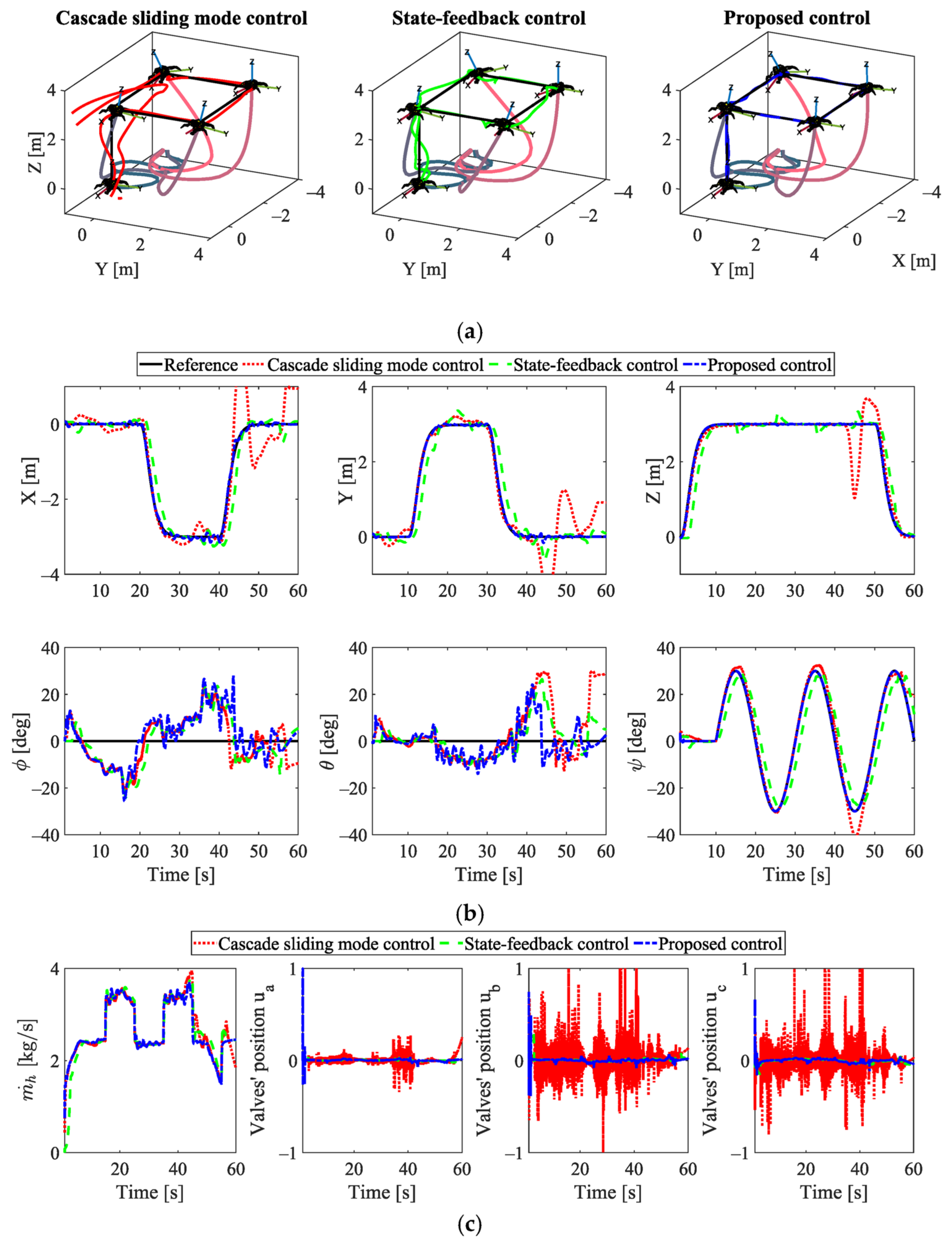
In this scenario, the system first takes off to a desired attitude of 3 [m] and maintains that height. It then tracks the desired setpoints in the corresponding horizontal plane and lands back on the ground at the end. Hence, the references of translational motions are in the form of step signals, and the setpoints are easily seen in Figure 5a. Moreover, a third-order filter was added for each signal to reflect the desired movements in practical operation. Thus, the resulting reference with respect to time is as in Figure 5b. During the process, the yaw angle of the head assembly also followed a sinusoidal trajectory, simulating the movement of widely spraying water to cover the flame. The resulting motions of the three control systems, including the head trajectory and postures of the head assembly and the hose, are shown in three-dimensional geometry in Figure 5a. The motion of the head assembly in every direction over time is given in Figure 5b. Moreover, their control inputs are subsequently illustrated in Figure 5c. In Figure 5d, every second, the posture of the hose is drawn once and then lined up side-by-side along the time axis. In this figure, the Y^*-axis represents the Y-coordinate being spread out with time. As shown, all the considered control systems can reach the required positions, but the two comparative ones exhibit several visible deviations from the reference. In detail, one can see that the cascade SMC system can track the references in real time. It gives a good tracking performance in the Z-direction, slight overshoot in the ψ-direction, and smooth transient responses in the horizontal translations. However, the controller must make allotted corrections in its control inputs, especially those for flow-regulating valves b and c as seen in Figure 5c. Even so, the resulting motions in the horizontal plane are poor. This is because the opening and closing of the valve lead to the fluctuation of the water flow and generate additional unwanted disturbance acting on the head assembly. As shown in Figure 5d, the more even distribution of the hose’s postures, the better its stability. In this sense, one can see the fluctuation of the hose due to this control action. On the other hand, the state-feedback control requires less control effort and provides smoother motions over time, but the motions tend to fall behind the desired trajectory. The horizontal motions are still not robust as their steady-state error can easily increase under the influence of other factors, although it is better than the results from the cascade SMC. For example, one can see in Figure 5b, between 20 [s] and 30 [s], while tracking the reference in the X-direction, that the cascade SMC and state-feedback controls cannot maintain their position in the Y-direction. Meanwhile, the proposed control system has good and real-time tracking performance in all directions during the whole simulation. The proposed system compensates effectively for the influence of couplings and disturbances so that the resulting translation and heading angles closely follow their corresponding references. It is also worth noting that due to the underactuated nature, the translations cannot be achieved without controlling the roll and pitch of the system. Hence, the proposed control system adjusts more in these two rotations compared to the comparative systems, but by doing so, it retains superior tracking performance in the horizontal plane. In terms of the control inputs, the proposed controller generates a large correction in the initial state, especially for the control signal of the valves. This is because of the low water flow rate in this state resulting in a small thrust force that requires the head assembly to lean more to correct its initial position and heading direction. After that, the adjustment of these inputs is still slightly larger than that of the state-feedback control (to achieve better motion performance) but significantly smaller than that of the cascade SMC. This results in better stability of the hose with the proposed control and the state-feedback control, in comparison to the cascade SMC.

In the second scenario of this reference type, the system’s performance was investigated in its application, i.e., the fire hose nozzle sprays water to perform firefighting actions. The obtained results are shown side-by-side in Figure 6a,d. The fire extinguishing flow has a rate of 1 [kg/s], being initiated at 15 [s], then lasting 10 [s] every 10 [s] interval. Not only does this flow generate an additional thrust acting on the head assembly, but it also changes the water supply leading to a fluctuation of the hose. The latter adds disturbances to the head and may even lead to flutter instability of the hose. The performance of the cascade SMC system is found to be unstable due to these disturbances. Meanwhile, the design of the two others takes the hose stability into account and hence preserves the stability of the whole system even though the fluctuation of the hose is still larger than in the first scenario, due to the change in the water supply for the firefighting action as mentioned. Moreover, the state-feedback controller can preserve the system stability but cannot reject disturbances effectively. Therefore, the resulting motions, especially the translations, are significantly affected. In contrast, the proposed control system retains good performance, with slight effects of disturbances visible in the X- and Y-directions.

5.3. Sinusoidal Trajectory Following

In this case, the head assembly is required to follow a continuous trajectory described by:

$$X_d=2\sin (0.15t),\hspace{0.17em}\hspace{0.17em}\hspace{0.17em}{Y}_d=3\sin (0.3t),\hspace{0.17em}\hspace{0.17em}\hspace{0.17em}{Z}_d=2+0.3\sin (0.2t)+0.03t$$

(45)

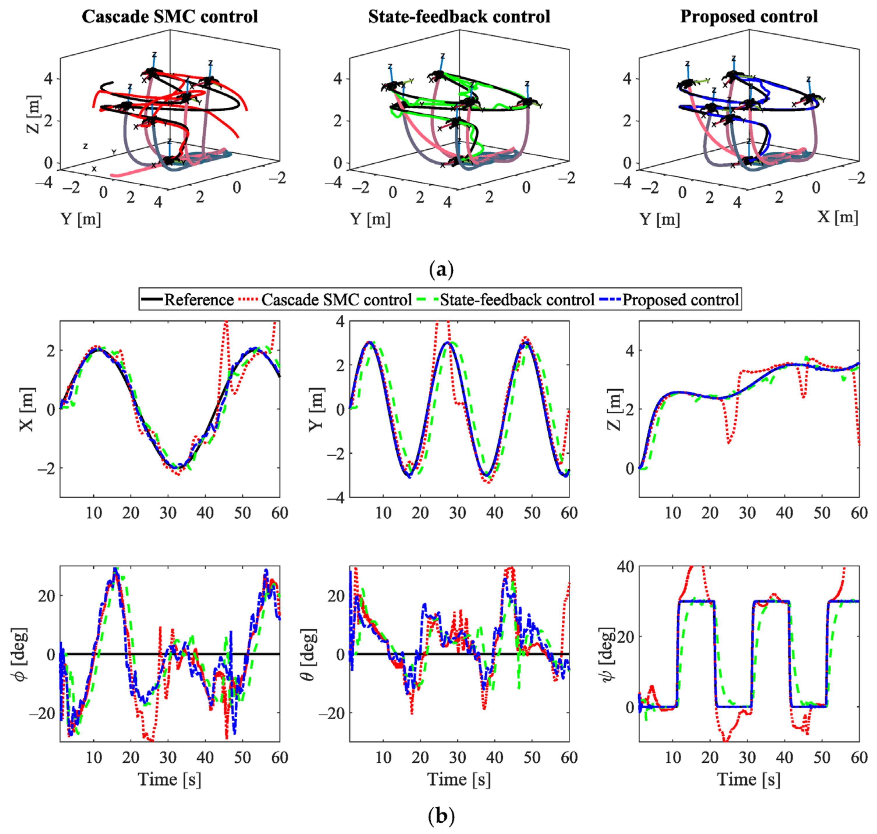
The required heading angle is in the form of a rectangular pulse signal, initialized at 11 [s], with an amplitude of $\pi /6$ [rad], lasting 10 [s] every 10 [s] interval. No fire extinguishing flow was considered in the first scenario with this reference. Figure 7a,d depict the simulation results in the same manner as the previous section. Similar results to those observed in the previous trajectory type can also be seen in this case. That is, the motions of the state-feedback control system fall behind the desired trajectories; the cascade SMC tracks the reference in real time but contains allotted deviation, and the proposed system remains the best solution. In the initial stage, all the control systems struggle to track their reference, due to the lack of water supply. Furthermore, all control systems experience challenges in tracking the translational motion smoothly, as the thrust force required to track the varying altitude changes. As seen in Equation (17), all acting torques are powered by this thrust. Hence, the flow-regulating valves must constantly adjust to retain the desired torques. In addition, the complex trajectory also leads to irregular shapes of the hose, such as twisting and releasing at around 45 [s] of the simulation. This obviously affects the motion of the head assembly and the stability of the hose, as visible in Figure 7a,b,d, and Supplementary Video S1. On the other note, the performance of the cascade SMC in the yaw motion is inferior to other controllers, despite being the second best controller in the previous reference. The cascade SMC quickly reaches the desired heading angle but cannot maintain a small steady-state error. In contrast, the state-feedback control system has a slow transient response but a small steady-state error. Meanwhile, the proposed system achieves excellent performance in the yaw direction, both transient and steady-state responses, as shown at the bottom right of Figure 7b.

In a similar intention to the second scenario with the step-type reference, the impact of firefighting actions was evaluated for this trajectory. The fire extinguishing flow was identical to the previous case, and its impact is visualized in the system performance in Figure 8. Accordingly, the cascade SMC is most affected followed by the state-feedback control and the proposed control that most effectively compensates for this firefighting action. Additionally, in

Table 3. Comparison of average performance indexes.

Control System	RMSE		ISV
	Position	Orientation	Flow Rate	Valve Operation
Cascade SMC control	0.328	0.141	425.725	0.505
State-feedback control	0.428	0.146	414.979	0.091
Proposed control	0.044	0.107	422.879	0.141

, two metrics are presented to evaluate the performance of the three control systems in the four simulations: the average root mean square errors (RMSEs) of the head motions and the integral of the square of the control input values (ISVs). The proposed control system shows superior positioning performance, as evidenced by a significant reduction in RMSE of 87% and 90% when compared to the cascade SMC and state-feedback control systems, respectively. However, for orientation, the average RMSE is not as good because the pitch and roll of the head must be alternated in order to position the system. When considering the yaw rotation only, the proposed system has a significantly better tracking performance, with an RMSE of 0.007 compared to 0.0162 and 0.124 in the cascade SMC and state-feedback systems, respectively. The ISV of the flow rate indicates that the proposed system consumes more water than the state-feedback control system but less than the SMC one. Fortunately, it is not a concern in water-based environments, which are the target application scenario of the proposed firefighting system. In the proposed system, the flow-regulating valves require more control actions than those with the state-feedback control but are significantly less intense than the cascade SMC system. From the results of the four simulation studies, the designed water-powered aerial system shows its capability, and the proposed control law demonstrates its superiority compared to the two control systems.

6. Conclusions

In this study, a novel water-powered aerial system with flow-regulating actuators and an effective control law was developed and validated. The system was inspired by hydroflight equipment and is capable of autonomous firefighting missions, particularly in or at bodies of water areas. The system comprises a water pump, a flexible hose, and a head assembly that can perform motions in three-dimensional space. The mathematical model was established to describe the dynamics of the whole system, and several dynamical characteristics were deduced from it. The proposed control law incorporates these characteristics into its design to result in the uniform ultimate boundedness of the system’s motion. Its effectiveness and robustness were evaluated via simulation studies, in which its motion performance and stability were compared to those controlled by different control approaches. Accordingly, the proposed system demonstrated its maneuverability and superiority. The system prototype will be fabricated, and experimental studies will be conducted for further evaluation.

References

- Robinson, B. Water Propelled Flying Board. U.S. Patent US9145206B1, 29 September 2015. [Google Scholar]
- Li, R. Personal Propulsion Device. U.S. Patent US7735772B2, 21 August 2007. [Google Scholar]
- Water—Zapata. Available online: https://www.zapata.com/en/water/ (accessed on 21 September 2022).
- Zapata, F. Maneuvering and Stability Control System for Jet-Pack. U.S. Patent US20140103165A1, 17 April 2014. [Google Scholar]
- Jetovator—Rise the Hose. Available online: https://www.jetovator.com/ (accessed on 21 September 2022).
- Qin, H.; Cui, J.Q.; Li, J.; Bi, Y.; Lan, M.; Shan, M.; Liu, W.; Wang, K.; Lin, F.; Zhang, Y.F.; et al. Design and implementation of an unmanned aerial vehicle for autonomous firefighting missions. In Proceedings of the 2016 12th IEEE International Conference on Control and Automation (ICCA), Kathmandu, Nepal, 1–3 June 2016; IEEE: Piscataway, NJ, USA, 2016; pp. 62–67. [Google Scholar]
- Spurny, V.; Pritzl, V.; Walter, V.; Petrlik, M.; Baca, T.; Stepan, P.; Zaitlik, D.; Saska, M. Autonomous Firefighting Inside Buildings by an Unmanned Aerial Vehicle. IEEE Access 2021, 9, 15872–15890. [Google Scholar] [CrossRef]
- EHang|Smart City Management—EHang 216F. Available online: https://www.ehang.com/ehang216f/ (accessed on 21 September 2022).
- High-Rise Firefighting with Dry Powder Fire Extinguishing—Guofei UAV. Available online: http://www.guofei-uav.com/index.php?c=article&a=type&tid=43 (accessed on 21 September 2022).
- Chaikalis, D.; Tzes, A.; Khorrami, F. Aerial Worker for Skyscraper Fire Fighting using a Water-Jetpack Inspired Approach. In Proceedings of the 2020 International Conference on Unmanned Aircraft Systems (ICUAS), Athens, Greece, 1–4 September 2020; pp. 1392–1397. [Google Scholar]
- Chaikalis, D.; Evangeliou, N.; Tzes, A.; Khorrami, F. Design, Modelling, Localization, and Control for Fire-Fighting Aerial Vehicles. In Proceedings of the 2022 30th Mediterranean Conference on Control and Automation (MED), Vouliagmeni, Greece, 28 June–1 July 2022; pp. 432–437. [Google Scholar]
- Lee, S.; Ng, W.; Liu, J.; Wong, S.; Srigrarom, S.; Foong, S. Flow-Induced Force Modeling and Active Compensation for a Fluid-Tethered Multirotor Aerial Craft during Pressurised Jetting. Drones 2022, 6, 88. [Google Scholar] [CrossRef]
- Viegas, C.; Chehreh, B.; Andrade, J.; Lourenço, J. Tethered UAV with Combined Multi-rotor and Water Jet Propulsion for Forest Fire Fighting. J. Intell. Robot. Syst. 2022, 104, 21. [Google Scholar] [CrossRef]
- Ausonio, E.; Bagnerini, P.; Ghio, M. Drone Swarms in Fire Suppression Activities: A Conceptual Framework. Drones 2021, 5, 17. [Google Scholar] [CrossRef]
- Harikumar, K.; Senthilnath, J.; Sundaram, S. Multi-UAV Oxyrrhis Marina-Inspired Search and Dynamic Formation Control for Forest Firefighting. IEEE Trans. Autom. Sci. Eng. 2019, 16, 863–873. [Google Scholar] [CrossRef]
- Dubai Firefighters Use Jetpacks to Aid High-Speed Response—Euronews. Available online: https://www.youtube.com/watch?v=H1VIxUTzb1I (accessed on 21 September 2022).
- Dubai Media Office. Available online: https://twitter.com/DXBMediaOffice/status/822797935176024065 (accessed on 20 February 2023).
- Ando, H.; Ambe, Y.; Ishii, A.; Konyo, M.; Tadakuma, K.; Maruyama, S.; Tadokoro, S. Aerial Hose Type Robot by Water Jet for Fire Fighting. IEEE Robot. Autom. Lett. 2018, 3, 1128–1135. [Google Scholar] [CrossRef]
- Ando, H.; Ambe, Y.; Yamaguchi, T.; Yamauchi, Y.; Konyo, M.; Tadakuma, K.; Maruyama, S.; Tadokoro, S. Fire extinguishment using a 4 m long flying-hose-type robot with multiple water-jet nozzles. Adv. Robot. 2020, 34, 700–714. [Google Scholar] [CrossRef]
- Ando, H.; Ambe, Y.; Yamaguchi, T.; Konyo, M.; Tadakuma, K.; Maruyama, S.; Tadokoro, S. Fire Fighting Tactics with Aerial Hose-type Robot “Dragon Firefighter”. In Proceedings of the 2019 IEEE International Conference on Advanced Robotics and its Social Impacts (ARSO), Beijing, China, 31 October–2 November 2019; IEEE: Piscataway, NJ, USA, 2019; pp. 291–297. [Google Scholar]
- Ando, H.; Ambe, Y.; Yamaguchi, T.; Konyo, M.; Tadakuma, K.; Maruyama, S.; Tadokoro, S. Activation of Hose by Multiple Water-Jet Injection Nozzles for Fire Fighting. Proc. JSME Annu. Conf. Robot. Mechatron. (Robomec) 2018, 2018, 2A1-M02. [Google Scholar] [CrossRef]
- Dinh, C.-T.; Huynh, T.; Kim, Y.-B. LQI Control System Design with GA Approach for Flying-Type Firefighting Robot Using Waterpower and Weight-Shifting Mechanism. Appl. Sci. 2022, 12, 9334. [Google Scholar] [CrossRef]
- Liu, X.; Zhou, H. Unmanned Water-Powered Aerial Vehicles: Theory and Experiments. IEEE Access 2019, 7, 15349–15356. [Google Scholar] [CrossRef]
- Ambe, Y.; Yamauchi, Y.; Konyo, M.; Tadakuma, K.; Tadokoro, S. Stabilized Controller for Jet Actuated Cantilevered Pipe Using Damping Effect of an Internal Flowing Fluid. IEEE Access 2022, 10, 5238–5249. [Google Scholar] [CrossRef]
- Yamaguchi, T.; Ambe, Y.; Ando, H.; Konyo, M.; Tadakuma, K.; Maruyama, S.; Tadokoro, S. A Mechanical Approach to Suppress the Oscillation of a Long Continuum Robot Flying With Water Jets. IEEE Robot. Autom. Lett. 2019, 4, 4346–4353. [Google Scholar] [CrossRef]
- Ambe, Y.; Ando, H.; Konyo, M.; Tadokoro, S. Design of a simple controller for the flying hose type robot with water jet. In The Proceedings of JSME annual Conference on Robotics and Mechatronics (Robomec), Fukushima, Japan, 10 – 13 May 2017; The Japan Society of Mechanical Engineers: Shinjuku-ku, Tokyo, Japan, 2017; p. 1P1-P02. [Google Scholar]
- Yamauchi, Y.; Ambe, Y.; Konyo, M.; Tadakuma, K.; Tadokoro, S. Realizing Large Shape Deformations of a Flying Continuum Robot with a Passive Rotating Nozzle Unit That Enlarges Jet Directions in Three-Dimensional Space. IEEE Access 2022, 10, 37646–37657. [Google Scholar] [CrossRef]
- Yamauchi, Y.; Ambe, Y.; Konyo, M.; Tadakuma, K.; Tadokoro, S. Passive Orientation Control of Nozzle Unit with Multiple Water Jets to Expand the Net Force Direction Range for Aerial Hose-Type Robots. IEEE Robot. Autom. Lett. 2021, 6, 5634–5641. [Google Scholar] [CrossRef]
- Lee, D.-H.; Huynh, T.; Kim, Y.-B.; Soumayya, C. Motion Control System Design for a Flying-Type Firefighting System with Water Jet Actuators. Actuators 2021, 10, 275. [Google Scholar] [CrossRef]
- Samadikhoshkho, Z.; Lipsett, M. Decoupled Control Design of Aerial Manipulation Systems for Vegetation Sampling Application. Drones 2023, 7, 110. [Google Scholar] [CrossRef]
- Shi, C.; Wang, K.; Yu, Y. Expandable Fully Actuated Aerial Vehicle Assembly: Geometric Control Adapted from an Existing Flight Controller and Real-World Prototype Implementation. Drones 2022, 6, 272. [Google Scholar] [CrossRef]
- Yu, Y.; Shi, C.; Shan, D.; Lippiello, V.; Yang, Y. A hierarchical control scheme for multiple aerial vehicle transportation systems with uncertainties and state/input constraints. Appl. Math. Model. 2022, 109, 651–678. [Google Scholar] [CrossRef]
- Chen, W.; Dai, H.; Wang, L. Three-dimensional dynamical model for cantilevered pipes conveying fluid under large deformation. J. Fluids Struct. 2021, 105, 103329. [Google Scholar] [CrossRef]
- Wadham-Gagnon, M.; Paı¨doussis, M.P.; Semler, C. Dynamics of cantilevered pipes conveying fluid. Part 1: Nonlinear equations of three-dimensional motion. J. Fluids Struct. 2007, 23, 545–567. [Google Scholar] [CrossRef]
- Paidoussis, M.P. Fluid-Structure Interactions: Slender Structures and Axial Flow; Academic Press: Cambridge, MA, USA, 1998; Volume 1, ISBN 008053175X. [Google Scholar]
- He, W.; He, X.; Ge, S.S. Vibration Control of Flexible Marine Riser Systems with Input Saturation. IEEE/ASME Trans. Mechatron. 2016, 21, 254–265. [Google Scholar] [CrossRef]
- He, W.; Zhang, S.; Ge, S.S. Boundary Control of a Flexible Riser With the Application to Marine Installation. IEEE Trans. Ind. Electron. 2013, 60, 5802–5810. [Google Scholar] [CrossRef]
- He, W.; He, X.; Sam Ge, S. Modeling and Vibration Control of a Coupled Vessel-Mooring-Riser System. IEEE/ASME Trans. Mechatron. 2015, 20, 2832–2840. [Google Scholar] [CrossRef]
- He, W.; Sun, C.; Ge, S.S. Top tension control of a flexible marine riser by using integral-barrier lyapunov function. IEEE/ASME Trans. Mechatron. 2015, 20, 497–505. [Google Scholar] [CrossRef]
- Ge, S.S.; He, W.; How, B.V.E.; Choo, Y.S. Boundary Control of a Coupled Nonlinear Flexible Marine Riser. IEEE Trans. Control. Syst. Technol. 2010, 18, 1080–1091. [Google Scholar] [CrossRef]
- Huynh, T.; Lee, D.-H.; Kim, Y.-B. Study on Actuator Performance Evaluation of Aerial Water-powered System for Firefighting Applications. Appl. Sci. 2023, 13, 1965. [Google Scholar] [CrossRef]
- Li, R. Personal propulsion devices with improved balance. U.S. Patent US9849980B2, 18 September 2014. [Google Scholar]
- Sahoo, P.K. Some results related to the integral mean value theorem. Int. J. Math. Educ. Sci. Technol. 2007, 38, 818–822. [Google Scholar] [CrossRef]
- Leader, J.J. Numerical Analysis and Scientific Computation; CRC Press: Boca Raton, FL, USA, 2022; ISBN 1000540391. [Google Scholar]
Figure 1.
Putting out a boat fire.
Figure 2.
The proposed aerial water-powered firefighting system with flow rate control: (a) Proposed system concept drawing and (b) Diagram of water flow in the head part.
Figure 3.
Coordinate definition and forces analysis.
Figure 4.
Structure of the proposed control system.
Figure 5.
Motion performance in the case of step-type reference tracking. (a) Tracking performance in 3-dimensional geometry; (b) Time responses of translations and rotations; (c) Three-dimensional partial motion of the water-conveying hose; and (d) Control inputs.
Figure 6.
Motion performance in the case of step-type reference tracking with firefighting action. (a) Tracking performance in 3-dimensional geometry; (b) Time responses of translations and rotations; (c) Three-dimensional partial motion of the water-conveying hose; and (d) Control inputs.
Figure 7.
Motion performance in the case of sinusoidal trajectory following. (a) Tracking performance in 3-dimensional geometry; (b) Time responses of translations and rotations; (c) Three-dimensional partial motion of the water-conveying hose; and (d) Control inputs.
Figure 8.